Light harvesting improvement of organic solar cells with ...

Characterization and improvement of a direct solar radiation detector
By
Marcelino Adriano Macome
BSc (Hons)
A thesis submitted in fulfillment of the requirements for the degree
of Master of Science in Physics in the Faculty of Science at the
University of KwaZulu-Natal (Westville campus)
Supervisor: Prof. M. McPherson
December 2004

Declaration
The Registrar (Academic)
University of KwaZulu-Natal (Westville)
Dear Madam
I, Marcelino Adriaro Macome
Reg.: 200300066
Degree: MSc Physics
Hereby declare t^at the dissertation entitled "Characterization and
improvement of a direct solar radiation detector" is the result of my own
investigation and research and that it has not been submitted in part or in full
for any other degree or to any other University.
December 13 ,2004
Signature
4gggL;
ii

Dedication
This thesis is dedicated with love and gratitude to the memory of my elder brother, to my
father Marcelino and to my sister Virginia.
iii

Acknowledgements
Many people have contributed to make this dissertation a reality. My gratefulness goes to
all staff of the Department of Physics of the University of KwaZulu-Natal (Westville
Campus). I wish to thank amongst them Mr. R. van den Heetkamp for his support,
fruitful advice from the very start and most importantly for his friendly attitude. I also
acknowledge with thaiiks Mr. F. Hoffman of the Academic Instrumentation Unity for his
technical support and advice in the construction of the detector.
More especially, I appreciate the constructive supervision and patient guidance from my
supervisor Prof. M. McPherson. I have also to thank my colleagues for stimulating
discussions and advice, especially Mr. E. Zhandire and Mr. A. Mawire. I would like to
extend my thanks to my family for their love and encouragement. I also wish to thank
Clementina whose love, support and encouragement have always been there.
Finally I wish to thank the University of Eduardo Mondlane in Mozambique through the
Renewable Energy program for financing my studies and my stay in Durban. I also thank
Dr. M. Chenene and Dr. G. Mahumane for their readily available advice, and more
especially Dr. B. Cuamba for his very useful assistance.
IV

Abstract
A low-cost Direct Solar Radiation Detector (DSRD) was developed in house in the
Department of Physics at the University of KwaZulu-Natal (Westville). A main use of
this instrument is to gather solar energy data that are to be used in the design of systems
that concentrate and convert solar energy into thermal energy (concentrating solar
thermal energy systems). These data are compiled into a database from which the
efficiency and potential use of many solar systems can be based.
It was required that the detector was fully characterized with respect to spectral range,
polar (angular) response and environmental stability. Based on this analysis it was also
required to investigate possible ways of improving the detector. An Eppley Normal
Incidence Pyrheliometer (NIP) mounted on an Eppley Sun Tracker (ST) was used as a
reference instrument. The ST is a power driven tracker with an axis parallel to the Earth's
axis of rotation. The NIP and DSRD were mounted together on the tracker in order to
correlate their responses and also to calibrate the DSRD.
The results indicate that the modified DSRD works better in that it follows the reference
instrument. The correlation between the NIP data and the DSRD data is better with the
value of correlation factor close to unity and the root mean square error value close to
zero. This means that the modifications carried out on the detector have improved the low
cost in-house detector and hence the quality of data collected.
• " . ; „ , • $ •

Chapter 1
For any scientific discipline to remain active and productive effectively and efficiently,
the power of its instrumentation must grow significantly with time. Without this growth
the discipline tends to stagnate and no new discoveries are made. This means that for the
field of Science and Technology the development of instrumentation is paramount. As
time passes, high-level functionality and simplicity for low cost instrumentation is needed
depending on the complexity of the application needs.
An accurate assessment of solar resources is based upon accurately measured data. In
particular, data on the spatial distribution of measured solar radiation, especially over a
period of time, can be used in models as the basis for many engineering designs and
economic decisions.
In most countries, a reliable and sustainable energy supply is very crucial in the context
of economic development and may often be used as a measure against poverty. Statistics
show that major parts of suburban and rural Africa, and many areas in the world, are
1
v'^..

located in non-electrified areas [Gore, 2003]. The population in these areas depends on
expensive and inconvenient energy sources like wood, coal, petroleum, paraffin, batteries
and candles. These are also the most polluting sources of energy. A large number of
schools are located in the areas with no electricity, thereby going to enormous problems
to get water pumped and well treated. A lack of good treatment of water leads to a high
possibility for diseases carried by contaminated water.
Solar radiation is a guaranteed and cheap infinite source of energy to any community in
any part of the world. This is especially true for the rural areas in the countries situated
inside the Sunbelt (that is 40° north to 40° south) [Cuamba et al, 2001]. Solar energy does
not need a grid connection as compared to other sources of energy, in particular, the
nonrenewable fuels. It is thus always close to where it is needed and does not cause any
negative impacts to the environment.
Solar radiation is the main energy input that determines the physical, chemical and
biological dynamics of landscape processes with a direct impact on human living. An
understanding of solar radiation in terms of its properties and availability is a logical start
to the discussion of its practical application as a source of energy. A means to capture
solar radiation and to convert it into a useful energy resource is of paramount importance.
An interpretation of solar radiation data in determining the influence of solar radiation
over innumerable natural dynamic processes such as natural catastrophes, climatic
changes and biological effects is also very important.
2

1.1 Aims and objectives
A main aim of the project is the characterization and improvement of an in-house Direct
Solar Radiation Detector (DSRD). The improvement on the detector is expected to ensure
that good quality and reliable data are collected. Thus, an indirect objective of the project
is to improve the quality and reliability of collected solar radiation data.
1.2 Solar radia t ion spec t rum
The electromagnetic spectrum extends from a wavelength of 10 to 10" m [McDaniels,
1984]. A concern of this research work is only a very small part of this spectrum, the
solar radiation spectrum or SRS, which extends from a wavelength of-300 nm to -3000
nm. The SRS is made up of three main regions; the ultraviolet (UV) region, the visible
region and the infrared (IR) region [Twidell and Weir, 1996].
1.2.1 The UV region
The ultraviolet or UV region of the SRS corresponds to wavelengths less than -380 nm
[Duffie and Beckman, 1991]. Ultraviolet radiation can not be detected by the human eye.
A large amount of UV radiation is absorbed by atmospheric contents before it reaches the
earth's surface. The smallest part of solar energy that reaches the surface of the earth is
UV radiation.
3

1.2.2 The visible region
The visible region of the SRS is a part of the solar radiation spectrum that can be detected
by the human eye and covers a wavelength from -380 to -780 nm [Duffie and Beckman,
1991]. The atmosphere is almost completely transparent to solar radiation in the visible
region [Twidell and Weir, 1996]. Therefore, the largest part of solar energy that reaches
the earth's surface is in the visible region.
1.2.3 The infrared region
The infrared or IR region of the SRS comprises all radiation with wavelengths greater
than -780 nm [Duffie and Beckman, 1991]. Infrared radiation is emitted by all objects
that are at any temperature below -700 K [Mcdaniels, 1984]. Water vapor and carbon
dioxide in the atmosphere absorb about 20 % of the radiation in the IR region [Twidell
and Weir, 1996], and so only about 80 % of this radiation reaches the surface of the earth.
1.3 Characterization methods
The characterization of the DSRD has been carried out with respect to its spectral
response, its polar response and its environmental stability.
1.3.1 Spectral response
The characterization of the DSRD with respect to spectral response is a detailed account
of how the detector responds to different wavelengths of solar radiation. It is a
4

requirement that the detector responds evenly to the same amount of energy and this
response must be independent of the wavelength of the solar radiation.
1.3.2 Polar response
The characterization of the DSRD with respect to polar response is an account of the
behaviour of the detector when it is misaligned with respect to the normal incidence of
the radiation beam. If the collimating hole in front of the detector is not at a slope equal
to that of the NIP, various errors may be introduced in the readings especially by
reflection from the sides of the hole such that the DSRD overheads.
1.3.3 Environmental stability
By virtue of it being a detector of solar radiation, the DSRD is placed out doors where it
is subjected to certain atmospheric elements that may damage or distort the readings of
the detector. It is desirable, therefore, that the detector is tolerant to the instability of
environmental effects such as rain, humidity, wind and any adverse temperature changes.
1.4 Perceived improvement
Based on the preceding statements, it is perceived that an improvement of the DSRD will
be based on its spectral response to direct solar radiation, on its polar response to this
radiation and on its physical location.
5

1.4.1 Spectral response
The curve of the spectral responsivity of the DSRD indicates that even though the
detector is a direct solar radiation detector, it is sensitive to IR radiation as well. Thus, it
is highly likely that the detector reads direct as well as diffused radiations. Several optical
glass filters will be investigated to minimize the detection of other radiations besides
direct solar radiation.
1.4.2 Polar response
When light strikes any surface, it may undergo all the known optical effects. For the
DSRD these effects will be maximum when the collimating hole is not properly aligned
with the direction of the sunlight. This may cause detections of unwanted components of
the incident solar radiation. The viewing angle of the detector must be aligned properly
for the collimating hole to coincide with the direction of the sunlight.
1.4.3 Environmental stability
The housing of the DSRD is not very well sealed such that it allows moisture to
accumulate onto the detector surface. The collimating hole is open to the atmosphere and
so allows moisture an<1 rain to accumulate onto the detecting surface and this will affect
the readings. The black colour of the housing absorbs radiation and this may have the
effect of raising the temperature of the interior of the housing which may affect the
detecting surface. An increase in temperature is known to increase the measured current
6

[McPherson, 2004a] in diodes of this type. An improvement to the DSRD would involve
proper sealing and possibly the use of a white housing.
1.5 Brief description of the DSRD
The DSRD is made up of an integrated circuit (IC) and an external circuit (EC) both of
which are housed in a rectangular plastic box with holes for feeding electrical signals to a
data logger and for collimating the solar beam.
The IC is an OPT101 monolithic circuit which consists mainly of a photodiode and an
amplifier. The photodiode is operated in the photoconductive mode, it has an active area
of 5.244 mm2. It detects radiation in the wavelength range of-280 to ~1100 nm and it is
connected such that the incident radiation is converted into a current. Its spectral response
varies with respect to the wavelength and it peaks at 850 nm [Burr-Brown, 1996]. The
amplifier is connected such that it converts current generated from the photodiode into an
output voltage which increases linearly with the intensity of solar radiation. This
amplifier is able to handle both single and dual power supplies and is therefore ideal for
battery operated equipment like the DSRD.
The EC circuit is made up of a variable resistor and a battery. The variable resistor is
connected in series with the internal resistor of the amplifier in the IC, and this helps to
increase the responsivity of the amplifier. The battery is used mainly for supplying power
7

to the whole circuit. However, the battery is also used for its low noise output such that
the overall electrical noise of the system is minimal [McPherson, 2003].
1.6 Thesis outline
The thesis consists of five chapters, beginning with this introduction. Chapter 2 outlines
the theory that served as background to this present project and consists mainly of a
description of the interaction between solar radiation and the earth. In particular, a brief
description of the concepts evolving in interaction between the sun, the earth and the
atmosphere.
Chapter 3 is a description of the experimental procedure carried out. The experiment
concentrates on measuring direct solar radiation using the DSRD to be improved. The
readings from the DSRD are then compared with those of the reference instrument to
establish the improvement required. Afterwards, several measurements were carried out
to test the DSRD and to establish how the improvements could be incorporated. A
description of the data acquisition system and the calibration technique are also included
in this chapter.
Chapter 4 is a presentation and a discussion of the results, the analysis of which have
established that the improvements on the DSRD have improved the quality of data taken.
In this way, they show that the characterization was necessary. The thesis ends with
8

chapter 5 which is uV conclusion based on the results. Here possible future work for
further improvement of the DSRD is also presented.
l)

Chapter 2
Theory
Solar radiation is a form of electromagnetic energy emitted by the sun and it travels
through space in the form of a wave. There are various reasons for studying solar
radiation. Often solar radiation is studied for climatological, synoptic, biological or
energetic purposes. The spectral distribution of solar radiation is worthy of study since
the absorption, transmission and reflection of radiation by any object is dependent upon
the wavelength of the radiation as well as the type of absorbent material, the properties of
the absorbing surface and the angle of incidence [Twidell and Weir, 1996].
2.1 Solar Radiation Spectrum
Solar radiation incident onto the top of the earth's atmosphere can be classified into three
main regions with respect to the wavelength, and this is called the solar radiation
spectrum or SRS. Figure 2.1 shows the spectral distribution of solar radiation and this
10

represents the compiled standard spectrum based on high altitude and space
measurements [Twidell and Weir, 1996].
xlO T-
a a
S
1 -
0 1 • • ' •• • • ^ • • fc • ' ' • '
300 1000 2000
Wavelength (nm)
3000
Figure 2.1: A curve of the standard spectral extraterrestrial irradiance at mean earth-sun distance adopted by the World Radiation Center (WRC) [after Twidell and Weir, 1996]. The area under the curve represents the amount of solar energy available at the top of the atmosphere.
The first region of the SRS is made up of short wavelength radiation, commonly known
as ultraviolet (UV) radiation. The UV itself is divided into three regions. The first region
extends up to 280 nm, the second between 280 and 350 nm and the third covers the range
between 350 and 380 nm. The atmosphere serves as a filter by preventing UV radiation
from reaching the earth's surface. The first part of UV radiation is completely blocked by
atmospheric gases like oxygen (O2) and ozone (O3). This first part is also radiation that is
*
11

biologically harmful. The second and third parts of UV radiation are able to reach the
earth's surface even though they are severely scattered by atmospheric gases. UV
radiation has a practical use in water disinfection [Twidell and Weir, 1996] because of its
high potential to penetrate matter.
The second region of the SRS is made up of radiation of medium wavelengths and is
called the visible spectrum since it can be perceived by the human eye. The visible
spectrum is an extremely narrow band when compared to the other bands. Nevertheless,
about half of the solar energy incident at sea level is in this region which extends from
-380 to -780 nm [Duffie and Beckman, 1991]. A clear sky becomes an open window for
visible solar radiation to reach the earth's surface. For this reason, the amount of solar
energy measured at sea level is significantly in the visible band of the SRS.
The third and last region of the SRS extends to all wavelengths greater than -780 nm
[Duffie and Beckman, 1991] and is commonly called the infrared (IR) region. Because of
the long wavelengths, it is the most highly reflected radiation of the spectrum. IR
radiation can be emitted by any object at temperatures lower than -700 K. [McDaniels,
1984], even at ambient temperature. IR radiation represents almost 50 % of
extraterrestrial solar radiation and -20 % of this is absorbed by water vapor and carbon
dioxide present in the atmosphere. This IR radiation represents a small fraction of energy
emitted by the sun and measured at sea level.
12

Approximately 99 % of solar energy reaching the earth's surface is contained in the
region between 300 and 3000 nm. The distribution of solar energy as shown by the SRS
indicates that 9 % of solar energy reaching the earth's surface is in the UV region, 49 %
is in the visible spectrum and 42 % is in the IR region. This is based on an air mass ratio
equal to 1 [McDaniels, 1984]. This absorption at different wavelengths is shown in the
spectrum of Figure 2.2.
30C 1000 2000 3000
Wavelength (nm)
Figure 2.2: The SRS based on the solar radiation measured at sea level [after Website 2], This spectrum reveals the attenuation of solar radiation by the atmosphere. The shaded area indicates the radiation that does not reach the earth.
13

2.2 Attenuating effect of the earth's atmosphere
The solar radiation that reaches the top of the terrestrial atmosphere is referred to as
extraterrestrial radiation. The estimated amount of this radiation per unit time, per unit
area (of a surface perpendicular to the direction of propagation), at mean sun-earth
distance, is 1367 Wm". This figure has been adopted by the World Radiation Center
(WRC) and is called the solar constant [Duffie and Beckman, 1991]. Nevertheless,
almost half of this radiation is absorbed by air molecules or reflected and scattered by
clouds and small atmospheric particles before it reaches the earth's surface.
The absorption and scattering levels of the atmosphere depend on the amount of air mass
between the observer and the sun. This means that the absorption and scattering
mechanisms are functions of the number of particles that the radiation must pass through.
Solar radiation scattering is also a function of the size of particles relative to the
wavelength of the radiation [Website 2]. The air mass is basically comprised of water
vapor, gases and solid particles that are present in the atmosphere.
The path length of solar radiation towards the earth's surface through air molecules
changes with time and this will be discussed in Section 2.3. The lower the sun is in the
sky with respect to a detector (or to an Observer) on the earth's surface (that is around
sunrise or sunset) the longer the path length between the sun and the earth's surface. It is
also valid to say that in this situation, the air mass between the sun and the earth is
greater. The minimum amount of air mass occurs at solar noon in any given clear day.
14

The attenuation of solar radiation by gas constituents in the atmosphere describes clear
and dry conditions and is given by the optical air mass and the optical thickness. The blue
color of the clear sky is a result of blue light scattering by air molecules in the third
region of the UV spectrum. When the sun rises or sets, the path of the solar beam is
longer with the result that the blue light scattering is more pronounced such that red light
is dominant. The oveiall result is that the sky appears red [Website 2].
Clouds are the strongest attenuators of solar radiation. This attenuation depends on the
optical properties of the clouds, the position and number of layers of clouds through the
atmosphere, as well as the thickness and density of the clouds [Website 4]. The most
significant process in cloud attenuation is reflection. Very dense clouds, about a km in
thickness, are said to reflect back into space 90 % of the incident solar radiation [Website
1]. Figure 2.3 is a diagram that summarises the different attenuation aspects of solar
radiation.
In many applications, a study of solar radiation under clear sky conditions is very
important. Maximum solar energy is obtained when the sky is clear and dry. Terrain
topography like inclinations, as well as shadowing effects of neighboring terrain features,
modify the radiation input to the earth's surface in different locations. The elevation
above sea level determines the attenuation of radiation by the thickness of the atmosphere
[Website 4].
15

Figure 2.3: A diagram that shows the attenuation of solar radiation by atmospheric components and the significant attenuating process for each atmospheric constituent [after McDaniels, 1984].
2.3 Sun-Earth geometry
A measurement of direct solar radiation requires a sun tracking system for continuous
readings. The position of the sun in the sky for a given latitude, longitude, year, day and
time can be determined from the geometry of the sun-earth system and is very important
for a good orientation of the collector surfaces.
16

To an observer on the earth the sun apparently moves across the sky following a circular
arc from horizon to horizon [Website 3]. Figure 2.4 is a schematic representation of the
path of the sun across the sky and of the incident beam through atmosphere towards the
surface of the earth for a given day. The basic parameters for the determination of the
sun's position for a particular time are also indicated.
Figure 2.4 shows that the strength of the incident solar beam for any horizontal surface
depends on the position of the sun in the sky and this is defined by a zenith angle, 6. The
greater the value of 6, the weaker the incident solar radiation and this means that the path
length of the incident solar radiation is larger for a large value of 8. The opposite is also
true.
Incident
beam
*
Normal to horizontal
N
Horizontal surface
Figure 2.4: A diagram that shows the sun's path as seen by an observer on the earth's surface for a given day. The sun's position can be described in terms of the zenith angle (6), the azimuth angle 0?) and the solar altitude angle (ft).
17

The declination (S) is the angular position of the sun at solar noon with respect to the
plane of the equator [Duffie and Beckman, 1991]. In other words, it is the latitude of the
point where the sun is overhead at solar noon, south negative. It varies from -23.45° to
23.45° throughout the year according to the variation of the seasons. The declination
expresses the tilt of the axis of the earth rotation relative to the sun for a given day.
Figure 2.5 illustrates the variation of the declination with respect to the earth's plane of
rotation for particular days during the year. It is of interest to mention that the declination
varies smoothly from a positive number at midwinter to a negative number at midsummer
for the southern hemisphere.
March 20-22 Jwae 21-22 Septembei 22-2:1 December 21-22
Figure 2.5: The earth as seen from a point far from its orbit and the variation of the declination for particular days of the year for the southern hemisphere [after Twidell and Weir, 1996]. In June, the north pole is inclined near to the sun and so has more sunshine, while in December the same is true for the south pole.
Several definitions based on empirical approximations are presented in the literature for
the declmation. One of them is [Duffie and Beckman, 1991]
18

5 = 23.45sin (284+ «) 365
(2.1)
where 23.45 is the maximum value of the sun's declination (d0) when the sun is exactly
above one of the tropics and this corresponds to December 21-22 and June 21-22 (see
Fig. 2.5). The value of 360 is the maximum angle of revolution of the earth around the
sun in a 365 day-long year and n is the day number in a year where on 1 January n = 1
and on 31st December n = 365 (or 366 in a leap year). The value of n for any day of the
month can be found by use of Table 2.1. Here, the value of 284 is an empirical value
suggested by Duffie and Beckman [1991].
Table 2.1: The number of days in a year (n) for the j day of the month [after Duffie and Beckman, 1991]
Month n for j* day of Date month (j)
n day of year
January February March April May June July August September October November December
j
31+j 59+j 90+j 120+j 151+j 181+j 212+j 243+j 273+j 304+j 334+j
10 20 2 15 11 17 25 30 10 21 18 31
10 51 61 105 131 168 206 242 253 294 322 365
St 1 Note: In a leap year February has 29 days in this case on 3ls December n = 366.
The solar altitude (ft) is the angle in a vertical plane between the sun's rays and the
projection of the sun's rays on the horizontal plane, while the latitude (<p) is the engular
location of a given point on the earth's surface south or north of the equator and it is
19

considered positive in the north. It varies between -90° at the South Pole and 90° at the
North Pole.
The azimuth angle (y/) is the angular displacement of the projection of beam radiation
on the horizontal surface, measured from the south. Conventionally, in the southern
hemisphere, y is negative for surfaces that face east of north and positive for surfaces
that face west of north [Duffie and Beckman, 1991]. The hourly angle (ay) represents the
angular displacement of the sun. This is measured east or west of the local meridian due
to the earth's rotation around its axis at one degree per four minutes. The hourly angle is
negative in the morning and positive in the afternoon.
The zenith angle (&) is the angle between the sun's rays and the local vertical. This is the
angle of incidence of beam radiation with respect to an imaginary line perpendicular to a
horizontal surface at the site in question. The zenith angle changes from 0° when the solar
beam is perpendicula- to the horizontal surface, to 90° when the sun is at the lowest point
in the sky. For a horizontal surface, the zenith angle is defined analytically as
cos 0 = cos <p cos S cos & + sin (p sin 5 (2.2)
where q> ii she eocal latitudee 6 ii she eun's declinatton and c is the eourly yngle. The
angle of incidence (9^) is the angle between the line of incident solar radiation onto a
surface and the normal to that surface. If the surface is placed horizontally, # — #0.
Maximum solar radiation collection occurs when the surface of a solar collector is placed
such that the angle of incidence is equal to zero and this is when the solar beam is normal
to the surface.
20

Although, the earth's orbit is assumed to be circular in most cases, it is actually elliptical.
Therefore, the distance between the sun and the earth changes as the earth makes its
passage around the sun throughout the year and this causes the seasons. The earth's daily
rotation around its axis and its yearly revolution around the sun both contribute
significantly to the variation and distribution of solar radiation over its surface. Figure 2.6
illustrates the orbit of the earth and the variations in the distance between sun and earth
during the earth's revolution around the sun.
June 21-22 Winter solstice
N March 20-22 Spring equinox
Sept. 22-23 § Autumn equinox
S Dec. 21-22 Summer solstice
Figure 2.6: The orbit of the earth around the sun showing the solstice and equinoxes, as well as the changes in the sun-earth distance during the earth's revolution
The daily rotation of the earth around its axis and the interaction between sun's rays and
the earth's surface is shown in Fig. 2.7.
21

66 55*
S U M ' s
Ri"Ts
S^S"
I PlFUtC (J f UJ'bit
Figure 2.7: J representation of the sun 's rays as they interact with the earth 's surface [after Website 3J. As the earth rotates, the points located in the shaded part move towards the illuminated vart of the earth.
In addition to this, the changing length of daylight and darkness as well as the changing
of seasons has to be taken into account in any calculations and designs.
When the sun sets, the zenith angle 9 = 90° and by Eq. (2.2), the sunset angle will be
given by
costa, =-tan<ptanS (2-3)
where &>s is the sunset angle, which is just the angular displacement of the sun as
measured with respect to solar noon. The length of day is a function of declination and
latitude. Since Eq. (2.3) gives the length of the day from midday it is multiplied by 2 to
obtain the length of day N, hence
N = —cos 1 ( - tanq tan £ I 1 5
(2.4)
22

where 15 (=360°-r24 hours) is used to convert the result in Eq. (2.4) from degrees to
hours since the earth covers 360° in 24 hours, S is the angle of the sun's declination and
(p ii she latitude of fhe eocation.
2.4 Solar t ime (ST) and local clock t ime (LCT)
Solar time is a basic parameter used in solar radiation calculations and does not coincide
with local clock time [Duffie and Beckman, 1991]. A clock day is exactly 24 hours while
a solar day differs slightly at -24.25 hours [Website 3]. This is because the earth's
rotation and the obliquity of the earth's orbit are not regular. The earth, during its rotation
and revolution, is subjected to gravitational interactions with other planets in the solar
system. These interactions are one of the sources of the differences in time. In scientific
or engineering calculations it is necessary to convert clock time to solar time for better
accuracy.
The equation of time gives the difference between solar time and local clock time. It is
given by [Website 3]
£ = 0.165 sin 25 -0.126 cos B -0.025 sin B (2.5)
in hours, where B is a day angle in degrees and is given by
g = ' ' (2.6) 365
•
where 360 is as defined inEq. (2.1) for a 365 day year and n is the day number in a year.
The relationship between solar time (ST) and local clock time (LCT) is given by
23

ST = LCT + — (£,„d +Lj/U.)+E (2.7) 15
where 15 is as defined in Eq. (2.4). Here Lsttf is the longitude of the Standard Meridian
for the local time zone and L\oc is the longitude of actual location both in degrees west
and degrees east according to localization of the observer in relation to Greenwich
Meridian.
Once solar time is established, the hour angle co can nb ealculated. By yoting that the
hour angle varies at the rate of 15° per hour, that a> = 0 at solar noon and that the sign
convention is a < 0 0bfore sslar roon, ,he equation for hour rngll ei
co = \1{ST —12) (2.8)
where 12 is the number of hours elapsed from solar midnight to noon.
2.5 Spatial distribution of solar radiation
Solar radiation is unevenly distributed [Website 1], varies in intensity from one
geographic location to another and depends on the latitude, longitude, elevation, season
and time of day. A large area of die southern hemisphere is occupied by the oceans and
this factor contributes strongly to the amount of cloud cover. This is one source of the
difference between the southern and northern hemispheres in terms of the availability of
solar radiation.
24

The geographic distribution of total solar radiation on a global scale is divided according
to its intensity into four broad belts around the earth [Website 1]. Figure 2.8 illustrates the
geographic distribution of solar radiation. This distribution is very important for the
• Best conditions Good conditions Fair conditions Poor conditions
Figure 2.8: A worldwide distribution of solar radiation into belts indicating the feasibility of solar applications [after Website 1] around the globe.
assessment of the feasibility of solar applications in different locations around the globe.
2.5.1 The belt with the best conditions of sunshine.
The best conditions belt corresponds to regions situated between latitudes 15° and 35°
south (or north) of the equator. These regions are climatically semi-arid and so they
receive large amounts of direct solar radiation, mainly because of limited cloud coverage
25

and rainfall throughout the year. It is estimated that 3000 hours of sunshine per year are
available [Website 1] ]n this belt.
2.5.2 The belt with good conditions of sunshine
The regions of good conditions of sunshine comprise the region between latitudes 15°
south and 15° north of the equator. Unlike the belt with the best conditions, the cloud
cover here is most frequent, with the consequence that the precipitation level is high.
Associated with a high frequency of precipitation is high humidity with the consequence
that there is a high proportion of scattering and reflection of solar radiation. The average
number of sunshine hours is estimated at 2500 per year in this belt [Website 1]. The
annual variation of solar radiation is not significant in this belt simply because seasonal
variations are also not significant [Website 1]. This is consequent to the fact that the
annual change in declination is small and so the annual change in sun-earth distance is
also small.
2.5.3 The belt with fair conditions of sunshine
The regions with fair conditions of sunshine lie between 35° and 45° both sides of the
equator. In these regions the inclination of the axis of the earth changes considerably and
this leads to changes in the sun-earth distance. As a result of this significant variation in
the sun-earth distance, seasonal variations as well as hours of sunshine are greater than in
other belts. Despite this, the average sunshine hours is roughly the same as for the two
26

belts (-2500 hours) [Website 1] already described. This is because the annual level of
humidity is lower and thus, a lower frequency of cloud coverage.
2.5.4 The belt with poor conditions of sunshine
The belt with poor conditions of sunshine covers latitudes further than 45° both sides of
the equator. In these regions, half of die total solar radiation reaching the earth's surface
is diffuse radiation, and this is because the solar radiation is scattered by the large
amounts of air mass that it traverses. There is a large air mass to traverse because to an
observer on earth in these regions, the sun is further away. The scattering occurs at a
higher proportion in winter than in summer, mainly because of a frequent and extensive
cloud cover [website 1]. The annual average hours of sunshine is estimated at <2500.
Otiier factors that determine the spatial distribution of solar radiation are based on the
sun's position above the horizon and can be calculated using astronomic formulas
[Website 4] and parameters such as latitude, declination and hourly angle.
2.6 Solar radiation components
The solar radiation that arrives at the earth's surface consists fundamentally of three
components. These are direct (beam), diffuse (sky) and reflected solar radiation.
27

2.6.1 Direct (or beam) solar radiation
Direct solar radiation is radiation that reaches the earth's surface without having been
scattered by the atmosphere. Direct solar radiation is a very important variable in the
assessment of the performance of solar energy systems capable of concentrating solar
radiation. However, there is a worldwide shortage of radiometric stations with the
capability to measure direct solar radiation or solar radiation in general [Rivington et al,
2002]. Some methods have been developed for estimating direct solar radiation and these
are based on available data. To predict the amount of direct solar radiation it is assumed
that the solar beam traverses a path clear of all particles.
2.6.2 Diffused (or sky) solar radiation
Diffused (or as conventionally called, diffuse) solar radiation refers to that radiation
which comes from the entire sky. This is the radiation received from the sun after it has
been scattered by the atmosphere. Diffuse solar radiation is typically of short wavelength
and is therefore more scattered by the atmosphere. On clear days diffuse solar radiation is
small compared to direct solar radiation, but for scientific calculations it cannot be
ignored. On completely cloudy days only this radiation may reach the earth's surface. To
predict the amount of diffuse solar radiation on the earth's surface it has been assumed
that the sky is the diffuse source and that it is a uniform radiator of this type of radiation
[Myers, 2003].
28

2.6.3 Reflected solar radiation
Reflected solar radiation is that radiation which reaches the earth's surface after its
direction has been changed by surrounding objects like clouds, buildings and trees.
Generally, the amount of solar radiation reflected from the surface of an object depends
on the location of the object, the orientation of the surface and the solar reflectance
characteristics of the surrounding surface [Website 3]. The reflectance of the ground, for
example, varies with the type of ground cover.
The total amount of solar radiation incident onto a surface per unit area per unit time is
called irradiance. It is calculated at any instant as a sum of the above three components of
solar radiation.
2.7 Direct so lar radia t ion measuremen t s
Instruments that are used for measuring solar radiation are generally referred to as
radiometers. They are grouped differently according to the detection principle used.
Common principles include thermomechanical, thermoelectrical, calorimetric and
quantum or photodetection principles. Direct solar radiation detectors are constructed
generally in a telescopic design meaning that the solar beam is collimated. In general, the
sensing element receives only radiation from the sun through a narrow angular aperture.
29

2.7.1 Thermomechanical detection
Detection by the thermomechanical principle is based on thermodynamic expansion. The
sensing element consists of a bimetallic strip. The absorbed solar energy heats the strip
and this results in bending of the strip proportional to the amount of incident solar energy.
The resulting curvature of the strip is normally transmitted mechanically to a writing pen
that draws a characteristic graph on a specially prepared paper [Uiso, 2004].
2.7.2 Thermoelectrical detection
Detection by the thermoelectrical principle also utilizes the heating effect of solar
radiation. Here the detecting element is a transducer. The amount of solar energy
absorbed is converted first into heat which then causes a rise in temperature at the
junction of the transducer and this generates a current that can be measured. Examples of
thermoelectrical devices are the pyroelectrics, the thermistors and the thermocouples.
These are described below.
In pyroelectric devices the absorbed radiation produces a change in the temperature of the
pyroelectric material. The change in temperature causes a change in polarity resulting in a
polarization current. This current is thus dependent on the rate of change of the
temperature on the pyroelectric material [Odon, 2001]. This constitutes the difference
between pyroelectric devices and other thermoelectrical devices in which the output
signal depends only on the value of the temperature and not on its variation.
30

Thermistors are made from a semiconductor material. The detection principle lies in the
inter-dependence between temperature and semiconductor resistance. The resistance of a
semiconductor decreases with increasing temperature and can be expressed [Guyot,
1998]as
R(T) = Rc
f 1 i \ b 1-1
T J
e (2.9)
where R is the resistance at absolute temperature T, RQ is the resistance at the reference
temperature TQ and b is a constant depending on the material of which the semiconductor
is made.
A thermocouple is made up of two conductors made of two different materials. The basic
principle relies on the temperature difference between two junctions of the thermocouple.
One is in contact with a surface that absorbs solar radiation and is called a hot junction,
the other is in contact with a surface that does not receive any solar radiation and is called
a cold junction [Myers, 2003]. The temperature of the cold junction serves as a reference.
The differential heating is achieved by having the hot junction painted with a non
selective black paint of high absorbtance and the cold junction painted with a white paint
of high reflectance. Figure 2.9 is a diagram of a thermocouple.
31

Junctions
Figure 2.9: A thermocouple design where T\ and Tt are the temperatures at the junctions [after Guyot, 1998].
When solar radiation is incident onto the junction, an electromotive force (emf) is created
across it. This emf is a function of the temperature difference between the junctions and
die type of conductive material used [Uiso, 2004]. The emf developed in a single
thermocouple is normally very small such that the thermocouple is not suitable for
measuring small temperature differences [Guyot, 1998; Uiso, 2004]. To increase the
suitability, several thermocouples are often arranged in series to form a thermopile. The
emf is then multiplied by the number of thermocouples.
The basic function of a thermocouple is explained by the Seebeck effect, which is a
combination of three effects; the Peltier effect, the Volta effect and the Kelvin effect
[Guyot, 1998]. The Peltier effect occurs when current passes through a junction of two
conductors such that a certain amount of heat is absorbed or released according to the
direction of die current. The ratio of the heat to the current is a constant. The Volta effect
32

occurs when two conductors or semiconductors are in contact such that a potential
difference is created between them. This potential difference depends only on the nature
of the conducting material. The Kelvin effect occurs when two pieces of the same
conductor are brought to different temperatures, such that electrons move from the piece
at higher temperature to the one at lower temperature. An internal electric field is
produced that follows the temperature gradient [Guyot, 1998]. Modern designs
incorporate a potentiometer to generate voltage when a change of temperature is detected
[Website 5].
Thermoelectrical detectors are the most widely used because they exhibit good stability
and their spectral response does not depend on the wavelength of the incident solar
radiation, but on the amount of energy contained in the incident solar radiation.
2.7.3 Calorimetric detection
Detection by the calorimetric principle is based on the heating effect of solar radiation on
a fluid. A blackbody cavity forms the detecting device in some calorimetric detectors.
The cavity absorbs incident solar energy which is converted into heat. Water is then
circulated around the cavity and heated up. The amount of solar energy absorbed is
determined from the temperature of the heated water and its flow rate. A main
disadvantage of this detecting device is that it does not give instantaneous readings nor
does it convert the heating effect into an electrical signal. It is therefore not widely used
[Website 5].
33

2.7.4 Quantum detection
Detection by the quantum principle is based on direct conversion of solar radiation into
an electrical signal. Quantum (or semiconductor) detectors are represented predominantly
by silicon photodiodes and are becoming the most popular, easy-to-use devices [Duffie
and Beckman, 1991]. However, their use is often limited to a specific wavelength or
spectral band since they respond selectively to the wavelength of the incident radiation.
In other words, their spectral responses vary with respect to the wavelength of the solar
radiation spectrum. Nevertheless, the most interesting aspect in quantum detectors is the
changing radiation levels which are mainly instantaneous and linear. In general, the
temperature dependence is very small [Duffie and Beckman, 1991] and this makes
quantum detectors very important for measuring highly fluctuating events. Henceforth,
the term quantum will be used for the description of the detectors that use the direct
conversion of solar radiation into an electric signal.
2.8 Commercially available DSR instruments %
The most common and commercially available instruments for measuring the available
direct solar radiation are pyrheliometers. Their construction is typically telescopic, which
means that the detected radiation reaches the detecting device through a narrow aperture.
The initial development of the pyrheliometer was influenced by an interest in the
determination of the value of the solar constant [Uiso, 2004]. There are different designs
of pyrheliometers and a brief description of the four main designs is given below.
34

2.8.1 Description of Pyrheliometers
a) The absolute cavity pyrheliometer
The absolute cavity pyrheliometer (ACP) consists of cavities painted with a highly
absorbing black paint. This type of pyrheliometer is absolute because it is self-calibrated
[Uiso, 2004]. The evolution of the ACP is described by Duffie and Beckman [1991].
Because of its high accuracy, this pyrheliometer serves as a basis for determining the
solar constant and also as a basis for the World Radiometric Reference (WRR). Figure
2.10 is a diagram of the cavities that constitute the sensing element in an ACP.
Shutter open
Cavities
Heat reference cavity 1
Temperature cavity reference sensor
active Heat cavily
Temperature active cavity sensor
Shutter closed
Temperature cavity Temperature active reference sensor cavity sensor
Figure 2.10: A diagram of the cavities that constitute the sensing elements in an absolute cavity pyrheliometer. The active and reference cavities are maintained at the same temperature. The reduction in required electrical power to maintain this balance when incident lisht is absorbed bv the active cavitv is a measure of the incident power.
35

An example of an ACP is the Eppley absolute cavity pyrheliometer. It consists of primary
and secondary cavities which are painted black. In operation, the primary cavity is
alternately shielded from and exposed to, solar radiation and the temperature difference
between the cavities maintained by electrical heating [Uiso, 2004]. The power supplied to
the heater is decreased if the cavity is exposed to solar radiation (or increased if the cavity
is shielded from solar radiation). The electrical power necessary to maintain the
temperature difference is equivalent to the change in incident solar radiation. This is
[Uiso, 2004]
H = k(Pl -P2) (2.10)
where H is the decrease in electrical heating, A :s a constant determined for each ACP, P\
is the supplied electrical power when the cavity is shielded from the solar beam, and Pj is
the electrical power when the cavity is exposed to the solar beam.
b) The Angstrom compensation pyrheliometer
The Angstrom compensation pyrheliometer (ACP) consists of two equal blackened
manganin plates set such that they can be shielded from the sun [Duffie and Beckman,
1991]. Each plate is fitted with a copper-constantan thermocouple in such away that each
can be electrically heated. A diagram of the Angstrom compensation pyrheliometer is
shown in Fig. 2.11.
When measuring solar radiation one plate (P2) is shielded from the sun and supplied with
an electric current. The current is adjusted to cancel the thermal difference with the other
plate (PI) which is exposed to the solar beam. In the measurement process the plates are
36

shielded alternately using reversible switches (SI and S2) to compensate any faults in the
symmetry of the device [Guyot, 1998].
SI
6 A Thermocouple
Figure 2.11: A circuit diagram of the Angstrom compensation pyrheliometer in which R is a temperature dependent variable resistor and G is a galvanometer which indicates the current flux.
The amount of solar radiation absorbed is equal to the electrical power dissipating into
the plate that has been shielded from the sun, hence
E. = kl (2.11)
37

where Es is the energy generated by the direct solar radiation, k is the calibration constant
and / is the current from the heating element. The calibration constant depends on the
resistance of the plate, its area, the coefficient of absorption of the material that composes
the plate and the paint. The output of the ACP is an electrical signal that can be measured
as a current.
c) The Kipp & Zonett actinometer
The Kipp & Zonen actinometer (KZA) is a pyrheliometer whose characteristics are based
on the Linke-Foussner design [Duffie and Beckman, 1991]. It consists of a 40-junction
constantan-manganin thermopile with hot junctions (heated by solar radiation) and cold
junctions. All these junctions are contained in a case. The cold junctions are kept in
thermal contact with the case. This case contains massive copper rings with a very large
thermal capacity to prevent any influence of solar radiation on the temperature of the cold
junctions [Guyot, 1998]. The large thermal capacity also serves to limit any oscillations
of the temperature inside the case. The temperature of the hot junctions increases rapidly
when they are exposed to the solar radiation. A measure of the direct solar radiation is
given by a difference in temperatures between the hot junctions and the cold junctions.
This difference generates an electrical current that can be measured as a voltage drop
across a resistor placed at the output of the thermopile, using a data logger or a voltmeter.
d) The Eppley Normal Incidence Pyrheliometer (NIP)
The normal incidence pyrheliometer (NIP) measures the direct component of solar
radiation at normal incidence. The pyrheliometer consists of a brass tube that has been
38

painted black inside and that incorporates on its base a multij unction thermopile [Duffie
and Beckman, 1991]. The tube is filled with dry air at atmospheric pressure and sealed at
the viewing end by an mfrasil II (or quartz) window which is 1 mm thick [Website 6].
The instrument is fitted with a manually rotatable disc which can accommodate three
filters and leave one aperture for measurements of the total short wavelength spectrum
(-100 to ~3 000 nm). The radiant heat raises the temperature of the thermopile which
produces an electrical signal and this is measured as a voltage. Fig. 2.12 shows a
photograph of the instrument that has been used in this research work.
Figure 2.12: A photograph of the Eppley Normal Incidence Pyrheliometer (NIP) showing the viewing window and the sighting target.
39

The NIP has two circular flanges which are provided with a detection arrangement for
alignment of the pyrheliometer to the sun. The flanges are placed at each end of the tube.
The aperture angle (or the full angle field of view) of the pyrheliometers varies from
design to design and ranges from 3° to 15°. This variation in aperture angle is influenced
by different objectives in view [Angstrom and Rodhe, 1996]. The aperture angle of the
NIP used in this work is 5.7°.
2.8.2 The Pyrheliometric scale
The latest Pyrheliometric scale was established in 1975 and this is the world radiometric
reference (WRR). The WRR was established by using a group of high-accuracy, self-
calibrating, absolute oavity pyrheliometers of different types. Numerous comparisons
were carried out between pyrheliometers during the International Pyrheliometer
Comparison (IPC) meetings held every 5-years in Davos, Switzerland [Guyot, 1998;
Uiso, 2004]. The World Meteorological Organization (WMO) maintains the WRR at the
Physical Meteorological Observatory (PMO) in Davos [Myers, 2003]. The WRR
represents the sum of direct solar radiation and atmospheric radiation in the field of view
of the measuring instiaments, witli an accuracy better than ± 0.3 % [Guyot, 1998].
2.8.3 Classification of pyrheliometers
Pyrheliometers are classified as standard, first class and second class. The standard class
includes all pyrheliometers which are highly accurate and self-calibrated so that they
40

constitute the best class of pyrheliometers. The first class is that with good stability
calibrated against the standard class. The second class is made up of those pyrheliometers
that are in continuous field operation and these are the worst compared to the standard
and first classes. This classification is based on criteria established by the Commission
for Instruments and Methods of Observation (CIMO) of the WMO [Guyot, 1998; Uiso,
2004]. The classification criteria for the pyrheliometer takes into account several aspects
and these are the sensitivity, the stability, the temperature, selectivity, linearity and time
constant of the instrument. Table 2.2 summarizes the details of the criteria.
Table 2.2: A summary of the criteria used in the classification of pyrheliometers [after Uiso, 2004]
Sensitivity (mWcm^) Stability (% change per year)
1 Temperature (max. % error due to ambient variation)
1 Selectivity (max. % error due to leaving from assumed spectral response) Linearity (max. % error due to non-linearity) Time constant max. (sec.)
Standard ±0.2 ±0.2 ±0.2
±1.0
±0.5
25
First class ±0.4 ±1.0 ±1.0
±1.0
±1.0
25
Second class
±0.5 ±2.0 ±2.0
±2.0
±2.0
60
According to the above criteria, the ACP and ACP are classified as standard
pyrheliometers, the NIP and the KZA as first class pyrheliometers while the rest of
pyrheliometers belong to the second class group.
41

2.8.4 Calibration and standardization of DSR instruments
The calibration and standardization of DSR instruments aims mainly to establish the
accuracy of the pyrheliometers, and to normalise a measurement to the same scale [Uiso,
2004]. A Calibration is, further to this, dedicated to the determination of the
characteristics of the pyrhehometer and proper factors to convert an output value to an
equivalent radiant flux unit.
Any pyrheliometer can be calibrated by comparison with a first class pyrhehometer
whose characteristics are well known. Another way that a calibration can be carried out is
by using a substitution method. This requires mat a standard source of radiation is
present. The output of the reference instrument is compared to the output of the
instrument that is to be calibrated. This method is, however, applicable only to
instruments that possess the same spectral response [Uiso, 2004]. First class
pyrheliometers are usually calibrated against the standard class of pyrheliometer and this
is done during the IPC. The second class pyrheliometers, on the other hand, are calibrated
against first class pyrheliometers.
2.8.5 The sun tracking system
For continuous measurements of direct solar radiation, pyrheliometers are mounted on a
sun tracking system. There are different types of sun trackers. Earlier designs use a
single-axis of rotation that is aligned parallel to the earth's axis of rotation. This type of
sun tracker has a synchronous motor which is power driven, and it rotates 360° every 24
hours. The support platform of the pyrheliometer swings around the axis in an east-west
42

direction. The platform can be adjusted according to the changing declination. Figure
2.13 shows a photograph of a single-axis tracking system, the Eppley Sun Tracker model
ST-1 that has been used in this work.
Figure 2.13: The Eppley sun tracker model ST-1, with an Eppley NIP mounted to measure direct solar radiation.
The connecting cable of the pyrhehometer turns around the axis of rotation as the tracker
rotates, and gets entangled. The cable thus needs to be disconnected and reconnected
after a complete rotation to avoid possible damage. Further to this, the pyrheliometer has
to be aligned on a daily basis. This means that use of the sun tracker ST-1 requires that
the pyrheliometer is supervised every few hours to ensure the accuracy of measurements.
Due to the demand for supervision of the single-axis sun tracker, new types of sun
tracking systems with double rotation using two stepping motors were developed. An
43

example of a double-axis sun tracking system, the Brusag Sun Tracker which has been
used in this work, is shown in Fig. 2.14.
The motors are controlled by a microprocessor which constantly calculates the sun's
position. This type of sun tracker is designed to operate in a clock or sun mode and this
allows the system to keep tracking even when the sun is completely obscured. As night
falls, the moving part of the system retraces its path and stops at a position where it
Figure 2.14: The Brusag sun tracker, with a pyrheliometer mounted to measure direct solar radiation. The secondary axis moves in line with a change in the azimuth angle.
44

coincides with the position of sunrise. For the sun operating mode, a sun monitor is
installed parallel to the pyrheliometer on the secondary axis. The sun monitor "sees" the
sun as it is and this allows the microprocessor to align the system. These second
generation of sun trackers provide a better accuracy than the single-axis tracking systems.
Despite the recognized accuracy of current commercially available direct solar radiation
instruments, particularly the NIP, increasing costs are involved in the acquisition of these
instruments. The tracking system also requires expensive technical demands in terms of
maintenance and this leads to a reduction of solar radiation data at many locations in the
world [Iziomon et al, 1999]. This situation is particularly predominant in areas where
application needs may be plentiful.
2.9 Alternative approaches to DSR measurements
The demand for solar radiation systems is increasing and the need to know the amount of
solar radiation available is important for proper planning and design of solar radiation
systems. The lack of solar radiation data makes it difficult for proper planning and
implementation of diverse solar radiation projects that would help to meet or at least to
supplement energy needs of many productivity sectors, with special emphasis on rural
communities situated far from an electricity grid [van den Heetkamp, 2002]. As a
solution, engineers and scientists have been adopting models that predict the collectable
direct solar radiation for a given day at the location of interest. In this work, another
approach is given that is concerned with direct measurement of solar radiation.
45

2.9.1 Direct solar radiation models
Several solar radiation models have been developed in different parts of the world to
attempt to solve the scarcity of solar radiation data [Jacovides et al, 1996].
The techniques that have been used in solar radiation modeling are either statistical or
physical. The statistical Angstrom technique correlates sunshine duration and solar
irradiance [Duffie and Beckman, 1991]. Another statistical technique correlates the
incoming global solar irradiation with the earth's irradiance measured in the visible
portion of the electromagnetic spectrum by satellite radiometers [Colle et al, 1999].
Figure 2.15 is an example of the results of solar radiation modeling [Twidell and Weir,
1996]. It depicts a vacation of the solar irradiance throughout the year. The figure can be
a useful guide to the average solar irradiance as a function of latitude and season. The
physical method of modeling solar radiation is based on optical properties of the
atmosphere such as absorbance, transmittance and reflectance. In this method changes in
atmospheric air mass and cloud cover are considered.
Solar radiation models are based on historical data of incident radiation at the location in
question or on data from an area with similar characteristics of weather and climate,
which ideally must cover a number of years. This information is, however, rarely
available [Jacovides et al, 1996].
46

'a —>
u
30
35
20
15
10
5
» v v
\ \
\ A \ x
lati tude ^
-—- /?/// \^J£^^////
\ /ft \ V 24a ^ y / / f
\ \ « y j I
\ "^" /
X^60>^
< ^ j . j ^ » ^ U
^ ^ :
"
*
-
-
*
"
Jul A. A O N D J F A A May North Jan 7 M A M J J A S 0 Nov South
Month
Figure 2.15: The expected variation of the solar irradiance with latitude and season on a horizontal surface plane on a clear day [after Twidell and Weir, 1996].
A majority of meteorological authorities possess records of sunshine duration [Campbell
Scientific, 1998]. The sunshine duration is measured using a Campbell-Stokes recorder.
The recorder consists of a solid glass sphere and a piece of paper card behind it that is
graduated with a time scale synchronized to the movement of the sun. The solar beam
becomes focused by the solid glass sphere such that it burns and carbonises the card
leaving a trace. The length of the trace equates to sunshine duration [Duffie and
Beckman, 1991].
47

2.9.2 The inefficiency of solar radiation models
Solar energy is the basic fuel for solar-based technologies [Myers, 2003]. An assessment
of the efficiency and feasibility of these technologies requires solar radiation data, and
where it is lacking, modeling is an alternative. However, these models are based on
measured data, and frequently the uncertainty or accuracy of the data is not known
[Myers, 2003]. As an example of this uncertainty, measurements of sunshine duration by
the Campbell-Stokes recorder have some degrees of subjectivities mainly because the
carbonization process is not efficient and may not occur when the card is wet. It is also a
process that depends on the strength of the solar beam that strikes the solid glass sphere
[Duffie and Beckman, 1991].
The accuracy and validation of any measured data depends on the calibration of
radiometers. The calibration is based on the World Radiometric Reference (WRR) solar
measurement scale and the overall uncertainty in the scale is 0.35 % [Myers, 2003].
Further to this, the calibration of radiometers comprises a series of comparisons with
pyrheliometers that symbolise WRR with working reference cavity pyrheliometers that
are used by calibration laboratories [Myers, 2003], and against which the on-field
pyrheliometers are calibrated. This introduces a sequence of uncertainties in solar
radiation models.
A large number of meteorological stations are often located at sites that are distant from
solar radiation utilization and prospecting sites. This problem leads to a need for a
48

development of interpolation models. These interpolation models may also transfer
certain magnitudes of uncertainties to solar radiation models.
Statistical methods in general estimate solar radiation based on hourly, daily, monthly
and yearly averages. This eliminates any fluctuations in solar radiation data that may be
interrelated with changes in atmospheric conditions.
Predictions of direct solar irradiance are strongly affected by temporal and spatial factors
such as air molecules, smoke and dust particles, atmospheric ozone, water vapor and
carbon-dioxide. The order of fluctuations in these variables is somewhat difficult to
predict, mainly because it is also related to different dynamic processes and factors that
take place on the earth. Some of these factors arise from human activity.
Most physical models, even though they take into account many of these variables and
are said to have a good accuracy, are often found to fail in some respects when applied to
conditions in other locations [Iziomon et al, 1999]. This reveals a lack of uniformity and
consistency in the variations of these variables from one site to another.
A complete record of past irradiance data can be used as an alternative to modeling, but
this depends on the high technical and acquisition costs of industrially available solar
radiation instruments. These data are used to predict future irradiance, but only in a
statistical sense. The most significant data for engineering purposes is the day-to-day
49
fluctuations in irradiance as they affect the amount of energy storage that a solar energy
system would require [Twidell and Weir, 1996].
Real-time data of solar radiation available on the ground requires a proper instrument that
works continuously to give the behavior of solar radiation at every second. The
availability of real-time data is very important for the control of the flow rate of heat
transfer fluids in concentrating solar thermal systems. Quantum detectors seem to be a
good option to overcome the scarcity of real-time data in that they are cheaper and so can
be mass-produced. Thus, a large number of them will reduce the propagation of
uncertainties.
2.10 Basic principles of quantum detectors
Quantum detectors are constructed from semiconductor materials. Amongst the elements,
silicon (Si) and germanium (Ge) are of great importance in the fabrication of
semiconductor devices. These two elements are characterized by having four valence
electrons in a covalent bond.
The Silicon semiconductor has a low electron mobility to give a low drift velocity and is
very manageable, principally because its doping properties are good [McPherson, 1997].
Some of the properties of silicon and germanium are shown in Table 2.3.
50

Table 2.3: Properties of pure silicon and germanium [compiled from different authors cited in the text]
Atomic number, Z Atomic mass, M Density, p Energy gap, EG at 300 K Electron mobility, //e at 300 K Hole mobility, pi^ at 300 K Intrinsic resistivity at 300 K
Silicon 14 28.1 amu 2330 kg m"J
1.12 eV 0.135 m s" V" 0.048 ml s-'V"1
2300 Q, m
Germanium 32 72.6 amu 5320 kg m"J
0.72 eV 0.39 mz s-'V~l
0.19 m s- V" 0.46 Q m
Conduction in semiconductors is due to two charged particles of opposite sign, moving in
opposite directions when under the influence of an electric field. For a pure (or intrinsic)
semiconductor, it is required that electrons in the valence band acquire a certain amount
of energy to be able to move from the valence band to the conduction band. This energy
must exceed the energy difference between the top of the valence band and the bottom of
the conduction band, the so called band gap of width given by
EG =Ec — Ev (2.12)
where EQ is the width of the energy band gap, EQ is the energy level at the bottom of the
conduction band and zsy is the energy level at the top of the valence band.
When an electron leaves the valence band to enter the conduction band a vacancy (or
hole) is created in the valence band [Close and Yarwood, 1976]. The region in which this
vacancy exists has a net positive charge. These electrons and holes are the particles that
are responsible for conduction in a semiconductor. Electrons in a semiconductor can be
exited by bombardment with external particles such as photons or by thermal effects.
51

2.10.1 Incidence of a photon onto a semiconductor
For an incident photon to cause a movement of an electron from the valence band
towards the conduction band, it is necessary that the photonic energy exceeds the energy
of the band gap. This means that this process is a function of the wavelength, X of the
incident photon since
E = hv = —- (2.13)
where h is Planck's constant, v is the frequency of the incident photon, c is the speed of
the photon and X is the wavelength of this photon.
For intrinsic silicon, where JEG=1.12 eV at 300 K, the maximum wavelength for detection
of radiation, /Lmax is equal to 1109 nm which is situated in the infrared region. Photons of
lower wavelength, especially in the visible region (-380 nm to -780 nm) of the
electromagnetic spectrum, are thus able to generate free electrons in a silicon
semiconductor.
In general a pure semiconductor exhibits poor conductivity [Smith, 1983]. To increase
the conductivity of a semiconductor two methods are used. The first is related to the fact
that the concentration of free carriers increases exponentially with temperature, while the
second involves adding small quantities of selected elements (or impurities) to the
semiconductor.
52

2.10.2 Current flow
The two factors that contribute to the movement of electrons (or holes) in a
semiconductor result in current flow. The first factor is the difference in the concentration
(or density) of the electrons and holes (or current carriers) throughout the semiconductor.
This difference in density will generate a diffusion of carriers towards the region of the
semiconductor with a low density of carriers. The current generated is called a diffusion
current [Sze, 1969]. For a flux in one dimension, the diffusion current density due to
electrons and holes is given [Smith, 1983] by
[ dn dA i
Du— + Dp—\e (214)
ax ax J where, Jj is the diffusion current density, e is the charge of each diffusive particle, Dn is
i i-™. • r- 1 ^ • t J - J ^ • c , . d« , dp
the diitusion constant tor electrons, Dp is the ditiusion constant tor holes, — and -£-dx dx
are the concentration gradients of electrons and holes respectively, p is the number of
holes and n is the number of electrons.
The diffusion of charged particles is a statistical phenomenon and not due to any external
influences [Smith, 1983]. The mobility of a charged particle in an electric field and the
diffusion constant are both related by the Einstein equation
— = — (2.15)
D kT v '
where p is the mobility of the charged particles, D is the diffusion constant, k is the
Boltzman constant arH T is the absolute temperature.
53

The current carriers will move due to an induced electric field and the current generated
is designated drift current [Smith, 1983]. The drift current density is given by
*JD = VWi +PMP ) e £ s &£ (2.16)
where a is the electrical conductivity of the semiconductor material, jun is the mobility of
electrons, jup is the mobility of holes and e is the electric field. The total current density in
the x-direction is then given as
J = (T£ +
the sum of the diffusion current and the drift current.
„ dn dp | Dn— + £» — \ e (2.17)
ax ax }
The speed at which a semiconductor device can respond to changes of an external
excitation depend on the process of rearrangement of electrons and holes in order to re
establish equilibrium after the exciting effect has ceased. The time between the
perturbation and the return to equilibrium is called the life-time of the current carriers
[Sze, 1969].
2.10.3 The p-n junction behavior
The p-n junction is a combination of an «-type semiconductor material and a/?-type one.
For Si (or Ge) an «-type semiconductor is obtained by adding a small quantity of
pentavalent atoms in Intrinsic Si (or Ge) while a />-type semiconductor results from the
addition of a trivalent atom.
54

When a p-type semiconductor is brought into contact with an «-type semiconductor
within a single crystal, a depletion region is formed near the p-n junction. Within this
depletion region there are no free carriers. However, at a temperature of 300 K thermal
agitation or vibration of atoms occurs in a crystal and this will produce a few charge
carriers when electrons acquire sufficient energy to break the covalent bond. This gives
rise to the formation of electron-hole (e-h) pairs in a continuous process. The higher the
temperature the greafer the rate at which generation and recombination of e-h pairs
occurs [Hughes, 1995].
Under open-circuit conditions, there is no voltage applied across the p-n junction and no
current flows in the external circuit. However, across the junction there are two equal
currents flowing in opposite directions [Close and Yarwood, 1976]. The reason is that the
separation of chargtJ particles due to diffusion generates an electric field in the
semiconductor which will act to oppose the diffusion of current carriers [Close and
Yarwood, 1976].
When a voltage is applied across the junction current flow occurs. This current is a result
of electrons moving from the rc-type part of the semiconductor to enter the p-type part.
Holes move in the opposite direction. The current is defined in general [Streetman, 1990]
as
1 = 1, exp -1 (2.18) KT}kT j
where Is is the reverse saturation current, V is the voltage applied across the junction and
rj is a constant which characterises the device. The value of n varies from ~1 when a
55

diffusion current dominates to ~2 when the bulk recombination current is dominating
[Sze, 1969].
The junction is at reverse bias (RB) when the positive terminal of the source of voltage is
connected to the n side of the junction and the negative terminal is connected to the/? side
as in Fig. 2.15.
jj-type
I e 0 1* e e 1 o o
Depletion region B-tyi>e
e 0
© I © © I ! • •
© ! © © I
Junction
1
Figure 2.15: A schematic representation of a p-n junction. The polarity of the voltage source is reversed with respect to the p-n junction. The • represents an electron and the o a hole.
In reverse bias a small current flows across the junction because applying a voltage in
reverse increases the potential barrier to inhibit movement of majority carriers (electrons
from n to p and holes from p to n). The width of the depletion region increases with an
increase in reverse bias [McPherson et al, 1997]. Current flow through the junction
results from a few electrons that are thermally generated in the /?-type material and a few
holes generated in the n-type material. This current is called reverse saturation current
defined in Eq. (2.18"! and is largely independent of the voltage [McPherson, 2004].
Reverse saturation current will increase with increasing temperature. A low value of
56

reverse saturation current is one of the advantages of silicon over germanium [Smith,
1983]
The junction is at forward bias (FB) when the positive terminal of the external voltage
source is connected to the/? side of the junction as shown in Fig. 2.16.
p-typ* Dipletioai
I region | /t-type
m 1 0 1 o
0 _^_
0 o
0
10 i i
!©
©i <±) © I i * • m
© ! © © h Junction
Hi-Figure 2.16: A schematic representation of a p-n junction. The polarity of the voltage source is made forward with respect to the p-n junction. The • represents the electron and the o a hole.
A consequence of forward biasing the p-n junction is a reduction of the potential barrier
and the depletion region width. The probability of majority carriers possessing the
required energy to cross the barrier is greatly increased [Smith, 1983] with the result that
there is large current flow for very small voltages. In this way a p-n junction acts as a
rectifier in that it allows current flow in FB and none at all in RB.
There are three capacitive effects associated with the p-n junction of a semiconductor and
each of these is related to the type of voltage applied. These are the depletion region
capacitance, CV, the diffusion capacitance, Co and the dynamic diffusion capacitance, C<\
57

[Close and Yarwood, 1976]. The depletion region capacitance occurs at reverse bias.
Since the width of the depletion region increases with reverse bias, the number of
stationary charges in this region is increased. Thus,
CT = — (2.19)
7 dV
where <\Q is the fixed charge variation and dV is the change in voltage. The charge
variation in a time interval dt is given by
/ = — = CT — (2.20) dt T dt
and is the current /.
The diffusion capacitance, is associated with forward bias. This capacitance results from
the injected charges that are stored in the vicinity of the junction. There have been
occurrences of negative capacitance in some radiation-damaged p-n junctions
[McPherson, 2002]. The dynamic diffusion capacitance occurs when the applied forward
voltage varies with time.
2.10.4 Detection of radiation
When radiation impinges on ap-n junction of a semiconductor, and the incident radiation
has energy that exceeds the energy gap of the semiconductor, e-h pairs are generated. The
number of e-h pairs produced will be determined by the amount of energy that the
incident radiation possesses which is itself a function of the wavelength [Close and
Yarwood, 1976]. At reverse bias, the minority carriers generated by the radiation will
58

flow through the junction as a result of the electric field, and a current proportional to the
intensity of the incident radiation will be measured [Hughes, 1995].
An advantage of operating a p-n junction at reverse bias in radiation detection is that
leakage currents mat are due to thermal agitation at room temperature can be reduced.
This is because the semiconductor attains a wide band gap and the probability that the
majority of current carriers will possess sufficient energy to traverse the band gap
diminishes. It is a requirement that substrate material used for the fabrication of radiation
detectors is of a high atomic number to ensure a high stopping power [McPherson, 1997].
Semiconductor detectors are of small size, operate at high speed and their thickness can
be tailored to suit almost any application requirements. The short time constant that
characterizes mem, makes semiconductor detectors ideal for measurement of events that
highly fluctuate with time such as direct solar radiation.
The electrical characteristics of a semiconductor detector may be altered by the incident
radiation that it is inwnded to detect, an effect referred to as radiation-induced damage
[McPherson, 1997]. This constitutes a main disadvantage of these detectors. Another
disadvantage is the dependence of the spectral response of the detectors on the
wavelength of the incident radiation [Duffie and Beckman, 1991]. Figure 2.17 illustrates
a variation of the relative sensitivity of a silicon photodiode with wavelength.
59

100 _
0 400 600 800 1000
Wavelength (nm)
1200
Figure 2.17: A variation of the relative sensitivity of a silicon photodiode with the wavelength of the incident radiation [after Guyot, 1998].
2.11 Optical glass filters
Optical filters are often used to correct the spectral response of semiconductor detectors
because they can attenuate or block certain wavelengths of radiation or enhance the
spectral sensitivity of the detector and hence produce an overall desired detector response
[Ryer, 1998]. The overall responsivity of a semiconductor detector is equal to the product
of the responsivity of the sensor and the transmission of the filter. Because of this, an
ideal filter transmission curve can be obtained only if a desired overall sensitivity is given
and the responsivity of the detector is known.
60

The spectral transmission of a filter varies logarithmically with respect to filter thickness.
In other words, the filter's bandwidth decreases with the filter thickness and this is known
as Bouger's law [Ryer, 1998]. The spectral responsivity of a semiconductor detector can
be modified by varying the thickness of the filter to match a selected or desired function.
Equation (2.21) represents a description of the effect of thickness on transmission the
Bouger's law in mathematical form given as
logTi, _ logri2
- —— = — (2.21) a, d2
where TJI and Ta represent the internal transmittances of the two filters involved, and d\
and d2 are the thicknesses of the filters in question. Here, r,\ and xa are defined as the
fraction of incident irradiance transmitted through the filters. The relation of Eq. (2.21)
applies only to two filters that are made from the same material.
When light passes through two mediums of different indices of refraction, a certain
amount of reflection losses must be expected. Due to these losses, the internal
transmittance is greater than the external transmittance [Ryer, 1998]. In accordance with
Fresnal's law, reflection losses can be quantified by
^ ^ i (2.22) (n + lf
where r is the reflection losses index of the filter and n is the ratio of the refractive
indices.
61

There are two groups of filters and these are distinguished by their construction and
principle of operation. The first group is the interference filter, which is based on a
harmonic interference between waves to provide very narrow pass bands. These filters
are capable of bandwidths less than 10 nm. An interference filter consists of thin metallic
layer films spaced half the desired wavelength apart by a dielectric spacer [Website 7].
The other group of filters is the absorptive filters, and these are based on the absorption
of a particular bandwidth. This type of filter consists of glass that has been doped with a
certain amount of dye that absorbs particular colours only [Website 7].
Filters may also be classified according to the spectral bandwidth of interest into flat
response, photonic, broadband colour, neutral density, narrow band, wide band optical
and sharp cut filters. The sharp cut filters, flat response filters and the broadband filters
constitute the group of filters that are assumed to be ideal in this project. Sharp cut filters
are frequently used to filter out radiation of long wavelength [Ryer, 1998]. The flat
response filters can be used to tailor the spectral response of a detector such that its
response to solar radiation is uniform; that is, for the same amount of irradiance, the
instrument will have an equal response and this is independent of wavelength. The
broadband filters are used to pass a broad band of light and this blocks any unwanted
spectrum ranges.
Rapid changes in temperature are known as thermal shock and the effect can cause
changes in the filter properties [Website 7]. Exposure to high humidity or corrosive
environments can produce spotting or straining. This alters the surface properties of the
62

filter and results in an increased scattering of radiation on its surface, thus decreasing the
transmission through the filter [Website 7].
2.12 Description of the DSRD and its circuit
The DSRD is an instrument designed to measure direct solar radiation. This instrument
was developed for gathering solar radiation data cheaply and on a real time basis. It was
also designed as a user friendly detector. It detects radiation by using the quantum
detection principle which, as mentioned earlier, is based on the direct conversion of solar
radiation into an electrical signal. The DSRD is made up of an integrated circuit (IC) and
an external circuit (EC), both of which are housed in a black, rectangular and rigid plastic
box. Holes for collimation of the solar beam, for the power supply lead and for feeding
the electrical signal to the data logger have been drilled on the box.
The IC is an OPT101 monolithic combination of a photodiode and an amplifier. The
noise performance of the IC depends on several factors. These are the bandwidth on
which the amplifier operates, the feedback resistance, the feedback capacitance and the
capacitance of the photodiode. The advantage of a monolithic combination is the high
possibility of elimination of leakage current errors, noise pick-up and gain peaking due to
stray capacitance [Burr-Brown, 1996]. The time constant of the IC is RC = 0.71 us,
which is the time in which the IC responds to changes in the measured effect.
63

The photodiode constitutes the sensing element of the DSRD and has an active area of
-5.22 mm . It is operated in the photoconductive mode. In this mode, it coverts the solar
energy falling onto it into an electrical current which is proportional to the amount of
solar radiation absorbed. In general, photodiodes respond strongly to the radiation at near
infrared, and this makes thermal noise in such diodes an effect to be strongly taken into
account.
The amplifier operates as an integrating amplifier and is an inverting operational
amplifier. It is connected onto the IC such that the current flowing from the photodiode is
converted into a voltage which is the output. Thus, the DSRD signal can be read directly
by a data logger. Fig. 2.18 shows a photograph of the integrated circuit in DSRD.
Figure 2.18: A photograph showing the photodiode in the centre on the integrated circuit of the OPT101 used in the DSRD.
64

The EC consists of a variable resistor, a battery and a toggle switch. The variable resistor
is introduced to adjust amplification of the signal and also to vary the time constant. The
battery is used for voltage supply to the entire circuit of the DSRD. The switch allows
either the battery or the power supply to be used in accordance with the voltage source
used to bias the detector. A schematic diagram of the DSRD circuit is shown in Fig.
2.19.
Ra
V source V. ^ ^S
f(tVL
Figure 2.19: A schematic diagram of the DSRD circuit. Here, R2 is the variable resistor which allows for adjustment of the sensitivity of the detector.
The bias voltage supplied to the DSRD is represented by Vm which is supplied to the
OPT101 through pin 1. The output voltage, Fout, is a aeasure of the amount of solar
energy received on the detecting surface of the OPT101 and is obtained through pin 8.
The resistor R2 is a variable resistor which allows for adjustments of the sensitivity and
the time response of the detector.
65

Chapter 3
Experimental Methods
Several preliminary measurements were carried out in order to characterize the DSRD
and thereafter, the investigation focused on possible ways of improving the detector. A
new DSRD was built to incorporate the improvements. This new detector was designated
DSRD2 and the old one DSRDl. All subsequent measurements were carried out on
detector DSRD2. The detecting diode and electronics of the two detectors are the same.
3.1 Characterization of detector D S R D l
The characterization of detector DSRDl was based on the spectral response, the angular
or polar response and the environmental stability of the detector. By characterizing the
spectral response, it was intended to investigate how the detector tracks the variation of
direct solar radiation ^arly in the morning and late in the afternoon. The reason for this
investigation is related to the fact that the detection principle of the sensor OPT 101 is
based on the wavelength of radiation. In general, the sensitivity of the sensor to radiation
is more pronounced in the IR region. This suggests that the detector will respond to direct
66

solar radiation unevenly especially when IR radiation is predominant. It is preferred that
the detector responds according to the amount of energy absorbed. By polar response
characterization, it was intended to investigate how the detector responds when it is not
properly aligned with respect to the normal 01 incidence. This is facilitated by the fact
that the maximum intensity of direct solar radiation is obtained when the incident solar
beam is perpendicular to the collecting surface. Here, the size of the aperture through
which the detector sees the sun plays an important role by preventing the detector from
picking up unwanted radiation. By characterizing the environmental stability of the
detector, it was intended to investigate how the detector would stand up to variations in
meteorological conditions like temperature, rain, moisture and humidity.
3.1.1 Spectral response
Detector DSRD1 is designed to detect solar radiation in the wavelength range between
320 and 1100 nm. The characteristic spectral response of the OPT101 sensor (shown in
Fig. 3.1) indicates that the responsivity of the detector is more pronounced in the IR
region, with a peak at 850 nm. This means that the detector will indicate a high output
when IR radiation is predominant. In order words, the output of detector DSRD1 will
increase as the sun goes lower and lower in the sky, taking into account the attenuation of
the solar beam discussed in Sections 2.2 and 2.3. Another contributing factor to the
increased output is the significant emission of IR radiation by the earth and any objects
on its surface during the time when the sun sets. This enhances the predominance of the
IR radiation in the sky and hence increases the readings of the detector.
67

A change of the detector response according to the wavelength of the absorbed radiation
is a common and well-known characteristic in photodetectors. Figure 3.1 shows the
spectral response of the DSRD1 detector.
20O 3Q0 400 500 600 700 800 900 1000 1100 Wavelength (nm)
Figure 3.1: A spectral response of the OPT101 sensor which shows apeak at ~ 850 nm indicating that the detector is more sensitive at this wavelength [after Burr-Brown, 1996].
In an attempt to improve the detector, two different filters were tested on it and these are
a blue optical glass filter (BG39) and the optical glass filter (KG). It was intended to test
both filters to determine which of the two produced a better overall response in
combination with the DSRD1 detector. The blue colour of the optical glass filter is to
enhance the transmission of ultraviolet radiation. The filters were chosen by taking into
68

account their characteristics, the solar radiation spectrum, the distribution of solar energy
along the solar spectrum and the attenuation of solar radiation by atmospheric contents.
The BG39 filter is a bandpass Schott filter that allows transmission of radiation only in
the range between -320 run and -700 nm with a peak at about 500 nm. Figure 3.2
illustrates its transmission curve with respect to solar radiation.
1J0
0.9
0.8
s 0.7
g c 0.6
a OJS
I
0.3
0.2
0.1
0.0 200 300
Wavelength (nm)
O^^J I InJ •J\J\J
Figure3.2: The transmission curve of the Schott optical glass filter BG39 which was tested for its applicability for modification of the spectral response of the DSRD1 detector.
69

In the spectral transmission curve shown in Fig.3.2, the green line represents the internal
transmittance and the red line the external transmittance. The thickness of the filter is d
(= 1 mm) and the reflection factor \s/* (=0.91). The overall spectral response of the
detector representing combination of spectral responsivity of the sensor and the schott
glass filter BG39 is shown in Fig.3.3.
"3*
&9
CL8
0.7
0.6 -
0.5
0.4
0.3
0.2
Oil
0 250 300 350 400 450 500 550 600 650 700 750
Wavelength (nm)
Figure 3.3: The overall spectral response of the OPJ101 sensor and the optical glass filter BG39. The combined responsivity is shifted to a wavelength of-550 ntti as shown by the red curve.
70

Figure 3.3 suggests that the DSRDl coupled to the BG39 filter will detect direct solar
radiation between the wavelength range of-350 nm and -700 nm. In other words, the
overall responsivity of the detector combined with BG39 filter will be given by the area
under the red curve in Fig. 3.3. Another aspect that can be noted from the figure is related
to the shift towards a wavelength of-550 nm. Thus, detector DSRDl in the situation of
Fig. 3.3 will be less sensitive to solar radiation in the IR region and therefore good for
this research work.
It is vital to underline the fact that the most important part of the solar radiation spectrum
for this project is the visible region, and this is because a major portion of the energy that
reaches the earth's surface is situated in this region. Radiation in the IR region has an
input but in a small proportion compared to radiation in the visible region since a major
part of solar energy in the IR region is strongly absorbed by water vapor and carbon
dioxide as discussed in Section 2.1. Besides this, IR radiation is also radiated by any
object at ambient temperature and it is desired that the detector measures only direct solar
radiation.
The KG filter is a broadband Schott optical glass filter which transmits radiation between
the wavelength ranges of -400 nm and -800 nm. The spectral transmission curve of the
KG filter is shown in the scan of Fig.3.4 and shows a peak plateau from about 450 nm to
660 nm.
71

80 - —
S_ 70. V
e «
E EH
s £ 50
40
30
20
10
I I
4-
"V
400 500 600
Wavelength (nm)
700 800
Figure 3.4: An illustration of the spectral transmittance curve of the KG filter showing a peak plateau from about 450 nm to 660 nm (reproducedfrom Optocon.).
This filter is almost uniformly transparent in the visible region of the SRS but is opaque
to UV and IR radiation. It should therefore be ideal for correction of the spectral response
of the DSRD1 detector. A combination of the spectral responsivity of the DSRD1
detector and the KG filter is shown in Fig. 3.5, and indicates a combined responsivity at a
wavelength of about 650 nm (red curve).
72

1
0.9
0.8
0.7
.— 0.6
0.5 -2? > o «
cc 0.4
0.3
0.2 -
0.1
0 300 350 400 450 3wU 30U 600 w U
Wavelength (nm)
700 750 oUu
Figure 3.5: The overall responsivity of a combination of the OPT101 sensor and the optical glass filter KG. The figure indicates a resultant peak responsivity at -650 nm as by the red curve.
A comparison of Fig. 3.3 and Fig. 3.5 shows that, a combination of the OPT10l sensor
and the BG39 filter produces a responsivity area that is smaller than a combination of the
OPT10l sensor and the KG filter. This would seem to imply that the best combination of
filter and detector is achieved between the OPT 10l sensor and the KG filter.
73

3.1.2 Polar (Angular) response
The response of the DSRDl detector with respect to the angle of incidence of the solar
beam is very important for an assessment of the collimation. The solar beam is collimated
in order to restrict the detection of different and unwanted wavelengths. The collimating
hole is of a diameter of 1 mm and is 10 mm long. The dimensions otter a full angle field
of view of about 5.2 . The full angle field of view is an angular aperture from which the
detecting surface sees the sun.
For detector DSRDl the full angle field of view was chosen by taking into account the
fact that the detector is needed to provide a signal from which the flow rate of a heat
exchange fluid of a solar thermal energy system can be controlled online. It is also
needed to determine the saturation value of the detector for dimensions that give a full
angle field of view bigger than 5.2°. If direct solar radiation is measured without any
consideration of the variation of atmospheric conditions, the full angle field of view is
found to vary from ~ 8° to -15°. In the design of solar energy storage systems, it is ideal
to have a full angle field of view ranging between 5° and 6°.
In general, an aperture that has a full angle field of view below 4° is not practical for
general meteorological network purposes. On the other hand, an aperture with a full angle
field of view greater than 8° enables an instrument to measure, in addition to direct solar
radiation, radiation from the aureole. Under ordinary conditions counts ranging between
1.5 and 7.0 percent of the direct solar radiation are possible [Angstrom and Rodhe, 1996].
74

It has been shown [Angstrom and Rodhe, 1996] that if it is desired to attain an accuracy
greater than that corresponding to 1.5 percent in the measurements by pyrheliometers of
common construction, full consideration must be given to the aperture of the instrument
and to the turbid conditions of the atmosphere.
3.1.3 Environmental stability
The test for environmental stability is intended to measure the ability of the detector to
withstand changes in ambient temperature, in precipitation, in humidity and in dust
content. A black perspex block 10 mm thick and with a collimating hole was placed in
front of the box. The perspex was placed such that the solar beam could be focused
through the hole to the detecting surface which is just a simple p-i-n diode.
The housing of the DSRD1 is black and is made of plastic, factors that are significant
contributors to the amount of heat absorbed. The absorbed heat should lead to an increase
in temperature within the housing and surroundings of the detector. The rise in
temperature causes an increase in the measured current [McPherson, 2004a] in such p-i-n
diodes. A temperature sensor was incorporated in the housing of the DSRD2 detector to
investigate the effect of temperature changes on the measured current. The black perspex
box was replaced with a white perspex box to reduce possibilities of heat absorption. It is
possible that the effects of heat absorption may only be observed over a long-term, so that
the replacement of the black box with a white was assumed as a long term preventive
measure.
75

The housing of the detector was not well sealed and this could cause damage to the
detector by accumulation of moisture and dust onto the detecting surface. Further,
unwanted radiation may be detected through these unsealed points, thereby distorting
detector readings. A properly sealed housing is expected to prevent negative performance
of the detector and to provide long-term durability.
Another improvement on the detector was to use an insulated terminal to connect the
cables that feed the signal to the data logger and the voltage to the detector. The DSRD1
was built such that either a battery or an external power supply could be used. A toggle
switch was incorporated to switch either the battery on or the external power supply on.
The connectors and the toggle switch were, however, not water-proof and not at all suited
for corrosive environments. In DSRD2 a sealed connector was used which holds 6 pins
through which signals can be passed.
The filter was placed in such a way that besides filtering solar radiation it could also act
to block moisture and dust from accumulating in the collimating hole. In these ways, the
interior of the housing could be assumed completely sealed from the outside and also
assumed to be at a temperature tolerable to the detecting surface. Figure 3.6 is a
photograph of the DSJ^D1 and the DSRD2 showing various improvements carried out on
theDSRDl.
76 t
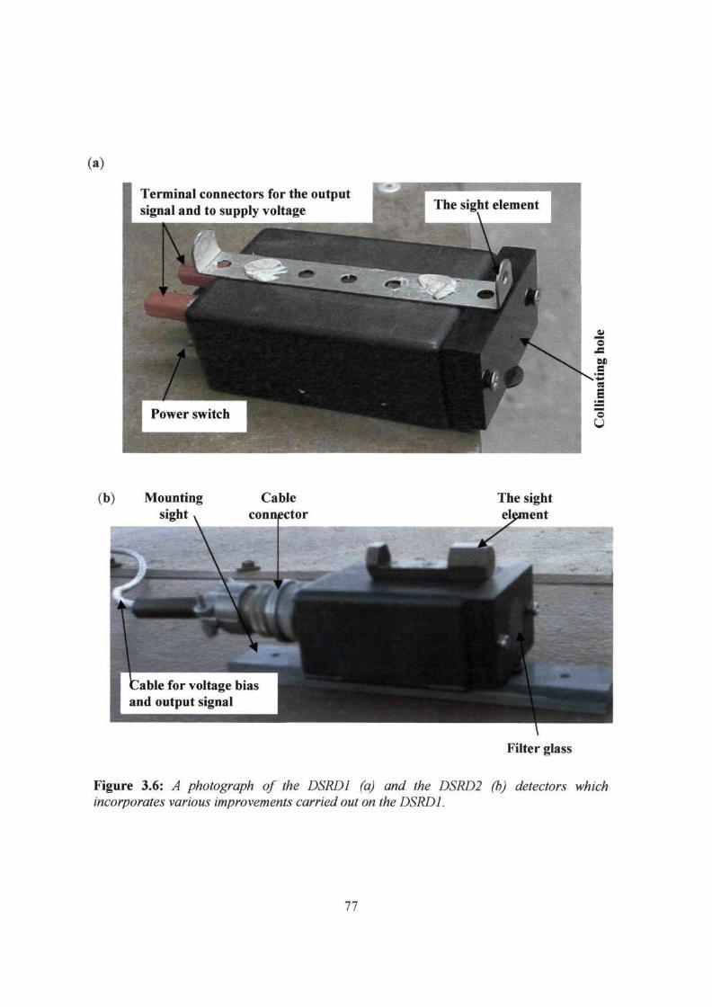
(a)
I erminal connectors for the output signal and to supply voltage
^9 * 8
*
^^F^^l
Power switch
i The sight element
K
— •
?3 i
J ^
ex
Mounting sight
Cable connector
The sight element
Filter glass
Figure 3.6: A photograph of the DSRDl (a) and the DSRD2 (b) detectors which incorporates various improvements carried out on the DSRD1.
77

3.2 Calibration
In general, the goal of a calibration is to correct for small imperfections that are
unavoidable in instruments operating under hostile conditions such as instruments for
solar radiation measurements. A proper calibration of instruments for measuring direct
solar radiation is intended to provide accurate measurements which are very important for
evaluating the performance of solar systems. For example, the accuracy of solar cells
calibrated as primary reference cells is directly dependent on the accuracy of the
pyrheliometer used to measure the direct solar radiation that reaches the solar cell.
Factors that influence the accuracy of pyrheliometer calibrations have been investigated
[Thacher et al, 2000] and it was found that uncertainties of 0.8 % at a level of 2-sigma are
still present.
The DSRD2 was calibrated using a comparison technique with the Eppley NIP whose
characteristics are well known. The direct solar radiation data recorded from both
instruments were plotted on the same graph to establish similarities and differences
between the readings of the two instruments. A correlation factor was determined by
plotting a graph of DSRD2 data against NIP data then fitting a polynomial regression
equation. A best correlation occurs when the polynomial fit gives a root square (R1) equal
to one. A calculation of the error was also carried out. When a correlation is established
the output of the DSRD2 can be converted from a voltage unit into an irradiance unit, in
Wm" since the conversion factor for the NIP is known and is with on the casing of the
instrument as 7.58xl0"6 V/Wm"2.
78

3.3 Experimental procedures
In this section a description is given of the steps followed in carrying out the
measurements of direct solar radiation in order to investigate the characteristics of the
DSRD1 detector.
3.3.1 Installation of the equipment
The equipment required to run the experiment was installed on a deck built on the
rooftop, of the physics building at the University of Kwazulu Natal (Westville Campus).
The roof is -22.5 m high and -325 m above sea level. The site was carefully chosen
taking into account the different aspects that could introduce negative influences to the
measurements. The aspects are listed as follows:
1. No object would cast a shadow over the location at any time during the
measurements in an entire year.
2. To prevent any possible electrical noise interference, the cables from the
instruments to the data acquisition system were made to be as short as possible.
3. All electronic equipment has been installed far away from any sources of
electromagnetic waves.
4. The detectors (DSRD1, DSRD2 and NIP) were mounted on the Eppley sun
tracker that is also mounted onto a rigid stand with good mechanical stability and
well leveled to prevent any movement of the instruments during bad weather
79

days. The stand was solidly fastened to the roof-deck. However, as explained on
page 42, the tracker can be aligned manually to cater for the solstices.
5. It was ensured that a free circulation of the operators and any visitors within the
area would not interfere with the measurements.
6. No reflecting shiny surfaces such as roofs, light poles, white buildings or
buildings with glass are located in the line of sight of the detectors.
7. The detectors were mounted such that there was a clear view of the sun at sunrise
and at sunset.
3.3.2 Data acquisition system
The data acquisition system comprised a Hewlett Packard (HP) data logger model
34970A and a 20 channel multiplexer. The data logger was connected to a desktop
computer via an RS-232 serial port. The software used to enable data manipulation is
Bench Link. The data scanning time interval was set to one second. The connection
between the instruments and the data acquisition system was achieved by a multicolor
cable isolated from possibilities of electromagnetic shocks and rust to prevent electrical
noise. It was also designed to be water-proof.
3.3.3 Measurement procedures
In measuring direct solar radiation, data were acquired using a data logger which was
remotely controlled by a desktop computer using a serial interface. The data logger was
set to scan readings at a time interval of one second and the data were recorded from
SO

sunrise to sunset. The instruments used in the measurement are the DSRDl detector, the
DSRD2 detector and the Eppley NIP and these were mounted together on an Eppley sun
tracker model ST-1. The data capturing was done in the following sequence.
1. A measurement of the direct solar radiation using the DSRDl detector and the Eppley
NIP only. This was intended to find the correlation between the readings of both
instruments, where the NIP served as a reference. A voltage of 9.0 V was supplied
using a 9.0 V battery.
2. The DSRDl detector, the DSRD2 detector and NIP were all mounted together on the
ST-1 tracker. The DSRD2 was fitted with the BG39 optical glass filter. A voltage of
9.0 V was supplied from a 30 V power supply unit.
3. Step 2 was repeated, but with the DSRD2 detector fitted with the KG optical glass
filter.
4. The measurements were performed with no filter on the DSRD2 in order to compare
with the readings of DSRDl taken with no filter.
5. The DSRDl was fitted with first the BG39 filter and then with the KG filter and
measurements taken. The black perspex housing the DSRD2 was replaced with white
perspex for investigation of the effect of temperature.
6. The battery on the DSRDl was replaced with the power supply unit and the DSRD2
was powered from the battery. This is because it was assumed that the output signal
of the DSRDl hai;' been affected by use of the battery as voltage supply.
7. Measurements of temperature in the interior of the detector housing were carried out
using a temperature sensor LM 35 which was located near the sensor of the DSRD2.
81

This sensor is made up of a semiconductor and it gives an output signal in volts,
where 10 mV is equivalent to 1 ° C.
In measuring polar response, measurements were performed as follows:
1. A measurement of direct solar radiation with the instrument aligned properly
assuming this as the zero of angular position with respect to the solar beam. The angle
of incidence was measured using a compass.
2. Data were recorded for different angles between 0 and 40 by varying the angle of
incidence using the line of sight of the sun tracker
82

Chapter 4
Results and Discussion.
In this chapter, the results of the characterization and improvement are presented
together with the results of the calibration. A major part of the measurements were
carried out on averagely clear sky days. This is because it was required that the
instrument be calibrated for clear sky days [Duffie and Beckman, 1991]. On a clear sky
day, fluctuations in direct solar radiation with the time of day are comparable to those
found in the standard solar radiation spectrum measured at sea level. A clear sky day is a
day on which the obstruction of direct solar radiation is negligible. In this case, the
atmosphere is assumed completely transparent to solar radiation. A turbid sky day is a
day on which there are a lot of suspended particles called aerosols that cause a high level
of scattering of solar radiation. The atmosphere is then assumed to be an opaque body
through which no light passes.
The detection principle of the DSRD is based on direct conversion of the incident solar
energy into a current which is then converted into a voltage. This is achieved by
connecting an amplifier as a transimpedance on the integrated circuit of the DSRD. A
resistance connected across the thermopile output converts the current produced at the
83 i

junction into a voltage. Thus, the output of the DSRD is a voltage signal. The output of
the NIP is also a voltage signal. The conversion of energy in both detectors into a voltage
signal is to enable the data logger to take readings directly from the detector. The
magnitude of the output signal given by both DSRD1 and DSRD2 is of greater order
compared to the magnitude of the output signal given by the reference instrument, the
NIP. This is because the gain of the DSRD is greater than the gain of the NIP because the
DSRD has a higher-gain amplifier incorporated in the circuit (see page 62). This situation
has been corrected by calibrating the DSRD. The plot of direct solar radiation data
collected using the NIP is indicated with the blue curve, while the plot of data collected
with the DSRD1 is indicated with the red curve and the plot of data collected witfi the
DSRD2 is indicated with the pink curve.
The NIP, being the reference instrument, is very important and deserves a brief
description of its characteristic response to solar radiation. The trace shown in Fig.4.1 is a
plot of direct solar radiation measured in volts with the NIP during a clear sky day.
Before 07:00 the graph suggests that there is no variation in the amount of solar energy
measured because it is before the sun rises. This occurs because the detection principle of
the NIP is based on the difference in temperature between the junctions of the thermopile
and its sensing element. After sunrise, the instrument absorbs solar energy and this causes
a rise in temperature which produces an electrical current that can be measured as a
voltage.
84

The graph of Fig. 4.1 also shows that the instrument gives negative values just before
sunrise. The data logger was programmed to commence the recording process at 06:45
which was the estimated sunrise for that day. The negative readings suggest that the
temperature difference on die junction of the thermocouple is negative and the sensing
element is not absorbing energy but releasing it since there is no sun.
I
7.0
6.0
5.0
4.0
g 3.0 K —1
g 2.0
1.0
0.0 -1.0
DATE 09/07/04
_ u
/
/
/
/
f f
V \J ^\* *v >
N \
1
\ \
y
\
\
6.0 7.0 8.0 9.0 10.0 11.0 12.0 13.0 1l0 15.0 16.0 17.0 TIME (Hi
NIP
Figure 4.1: A graph of direct solar radiation measured in volts using the NIP. The graph depicts the variations of the amount of solar energy that is available for a particular day.
85

Another possible source of this fault in the instrument is the fact that it has not been
calibrated since it was shipped in 1996 [Dhavraj, 1998]. This apparent weakness of the
instrument is not expected to affect the results much though.
4.1 The DSRDl and the NIP on a clear day
An experiment was conducted in order to investigate a general behavior of the DSRDl
detector in terms of its response to variations of solar radiation in comparison to the NIP.
The data were taken on different days but under clear sky conditions. Four sets of
measurements were performed, firstly with no filter, then with the KG filter, thirdly with
the BG39 filter and finally using a power supply. The results are presented below.
4.1.1 The DSRDl (with no filter) and the NIP
A concern and a most important aspect of the experiment is the way that the DSRD l
readings track the variation of solar radiation as given by the reference instrument. The
results are shown in Fig. 4.2. The red curve represents a plot of direct solar radiation in
volts measured using the DSRDl and the blue curve is a plot of direct solar radiation also
in volts, measured using the reference instrument, the NIP. The measurements were taken
on 25th June 2004.
The scaling on the vertical axes is different due to the difference in magnitude between
the readings of the DSRDl and the NIP, the DSRDl readings being about six times those
86

of the NIP. The same axis system is used to enable a comparison in terms of how the
measurements taken with the DSRDl track the characteristic variations of solar radiation
according to measurements obtained from the NIP.
6.0 -
C en > 5.0 -
J. 8 4.0-< t-O 3.0 ->
z 2 0 -
1.0 -
n n -U.U 1
DATE 25/06/04
w^
/
> « * • "
/ f
?£ •
•U
^ * • n , % V)
\n t * i
^ H
; \ • - .
" >
*w-"
r —***
v \
-"*
\
\
1
\
\
NIP
-DSRD1
- 35.0
- 30.0 >
- 25 0 g
• 22 ° 5 - 150 5
5 - 10.0 S
- 5.0
n n — • u
8 9 10 11 12 13 14 15 16 17 TIME (H)
Figure 4.2: A plot of direct solar radiation measured in volts using the DSRDl (with no filter) and the reference instrument, the NIP. Here, ,he vollage applied to the DSRD1 was supplied from a 9.0 V battery.
The graph of the reference instrument (blue) shows an increase in solar radiation intensity
from sunrise to about 11:30 after which it starts to decrease until sunset at about 16:30.
For a clear sky day this is the expected behavior of the variation in direct solar radiation
intensity measured at sea level, taking into account the attenuation of solar radiation. In
contrast, the graph of direct solar radiation measured using the DSRDl shows no
87

significant variations in intensity between about 07:30 and 15:30, after which it shows an
increase towards sunset. This is a clear indication of malfunction of the DSRDl detector
for measuring direct solar radiation mainly since it should read zero at sunset. Because
there is more IR radiation towards sunset, it means that the DSRDl is more sensitive to
this type of radiation. The first filter used is thus aimed at cutting off this radiation.
4.1.2 The DSRDl (with filter KG) and the NIP
The attempt to correct the spectral response of the DSRDl was by the use of a cut-off
glass filter, KG. The results of the performance of the DSRDl combined with the filter
are indicated in figure 4.3. These measurements were taken on 19 July 2004.
6.0 -
> 5.0 -
$ 4 . 0 -
f j 3.0 -> 1 . 0 -
1.0 -
nn .
DATE 19/07/04
/ f S**
Sr* ^^H E£J <wft >*J*'
V*» • K ^
%
N ^
\ \
•^•f^
™
\
ft
\
1
\
\
. 1
1
\
' 8 9 10 11 12 13 14 15 16 1
TIME (H)
NIP -DSRD1
- 0.30 g
rs - 0.20 ^
> a g v>
- 0.10 a
- n nn
7
Figure 4.3: A plot of direct solar radiation measured in volts using the DSRDl (coupled to KG filter) and the NIP. A 9V battery was used as the voltage supply. (Note that the left scale is given in V))
88

Figure 4.3 shows no significant difference in the readings given by DSRDl except that
towards sunset the results now indicate a decrease in direct solar radiation received. This
is contrary to the results plotted in Fig. 4.2. Another observation is that the magnitude of
the signal from the DSRDl has decreased dramatically by 2 orders of magnitude. The
effect of IR radiation as indicated in figure 4.2 is not present here, which suggests that the
filter is working to prevent IR radiation from the detecting element.
4.1.3 DSRDl (with filter BG39) and the NIP
Figure 4.4 is a plot of solar radiation measured with the DSRDl (coupled to the BG39
filter) and the NIP. The voltage is still supplied from the 9.0 V battery.
7 0 •
6.0 J
5.0 •
— 4.0 UJ
«> I - 3.0 • _ l
o > 2.0 • z
1.0 •
0.0 •
1 n . -1 .U 1 j
i DATE 13/08/04
/
r** <** %4\,
"**•> **f
i
s* \
%
\
\
\
\
y \
S 9 10 11 12 13 14 15 16 17 1
TIME (H)
NIP
— DSRD1
• 0.40
• 0.30 ,—.
LU
a 3 v>
• 0 10
r 0.00 8
Figure 4.4: A plot of direct solar radiation measured in volls using the DSRDl (coupled to the BG39 filter) and the NIP. The voltage was supplied from a 9.0 Vbattery.
89

The plot indicates that the spectral response of the detector has been modified although it
is still not tracking the variations of the direct solar radiation properly as shown by the
results from the reference instrument. At 09:00 and at 09:30 the solar energy measured by
the DSRD1 increased abruptly before leveling off followed by another rapid decrease.
These results disagree with those given by the reference instrument. However, the results
indicate that the filter is working to block out IR radiation.
4.1.4 The DSRD1 (using a power supply, with no filter) and the NIP
The measurements were performed with a 30 V power supply unit in place of the 9 V
battery. Figure 4.5 shows the results of these measurements which were taken with no
fin
7.0 -
~ 6.0 -E m 5 - ° -
£ 4.0 -
> 3.0 -a. 5 2.0 -
1.0 -n n J
E
DATE 30/07/04
i 1 f -
1/ -1
j i
% h
*
^^ * *
*k
•>%!*•
10
• ^ %
* •*
""\ i - " -> i V
U« *C V
**
\ V
s
\
s
\ \
*\
\
\ \
J 9 10 11 12 13 14 15 16 17 1
TIME (H)
— NIP - DSRD1
- 0.09
- 0.08
- 0.07 J 5
- 0.06 < t-
• 0.05 S
-0.04 g • 003 * - 0.02 ° - 0.01
. n nn 8
Figure 4.5: A plot of direct solar radiation measured in volts using the DSRD1 (with no filter) and the NIP. The voltage was supplied from a 30 V power supply unit.
90

inter. The data were taken on JU July AI04. This plot reveals no improvement in the
readings given by DSRDl. In contrast to the readings of the reference instrument, the
readings of the DSRDl suggest a turbidity in the sky between 08:45 and 11:00.
Moreover, from 12:30 the readings of the DSRDl suggest an increase of the amount of
detected solar energy. Both of these results disagree with the readings of the NIP, and this
can be attributed to the electrical noise associated with the power supply unit.
4.2 The D S R D l and the NIP on a turbid day
On a turbid day, the scattering of the solar beam is higher and the amount of solar energy
received on the earth's surface is lower and should show a predominance of infrared
radiation.
4.2.1 The DSRDl (with no filter) and the NIP
A presentation of direct solar radiation measured in volts using the DSRDl detector and
the NIP on a turbid day is shown in figure 4.6. The NIP readings reveal significant
fluctuations in solar radiation intensity around noon and this means that during this
period there was some interference that could be a spontaneous cloud cover or a
spontaneous turbidity. However, the readings of the DSRDl indicate no considerable
variations in the amount of solar energy received during this period. Also, in contrast to
the reference instrument, between 08:30 and 09:30, the readings suggest a decrease while
from 16:00 the readings suggest an increase in the amount of solar energy received. The
data were taken on 22n<t July 2004.
91

R n
5.0 -
> £.4.0 -LU © £ 3.0 -d J 2.0 -z
1.0 -
n n -U .U 1
DATE 22/07/04
_ i i 1 /
h
/
Mi
y •*•* i *U^ " \
1l w r 1
inv »v w*,
I t — t - i .
\ ,
\
* 1
1 1 \
l
NIP -DSRD1
• 0.09
• 0.08 ~
• 0.07 iu 0
• 0.06 < i -
• 0.05 o
• 0.04 ^
• 0.03 g • 0.02 Q
• 0.01 . n nn
) 9 10 11 12 13 14 15 16 17 18
TIME(H)
Figure 4.6: A plot of direct solar radiation measured in volts using the DSRDl and the reference instrument, the NIP. The voltage was supplied from a 9.0 V battery and the DSRDl incorporates no filter.
4.1.3 The DSRDl (with the KG filter) and the NIP
In Figure 4.7, the results of the direct solar radiation measured in volts using the DSRDl
detector incorporating the KG filter on a day with a turbid atmosphere, are presented. The
voltage was supplied to the DSRDl from a 30 V power supply unit. Here, the
interference occurred for almost the entire day with more significance between sunrise
and -09:00 and later between 13:00 and -15:30. An error in the data acquisition system
occurred that necessitated an interruption on data scanning just before sunset, hence the
lack of data from about 15:00. The measurements were taken on 5th October 2004.
92

6.0 -
> 5.0 -
$4 .0 -
^ 3 0 ->
| .,0 -
1.0 -
n n . U.U i
E
DATE 05/10/04
^l« 1 7
T f
H I I L
./*• f r r n I
r -s. 11 >1
3 3
L 1
1 111
in.
\ }
MP -DSRD1
inn
- 9 0
- 8.0 ^
- 7.0 UJ
o - 6.0 £ - 5 0 S
> - 4 0 5 -30 *
- 2.0 °
- 10 _ n n
8 9 10 11 12 13 14 15 16 17 18 riME (H)
Figure 4.7: A plot of direct solar radiation measured in volts using the DSRDl and the NIP on a turbid day. The DSRDl incorporates the KG filter and the voltage is supplied from the 30 Vpower supply unit (note that the left scale is given in V))
A comparison of the DSRDl results and the NIP results reveals that the readings of the
DSRDl do not follow the variations in the amount of solar energy that reaches the earth's
surface as indicated by the reference instrument. However, the detection of IR radiation,
the predominant radiation during periods of intense scattering like on a turbid day, seems
to be eliminated. For instance, this is indicated in the turbid period between -07:00 and
-08:15 where the red trace shows a minimum.
93
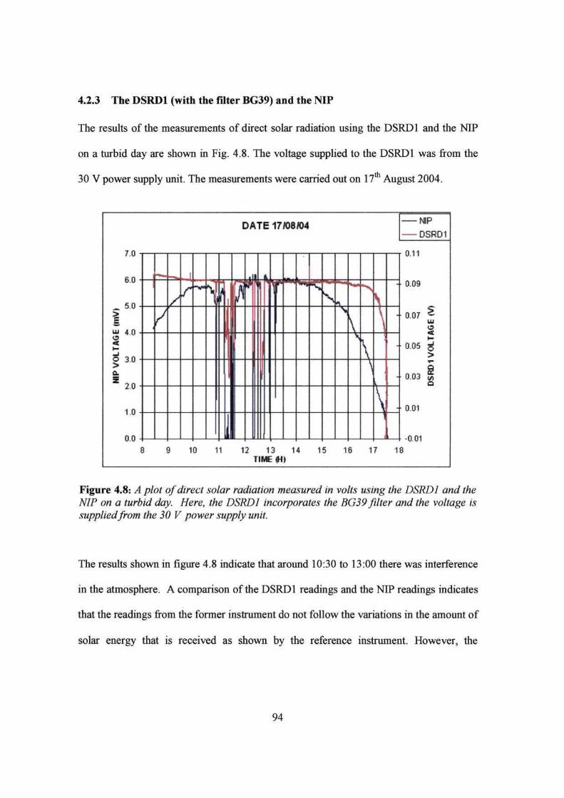
4.2.3 The DSRDl (with the filter BG39) and the INIP
The results of the measurements of direct solar radiation using the DSRDl and the NIP
on a turbid day are shown in Fig. 4.8. The voltage supplied to the DSRDl was from the
th 30 V power supply unit. The measurements were carried out on 17 August 2004.
6.0 -
_ 5.0 -
Iw 4.0 -a < t—
0 3.0 -
1 2 .0-
1.0 -
n n .
(
DATE 17/08/04
/
/ r " V
\t _ iit1
.L I
j 1 9 10 11 12
TI
i
V
-
-
13 14 15 16 17 1 riE (H»
NIP
- DSRD1
r 0.11
0.09
0.07 S Ul
0.05 £ >
9 0.03 o
a
0.01
. -ft ni 8
Figure 4.8: A plot of direct solar radiation measured in volts using the DSRDl and the NIP on a turbid day. Here, the DSRDl incorporates the BG39 filter and the voltage is supplied from the 30 V power supply unit.
The results shown in figure 4.8 indicate that around 10:30 to 13:00 there was interference
in the atmosphere. A comparison of the DSRDl readings and the NTP readings indicates
that the readings from the former instrument do not follow the variations in the amount of
solar energy that is received as shown by the reference instrument. However, the
94

detection of IR radiation has been eliminated as shown by the lack of increase in voltage
at around sunrise and sunset.
The overall results from the DSRDl measurements reveal several aspects. Firstly, in both
figures 4.2 and 4.3 the graphs show nearly similar characteristics. This is as if the amount
of direct solar energy was increasing at near sunset times. For those situations when the
DSRDl incorporates an optical glass filter, a kind of malfunction is revealed. These
results suggest that the detector sensitivity is more pronounced in relation to IR radiation
since this type of radiation is predominant at sunset. Another observation is that the
DSRDl responds equally during the day, especially over the period when solar radiation
should reach a peak value. This suggests that this poor correlation could be due to some
alteration of the original characteristics of the detector, which could have caused by
exposure to moisture and dust. It is for this reason that the DSRD2 detector was built
using a sensing element with the same characteristics.
4.3 The DSRD2 and the NIP on a clear day
This section is a presentation of the results of the various improvements carried out on
the DSRDl with respect to the spectral response. The improvement is focused on
coupling a glass filter to the detector to give an overall response. It is hoped that the
response will better characterize the amount of direct solar energy received on the earth's
surface especially on a clear sky day. The results are presented first, for the case with no
95

filter and then for the two cases when the detector is coupled to the two different filters.
As mentioned earlier the blue trace represents data collected with the NIP and the pink
trace, the data collected with the DSRD2.
4.3.1 The DSRD2 (with no filter) and the NIP
The DSRD2 was mounted together with the NIP on the sun tracker for a comparison of
their responses. A plot of direct solar radiation measured in volts using the DSRD2 and
the NIP is shown in Fig. 4.9.
fi n _ 3.U
4.0 -
< t -_i O 2.0
> z
1.0 -
nn . U.U H
(
DATE 22/07/04
1
f 1 ft to w ^
y^ s i
\ v
1
1 9 10 11 12 13 14 15 16 1
TIME (Hi
MP
- DSRD2
F 1 Q I o
• IB
-1.4 E
• 1 2 g
•1.0 £ o
• 0 8 >
• 0 6 £
•0.4 °
• 0.2
. n n r UU
7
Figure 4.9: A graph of direct solar radiation measured in volts using the DSRD2 and the NIP. The voltage to the DSRD2 detector was supplied from the 30 V power supply unit.
96

The blue curve represents the measurements of taken with the NIP and the pink curve
represents the measurements taken with the DSRD2. The data indicates that the DSRD2
with no filter tracks the variations of direct solar radiation in a similar manner as the
reference instrument. Since the sensing element is the same in both detectors, this means
that the optical properties of the sensing element on the DSRDl detector must have been
altered. This may have been caused by moisture and dust that could have accumulated in
the housing and onto the surface of the sensor. This could have happened because the
housing of the DSRDl is not properly sealed. However, the DSRD2 graph does not
exactly follow the NIP graph especially just before midday where the NIP reads higher
than the DSRD2.
The fact that the readings of the DSRD2 between ~-08:45 and ~12:15 are lower than the
readings of the NIP suggests that the response of the sensor in the DSRD2 is dependent
on the wavelength o2 solar radiation. This means that the DSRD2 responds better to
radiation at near infrared region, which occurs in the period from sunrise until -09:00 and
from around 15:00 when the sun moves towards sunset. However, the traces indicate that
even if the correlation is not good, tlie detecting device can be used to measure direct
solar radiation with a reliable accuracy.
Figure 4.10 shows the plot of correlation between readings taken with the DSRD2 and
those taken with the NIP. Also shown in red is a curve fit to the data and this can be used
to correct the small imperfections on the readings of the DSRD2 that are observed from
97

the plot. The plot shows a significant deviation of the calibration curve in relation to the
plot of correlation from 1.5 mV of the NIP voltage.
iscor1
1600 -
1400 -
1200
| JJLJ 1 0 0 0
•si > 800
H cm
400 '
200
2 2.5 3 NIP VOLTAGE (mV)
Figure 4.10: 4 graph of correlation between the DSRD2 and the NIP measurements. The red curve represents the calibration factor which must be taken into account to correct the readings of the DSRD2 in order that they agree with those from the reference.
The calibration curve displayed is a well-known and long-established polynomial
function of me 8 order estaDiished from mat 01 first order (a linear equation
asbx1 +c = y) and that of second order (a quadratic equation as ax2 +&r + c =y) and
so on. It is given by
P - P^x +P2x +P2x +P4* +Psx*+P6x +P7x +P%& + P9 (4.1)
98
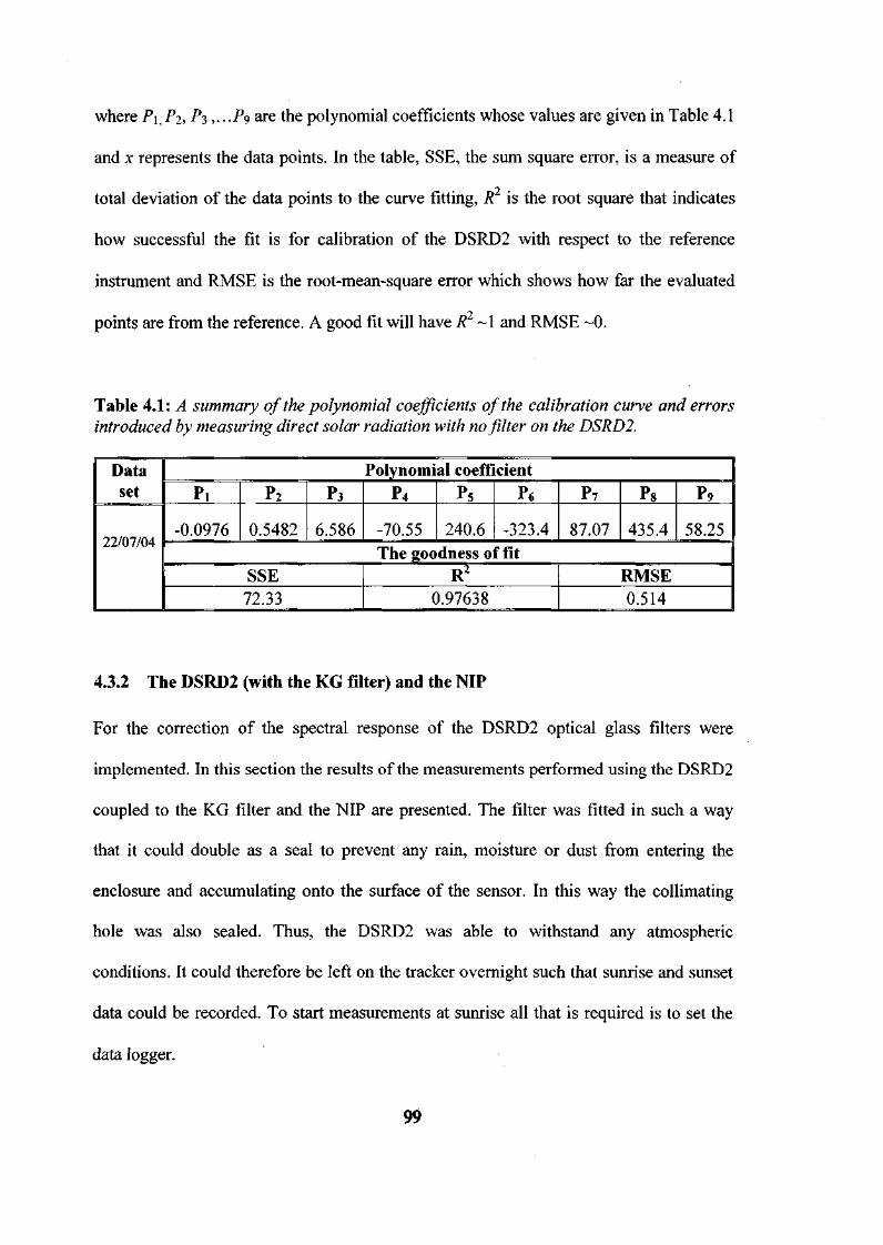
where P\tPi> Pi >-.-P9 are the polynomial coefficients whose values are given in Table 4.1
and x represents the data points. In the table, SSE, the sum square error, is a measure of
total deviation of the data points to the curve fitting, R is the root square that indicates
how successful the fit is for calibration of the DSRD2 with respect to the reference
instrument and RMSE is the root-mean-square error which shows how far the evaluated
points are from the reference. A good fit will have R ~1 and RMSE ~0.
Table 4.1: A summary of the polynomial coefficients of the calibration curve and errors introduced by measuring direct solar radiation with no filter on the DSRD2.
Data set
22/07/04
Polynomial coefficient Pi
-0.0976
P 2
0.5482
P3
6.586
P4
-70.55
Ps
240.6 The goodness ol
SSE 72.33
P«
-323.4 ffit
R2
0.97638
P 7
87.07
Ps
435.4
P 9
58.25
RMSE 0.514
4.3.2 The DSRD2 (with the KG filter) and the NIP
For the correction of the spectral response of the DSRD2 optical glass filters were
implemented. In this section the results of the measurements performed using the DSRD2
coupled to the KG filter and the NIP are presented. The filter was fitted in such a way
that it could double as a seal to prevent any rain, moisture or dust from entering the
enclosure and accumulating onto the surface of the sensor. In this way the collimating
hole was also sealed. Thus, the DSRD2 was able to withstand any atmospheric
conditions. It could therefore be left on the tracker overnight such that sunrise and sunset
data could be recorded. To start measurements at sunrise all that is required is to set the
data logger.
99
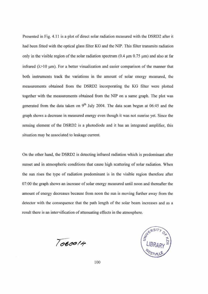
Presented in Fig. 4.11 is a plot of direct solar radiation measured with the DSRD2 after it
had been fitted with the optical glass filter KG and the NIP. This filter transmits radiation
only in the visible region of the solar radiation spectrum (0.4 urn 0.75 urn) and also at far
infrared (A>10 um). For a better visualization and easier comparison of the manner that
both instruments track the variations in the amount of solar energy measured the
measurements obtained from the DSRD2 incorporating the KG filter were plotted
together with the measurements obtained from the NIP on a same graph. The plot was
generated from the data taken on 9th July 2004. The data scan begun at 06:45 and the
graph shows a decrease in measured energy even though it was not sunrise yet. Since the
sensing element of the DSRD2 is a photodiode and it has an integrated amplifier, this
situation may be associated to leakage current.
On the other hand, the DSRD2 is detecting infrared radiation which is predominant after
sunset and in atmospheric conditions that cause high scattering of solar radiation. When
the sun rises the type of radiation predominant is in the visible region therefore after
07:00 the graph shows an increase of solar energy measured until noon and thereafter the
amount of energy decreases because from noon the sun is moving further away from the
detector with the consequence that the path length of the solar beam increases and as a
result there is an intersification of attenuating effects in the atmosphere.
'£ -A £ *\
t /ft N 1 UBRARY J / 0600/4*
100
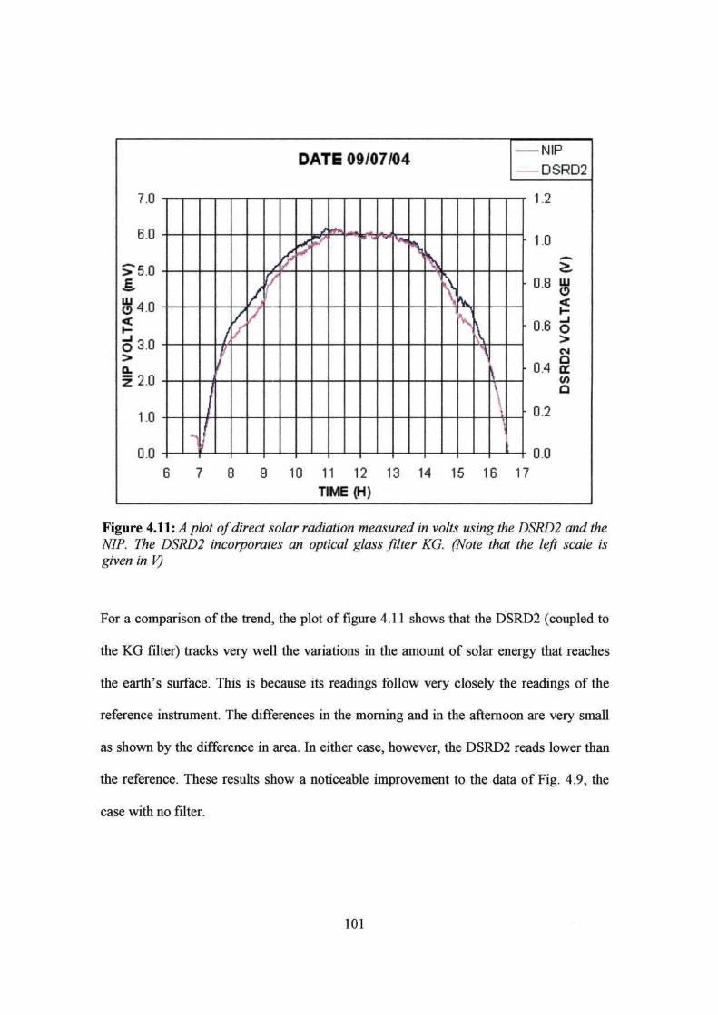
7.0 •
6.0 -
>5.0 -
£ $4 .0 -< O 3.0 -> Q.
z 2.0 -
1.0 -
0.0 i E
DATE 09/07/04 •
1
/ /
/
r
r U /
(
r "" ^ 1 •" *
V 1 f\ s
\ \
\
NIP
-DSRD2
!
• 1.2
• 1,0
• 0 8 g <
• 0.6 o >
- 0.4 tr to a
• 0.2
1 0 . 0
i 7 8 9 10 11 12 13 14 15 16 17 TIME (H)
Figure 4.11: 4 plot of direct solar radiation measured in volts using the DSRD2 and the NIP. The DSRD2 incorporates an optical glass filter KG. (Note that the left scale is given in V)
For a comparison of the trend, the plot of figure 4.11 shows that the DSRD2 (coupled to
the KG filter) tracks very well the variations in the amount of solar energy that reaches
the earth's surface. This is because its readings follow very closely the readings of the
reference instrument. The differences in the morning and in the afternoon are very small
as shown by the difference in area. In eiuier case, however, the DSRD2 reads lower than
the reference. These results show a noticeable improvement to the data of Fig. 4.9, the
case with no filter.
101

For a comparison of the magnitude of the readings obtained from the two instruments, the
values of the measurements obtained from the DSRD2 were corrected to the
measurements obtained with the NIP as determined from figure 4.11. This correction
factor is 171.429 and the result is shown in figure 4.12. The difference between the
readings is, however, lower and this indicates that the DSRD2 reads closer to the
reference. The correction factor was evaluated first by the ratio between the DSRD2
measurements and the measurements from the NIP for each corresponding data point.
Secondly, an average of the ratio values was calculated and this was used to divide into
each data point. The result from this division was used in the plot in Fig. 4.12 and has
been evaluated as 171.429.
i n •
/.u
6.0 -
5.0 -
> £ 4.0 • H j j 3.0-O 2.0 ->
1.0 -
0.0 -11) 4
- 1 .U 1 t
DATE09W7/04
- n
/
/
/
/
r f
S
rf r*
' • • * ! i
*< A "S
V
\ 1 \
I
J 7 8 9 10 11 12 13 14 15 16 1
TIME(H)
NP DSRD2
7
Figure 4.12: A plot of the direct solar radiation measured in volts using the DSRD2 and the NIP. This plot indicates a characteristic behavior of the variation of solar energy on a clear atmospheric conditions day.
102

A comparison between the graphs in Fig. 4.12 indicates that the DSRD2 reads lower in
the period that extends from 07:45 until 11:00 and also between 14:15 and 16:00. The
reason for this difference is associated with the fact that the combined spectral response
of the sensing element and the KG filter (according to Fig. 3.5) varies with respect to the
wavelength of solar radiation. Nevertheless, the use of the optical glass filter KG has
improved the spectral response compared to the case when no filter was used.
Figure 4.13 is a plot of correlation between data obtained from the DSRD2 incorporating
the KG filter and the data from the NIP showing also the calibration curve.
i i > t *
NIP VOLTAGE (mV)
Figure 4.13: A graph of correlation between the DSRD2 ami the NIP measurements, the red curve represents the calibration factor which must be taken into account to correct the readings of the DSRD2 in order that they agree with those of the reference.
101

The figure reveals tha+ the readings of the DSRD2, when fitted with the KG filter, tracks
comparatively with the reference. The figure also shows a good curve fit for calibration
of the DSRD2 since the calibration curve follows very well the correlation curve. There
is better agreement in this case than there was in Fig.4.10. This calibration curve is also a
polynomial function of 8t order as evaluated by Eq. (4.1), with coefficients given in
Table 4.2. The two lines displayed in Fig. 4.13 are due to the nearly parabolic form of the
graphs in Fig. 4.12 anC this causes a duplication of data points in the correlation curve.
Table 4.2: A summary of the polynomial coefficients of the calibration curve and errors introduced by measuring direct solar radiation with the DSRD2 incorporating the KG filter.
Data set
09/07/04
Polynomial coef Pi
0.013
P2
-0.185
P3
0.060
P4
9.762
Ps
-53.81
icient
P6
97.31
P7
-23.81
P8
100.1
p9
26.84 The goodness of fit
SSE 0.4112
R2
0.99878 RMSE 0.0976
The value of R-square is nearly equal to unity and this means that the readings given by
the DSRD2 incorporating the KG filter are nearly equal to those given by the reference.
In other words, this combination of the DSRD2 and the KG filter provides a better
characterization of direct solar radiation which nearly mimic the reference instrument.
The value of the root-mean-square error is nearly equal to zero and this means that the
deviation in relation to the reference can be considered as negligible.
104

4.3.3 The DSRD2 (with the BG39 filter) and the NIP
In this section the results presented refer to the measurements acquired using the DSRD2
after it was fitted with the optical glass filter BG39. This filter transmits solar radiation in
the wavelength range between 0.32 and 0.70 urn. Presented in Fig. 4.14 are the
measurements obtained from the DSRD2 (fitted with the BG39 filter) and the NIP. The
data were taken on 25 June 2004.
6.0 -
> 5.0 -it
8 4.0-< O 3.0 -> a. Z 2.0 -
1.0 -
n n -
DATE 25/06/04
fc"*V ^Vi 7 \»
• \
"S > V
*
\
1 \
8 9 10 11 12 13 14 15 16 1 TIME (H)
NIP -DSRD2
, n c U.D
- 0.5
-0.4 g
- 0.3 o >
- 0.2 § v> a
- 0.1
- n n r U.U
7
Figure 4.14: A plot of direct solar radiation measured in volts using the DSRD2 and the NIP. The DSRD2 is fitted with the BG39 filter and the voltage is supplied from the 30 V power supply unit.
The plot is a presentation of data obtained on a clear sky day. As can be seen from the
figure, minor variations in the amount of solar energy detected are recorded and these are
105

radomly caused by atmosoheric conditions. On a clear sky day like the case shown in the
figure, the amount of solar energy recorded by the NIP and the DSRD2 increases as the
sun approaches the detector with a peak at noon. The DSRD2 voltage is about two orders
of magnitude higher than the NIP voltage. In general, the graph of Fig. 4.14 indicates that
die DSRD2, when fitted with the BG39 filter, produces a signal that follows the
variations in the amount of solar energy as measured by the NIP at the earth's surface and
even records die occurrence of spontanious interference. As seen in the previous sections,
6.0 •
5.0 •
I * 4 . 0 -(T
J 3.0• o >
2.0 •
1.0 •
0.0 •
DATE 25/06/04 t
/
/
/
1 f
/ •** "" ^
*% "*+) N*
" *n >y
V
^ N \ 1 \
•
•
1
i 8 9 10 11 12 13 14 15 16 1'
TIME (H)
NIP
DSRD2
f
Figure 4.15: 4 plot of direct solar radiation measured in volls using the DSRD2 and the NIP on a clear sky day. The DSRD2 incorporates the optical glass filter BG39, and the DSRD2 data have been corrected to the NIP data by 85.714.
106

the magnitude of the signal obtained with the DSRD2 is higher than that obtained with
the reference instrument. In order to compare the trend and the magnitude, the data
obtained from the DSRD2 are corrected to the NIP data by multiplying by 85.714. This is
shown in Fig. 4.15
There is generally good agreement between the DSRD2 and the reference except at two
regions starting around 10:00 and 14:00. In the former case the DSRD2 reads lower than
the reference, while in the latter case it reads higher. This shows that the DSRD2 fitted
with the BG39 filter has less sensitivity to direct solar radiation during a period in which
the predominant radiation is of a wavelength of -0.45 pm. This is towards the time of
maximum solar irradiance when the sun is at the closest position in relation to the
detector. In the later case, the DSRD2 has higher sensitivity in the afternoon, a period
leading towards maximum temperature when the earth is beginning to irradiate more of
the absorbed radiation.
A plot of the correlation curve between the data obtained with the DSRD2 incorporating
the BG39 filter and data obtained by the NIP is given in Fig.4.16 together with the fitting
curve for calibration of the DSRD2. The graph reveals discrepancies between the
correlation curve and fhe fitting curve. In other words, the fitting curve does not follow
the correlation curve. This suggests that a combination of the DSRD2 and the BG39 filter
is not good for measuring direct solar radiation since it has poor agreement with the
reference instrument. The second blue line appearing at higher NIP voltages can be
explained for similar manner as in Fig. 4.13. The correlation coefficients and the errors
107

are summarized in Table 4.3 and the values indicate that a better correlation between the
DSRD2 and the NIP is achieved when the former detector incorporates a filter than when
without it. However, the R-square value obtained with the KG filter is closer to unity than
that obtained with the BG39 filter.
' ' ' ,—i 1 r
NIP VOLTAGE (mV)
Figure 4.16 A graph of correlation between the DSRD2 (incorporating the BG39 filter) and the NIP measurements. The red curve represents the calibration factor which must be taken into account when correcting the readings of the DSRD2 in order that they are of same magnitude as those from the reference.
108

Table 4.3: A summary of the polynomial coefficients of the calibration curve and errors introduced by measuring direct solar radiation with the DSRD2 incorporating BG39 filter.
Data set
22/07/04
Polynomial coefficient Pi
0.011
p2
2.844
1*3
-30.44
P4
170.4
Ps
-530.9
P6
900.7
P7
-735.8 The goodness of fit
SSE 2.228
R2
0.98344
P8
282.7
RMSE
P9
-10.9
0.1454
The RMSE value is more closer to zero in first case than in the second case. This means
that a better combination between the DSRD2 and the filter is achieved with the KG filter
than with the BG39 filter. Comparing R-square and RMSE values from all three tables
shows that the performance of the DSRD2 is better when it has a filter coupled to it.
Table 4.4 summarizes the values of R-square and RMSE for these three situations.
Table 4.4: A summary of the goodness of the correlation between the readings of the DSRD2 and the NIP for the three situations presented above for a clear sky day.
DSRD2 With no filter With the KG filter With the BG39 filter
SSE 72.33 0.4112 2.228
R 0.97638 0.99878 0.98344
RMSE 0.5139 0.0976 0.1454
4.4 The DSRD2 and the NIP on a turbid day
Measurements of direct solar radiation with the DSRD2 on a turbid sky day were also
performed. The data has, however, not been used in the calibration of the DSRD2, rather
it has been used to give an indication of how good the response of the DSRD2 to direct
109

solar radiation is in other sky conditions. This means that the graphs of correlation as well
as the coefficients for each situation are presented merely to evaluate the goodness and
the reliability of the readings obtained from the DSRD2 and the suitability of each optical
glass filter investigated.
4.4.1 The DSRD2 (with no filter) and the NIP
Measurements of direct solar radiation with the DSRD2 (with no filter) for a turbid sky
day are presented in Fig. 4.17. The measurements were taken on 23r July 2004, and the
DSRD2 signal is about 33.33 times larger than that of the NIP.
e n
5.0 -
> J. 4.0 -m O £ 3.0 -_ i O i 20-z
1.0 -
n n -U U i
E
DATE 23/07104
_JL
7 /
/
s" ^ * f" mm A ift"
^ iii
fi ita to
f* f
pi I P
/ s
\ \
V
\ '
\
) 9 10 11 12 13 14 15 16 17 1
TIME (H)
NIP DSRD2
2 00
- 1.80
• 1 60 ^
- 1.40 m O
- 1.20 -C H
- 1.00 o
-0.00 CM
a - 0 60 * - 0 40 ° - 0 20
. n nn r u.UU 8
Figure 4.17: A graph of direct solar radiation measured in volts using the DSRD2 and the NIP on a turbid sky day. The DSRD2 incorporates no filter.
110

The figure shows that from about 10:00 up to 16:00 there occurred a significant variation
of direct solar radiation incident onto the detector and this suggests that the sky was
turbid. An important observation is that the DSRD2 keeps tracking the variations in direct
solar radiation and follows closely the NIP curve. Although readings from the DSRD2 in
this plot appear to be following the readings of the NIP, the data can not be used for
calibration. This is because the WMO recommends mat any calibration of radiometers
must be carried out under clear sky conditions [Duffie and Beckman, 1991].
In Figure 4.18 the DSRD2 data has been corrected to the NIP data for a comparison of
their magnitudes.
DATE 23/07/04
c n o i l
5.0 •
5-4.U •
J, UJ
2 0 •
i n . 1 0
n n .
7
si r\
t*M «1
l iri i
\
V \
\
\
1
NIP
DSRD2
8 9 10 11 12 13 14 15 16 17 13
TIME (H)
Figure 4.18: A plot of direct solar radiation measured in volts using the DSRD2 and the NIP on a turbid day. Here, the magnitude of the signal acquired with the DSRD2 was corrected to that of the signal acquired with the reference instrument. The DSRD2 incorporates no filter.
I l l

As seen from the figure the magnitude of the signal obtained from the DSRD2 is greater
than that of the signal obtained from the reference instrument.
For correction of the measurements obtained from the DSRD2, the procedures are as
explained in section 4.3.1. Of interest in the figure is that before 13:00, the NIP reads
much higher than the DSRD2. In the afternoon the magnitudes are comparable.
Figure 4.19 is a plot of correlation between the DSRD2 (with no filter) and the NIP
readings on a day when the sky was turbid. The curve fit is a polynomial function of 8
order as in Eq. (4.1). This fitting curve does not track the correlation curve and this
1 ' * * * * f
11 i j j j j i 0 1 2 3 4 5 6
NIP VOLTAGE (mV)
Figure 4.19: A graph of correlation between the DSRD2 and the NIP on a turbid day. The DSRD2 incorporates no filter and the red curve represents the calibration factor that woull be taken into account to correct the readings of the DSRD2 to those of the reference.
112

suggests a significant level of error as evinced by the large difference in magnitudes up to
about 15:00. The polynomial coefficients corresponding to the plot of Fig.4.19, are
presented in Table 4.5 were trie K value is close to unity but the RMSfc value is much
higher than zero.
Table 4.5: A summary of the polynomial coefficients of the calibration curve and the errors introduced by measuring direct solar radiation with the DSRD2 with no filter on a turbid day.
Data set P i P2 P3
Polynomial coefficient P4 _Pj_ P6 P7 J**L P9
23/07/04 0.269 -6.039 54.00 -242.3 559 -582 117.6 481.1 61.02
SSE 46.9472
The goodness of fit R2
0.98708 RMSE 0.4144
4.4.2 The DSRD2 (with the KG filter) and the NIP
Figure 4.20 is a plot of direct solar radiation measured on a turbid sky day. The DSRD2
was incorporating the optical glass filter KG. The measurements were taken on 2nd July
2004. It is important to note that the two plots of Fig. 4.18 and Fig.4.20 refer to different
dates with different levels of atmospheric turbidity. The concern is, however, the manner
in which the readings of the DSRD2 follow the variations in solar radiation intensity as
indicated by the reference instrument. Even though it is turbid, the DSRD2 follows
closely the NIP readings.
113

DATE 02/07/04
z n
4.5 -
4.0 -
f 3.5-
|U 3.0-
£ 2.5 -
g 2.0 -
| 1.5 -
1.0 -
0.5 -
n n -U U 1
t
,
/
I
1
MJ
i'
h
i w u U m ! '1 1
Ji \i 1 i rif
i
j , 1
iii
i i i [
i l u 0 ri ,
NIP DSRD2
- 0 50
- 0.45
- n .an 0 *f 0 _
• 0.35 J - 0.30 O
- 0 30 ^
- 0.25 « Q
- 0,20 £ Q
- 0.15 - 0.10
n nn 0.uu
i 7 8 9 10 11 12 13 14 15 16 17 18 TIME(H)
Figure 4.20: A plot of direct solar radiation measured in volts using the DSRD2 and the NIP on a turbid day. The DSRD2 incorporates the opttcal glass filter KG.
Figure 4.21 displays the measurements taken with the DSRD2 corrected to the magnitude
of measurements taken with the NIP. The correction factor is 100 as evaluated from
figure 4.20. The results here show mat the NIP reads consistently higher than the DSRD2
in the morning, but lower in the afternoon. It is, however, to be noted that the DSRD2
follows the NIP throughout the day. This indicates that after having been calibrated the
DSRD2 fitted with the KG filter will be able to read with a reasonably good accuracy.
114

<; n -o.u
4.0 -
f S 3.0 ai O <
< 2 . 0 -
1.0
n n -u.u 1
3ATE 02/07/04
-* ••„
J Jrf
J
J if
11
i 1
JH
i
1 i
I
1
y \wK-<-> 7 8 9 10 11 12 13 14 15 16 17 1
TIME(H)
NIP DSRD2
8
Figure 4.21: /4 /?/ot of direct solar radiation measured in volts using the DSRD2 and the NIP on a turbid day. The DSRD2 incorporates the KG filter and the magnitude oj measurements obtained from it is reduced to those obtained from it has been corrected to those obtained from the reference instrument.
This plot reveals that the DSRD2 fitted with KG filter, reads consistently lower than the
NIP at around 10:00. Nevertheless, it tracks very well all fluctuations in solar energy
received. This indicates that after having been calibrated the DSRD2 fitted with KG filter
will be able to read with a good accuracy.
115

The plot of correlation between readings given by the DSRD2 in the particular situation
of Fig.4.21 is shown in Fig.4.22. The curve fit is a polynomial function of 8 order.
Although the scattering appears to be more pronounced in this situation, of Fig.4.21 the
curve fit tracks well the correlation curve and this is an indication of reasonably good
accuracy when the DSRD2 is combined with the optical filter KG.
0 0.5 1 1.5 2 2.5 3 3 5 4 4.5 NIP VOLTAGE (mV)
Figure 4.22: A graph of correlation between the DSRD2 and the NIP measurements. The red curve represents the calibration factor which must be taken into account to correct the readings of the DSRD2 to conform with those from the NIP.
From the two plots of figure 4.13 and figure 4.16, it can be understood that calibration of
any radiometer based on data collected on a turbid day can not lead to a good result since
the level of turbidness of the atmosphere is different and it occurs randomly. The
116

respective polynomial coefficients of the curve fit of Fig. 4.22 and the coefficient of the
goodness of fit are presented in Table 4.6.
Table 4.6: A summary of the polynomial coefficients of the calibration curve and errors introduced by measuring direct solar radiation with the DSRD2 incorporating the KG filter on a turbid day.
Data set
02/07/04
P i
-0.545
P2
9.230
P 3
-61.16
*olynomial coefficient P4
197.7
P5
-311
P6
189.8
P 7
-3.031
Ps
103.2
P9
36.53 The goodness of fit
SSE R2 RMSE 1.0060 0.99453 0.0994
The correlation coefficient and the error in Table 4.6 suggest a better performance of the
DSRD2 when combined with the optical filter KG, in agreement with the results of Table
4.2 taken on a clear day.
4.4.3 The DSRD2 (with the BG39 filter) and the NIP
The plot of Fig. 4.26 refers to measurements of direct solar radiation taken using the
DSRD2 (incorporating optical filter BG39) and the NIP on a turbid day. The
measurements were taken on 5l October 2004. This plot displays an occurrence of heavy
interference in the period between 13:45 and 15:45. A comparison of Fig. 4.15 and
Fig.4.23 indicates in both cases higher readings by the DSRD2 in relation to the reference
instrument from 10:00 to 13:00. This suggests an influence of temperature in the readings
of the DSRD2 and can be a result of heat absorption.
117

7 0 -
6 0 _
> 5.0 -
0 4.0 -
8 3 0 -
1 2 . 0 -
1.0 -
nn . U.U 1
DATE 05/10/04
t
0 •
, .*
!
iijjfc
/ r r
*w
I if ***
* 'i-i
• II 1 i|,ii i
1 [
i 7 8 9 10 11 12 13 14 1 TIME(H)
ii I.
L
t
NIP DSRD2
n en
- 040 _
UJ o
- 0.30 <
• 0.20 N D % w
- 0.10 M
u ,uu
5 16 17 18
Figure 4.23: 4 /?/ttf of direct solar radiation measured in volts using the DSRD2 and the NIP in a day with turbid sky. Here, the DSRD2 incorporates an optical glass filter BG39.
It is also of interest to compare the trend in the magnitude of the data taken with the
DSRD2 corrected to the data taken with the NIP. Figure 4.24 shows the plot for this case,
and the results show that the NIP consistently reads higher than the DSRD2. It is worth
noting that in the comparison, however, the DSRD2 tracks the variations of solar energy
in a comparable manner to the reference instrument.
118

6.0 i
5.0 •
5-4.0 •
E_ UJ
S -J
* 2.0 •
10 •
0.0 •
f
DATE 05/11W4
•
| II r: '
'
If
jV f
r •^^j * J
_
1
> 7 8 9 10 11 12 13
TIME (H)
!
1
i T
f
|
) •1 f
')
|
1
NIP
DSRD2
B
Figure 4.24: A plot of direct solar radiation measured in volts using the DSRD2 and the NIP on a turbid day. The DSRD2 incorporates the optical glass filter BG39 and the magnitude of the measurements is corrected to that of the NIP.
The curve fit to the plot of ttgure 4.24 is a polynomial function of is order. ine plot
indicates that there is an intense scattering with the consequence that curve fitting is poor.
The curve fit in figure 4.22 is much better than here in figure 4.25. This is because there
is less scatter in figure 4.22 than in figure 4.25.
119

NIP VOLTAGE (mV)
Figure 4.25: A graph of correlation between the DSRD2 and the NIP measurements on a turbid day. The DSRD2 incorporates the BG39 filter. The plot shows a large scatter that leads to a poor fit.
The coefficient deduced from die curve fit of figure 4.25 are summarized in Table 4.7
Table 4.7: A summary of the polynomial coefficients of the calibration curve and errors introduced by measuring direct solar radiation with the DSRD2 incorporating the BG39 filter on a turbid day.
Data set
05/10/04
Polynomial coefficien Pi
0.142
P2
-3.567
P3
37.26
P4
-209.3
Ps P6
681.7 -1289
t PT
1334
Ps
-586.3
P9
118.9 The goodness of fit
SSE 1.2087
R2
0.98665 RMSE 0.1798
120

The R value is close to 1 and the RMSE value close to 0. This suggests a reasonably
good fit. However, the values given in Table 4.6 are much closer to 1 and to 0
respectively, indicating that the curve fit is better when the measurements are taken with
the DSRD2 coupled to the KG filter. A summary of the three situations studied is given
in table 4.8, where it is noted that the results are better in the case of the KG filter.
However, the results indicate that the fit is better with filter than without. This suggests
that the spectral response of the DSRD2 can be improved using an optical glass filter.
Table 4.8: A summary of the goodness of the correlation between the readings of the DSRD2 and the NIP for measurement taken on a turbid day.
DSRD2 With no filter With the KG filter With the BG39 filter
SSE 46.9472 1.0060 1.2087
R 0.98708 0.99453 0.98665
RMSE 0.4144 0.0994 0.1798
In this work the filter that best suits the desired overall spectral response for the detector
is the KG filter. This is because with this filter the values of SSE and RMSE are close to
zero while the values of the R are close to unity which is the ideal for a good curve fit.
4.5 Polar (or angular) response
The size of the full angle field of view of a radiometer can also contribute to the detection
of unwanted radiation. A measurement of the polar response is intended to evaluate the
suitability of the full angle field of view of the DSRD2. In this section results of direct
solar radiation measured in volts using the DSRD2 and the NIP to investigate the
121

response of the DSRD2 to direct solar radiation at different angles of incidence are
presented.
The measurements were carried out using the manual sun tracker, thus the accuracy of
the measurements is assumed to provide an approximate idea of the goodness of the
collimating hole of the DSRD2. The automatic sun tracker that would have been ideal for
these type of measurements (because it can be controlled remotely) was not operating
properly. The data were taken in the 3 situations of no filter, KG filter and BG39 filter.
The data were collected on a clear sky day. The results of these measurements are
presented below.
4.5.1 The DSRD2 (with no filter) and the NIP.
Figure 4.26 is a presentation of the direct solar radiation measured in volts for the
assessment of the full angle field of view of the DSRD2. The plot shows how the amount
of energy measured vary with respect to the angle of incidence of the solar beam. The
measurements were ioK.cn on ID KJCIOOGT 20UH-.
The curve in blue color represents the NIP response and the curve in pink is the response
of the DSRD2. The values of the direct solar radiation measured in volts using the
DSRD2 were divided by 174.5207 in order to correct the magnitude of the readings to the
readings of the reference. This allows the graphs generated by the two instruments to be
plotted on a single graph. Thus, the data from the DSRD2 has been corrected to the
reference data.
122

DATE 15/10/04 DSRD2
> = — _ (9 <t i -
8 8
7.0
6.0
50
3,0
2 . 0
1.0
0 0
V
\ \
\
\ \
\
\ — - r ' 0 5 10 15 20 25 30 35 40
ANGLE (*)
Figure 4.26: A graph of direct solar radiation measured in volts using the DSRD2 and the NIP for different angles of incidence of the solar beam. Here, the DSRD2 incorporates no filter.
The plot reveals a higher response by both instruments when the angle of incidence of the
solar beam is equal to zero. This occurs when the solar beam strikes the surface of the
sensing element at a perpendicular angle. This highlights the importance of the alignment
of the detector in relation to the direction of the solar beam. Good readings are obtained
up to about 10°, after which both instruments read very poorly and beyond 25° they read
virtually zero.
A comparison of the graph of the DSRD2 and the graph of the NIP indicates that the
DSRD2 still detects radiation beyond 10° while the NIP detects no radiation at all. This is
123

most probably due to the fact that the collimating hole in the DSRD2 is cylindrically
shaped whereas the one in the NIP is conical. The cylindrical shape of the hole in the
DSRD2 allows the detection of radiation that has undergone multiple reflections.
However, the characteristic responses are similar in that the sensitivity of the detectors to
the incident solar beam decreases with the increase of the angle of incidence of the solar
beam.
4.5.2 The DSRD2 (with the KG filter) and the NIP.
In accordance with the law of refraction the direction of the incident ray varies when it
passes through mediums of different refractive index and this depends on the angle of
incidence of the incident ray. This suggests that for certain angles of incidence of the
solar beam, the DSRD2 with a filter may detect radiation with more significance
compared to the situation when there is no filter. Thus, it is of interest to investigate the
response of the DSRD2 incorporating a filter. The results of the polar response of the
DSRD2 incorporating the KG filter are presented in Fig. 4.27. The measurements were
taken on ID October 2uu4.
The graphs indicate similar behavior of the instruments, that is a reduction in sensitivity
occurs with an increase of the angle of incidence of the solar beam, a maximum
detectable being 7 mV at 0°. However, the DSRD2 detects higher than the NIP for the
angles of incidence greater than zero. It also detects beyond 10°, while the NIP does not.
This may probably be due to the fact that the collimating hole of the DSRD2 is
124

cylindrical whereas that of the NIP is conical. The DSRD2 then detects radiation that has
been reflected.
Figure 4.27: A graph of direct solar radiation measured in volts using the DSRD2 and the NIP for different angles of incidence of solar beam. Here, the DSRD2 incorporates KG filter.
A comparison of the angular response of the DSRD2 given in Fig. 4.26 for the situation
with no filter and that given in Fig. 4.27 for the situation with the KG filter shows that in
the first case the DSRD2 trace is moved away from the NIP trace. Thus, the DSRD2 with
the KG filter reads higher than the NIP and higher than DSRD2 without the filter. This
suggests that the KG filter enhances the angular response of the detector and this is
caused by the refractive properties of the filter.
125

4.5.3 The DSRD2 (with the BG39 filter) and the NIP
Figure 4.28 is a plot of measurements carried out with the DSRD2 (coupling the BG39
niter) and the JNir. The measurements were taken on 15 (Jctober 2UU4.
DATE 15/10/2004
7
Q
5 -
§ 4 -
IJ 3
2-
•\
0 -i 1 1 1 1 1
0 10 20 30 40 5
ANGLE (°)
NIP
DSRD2
0
Figure 4.28: A graph of direct solar radiation measured in volts using the DSRD2 and the NIP for different angles of incidence of solar beam. Here, the DSRD2 incorporates BG39 filter.
The figure show that the DSRD2 coupled to the BG39 filter has similar angular response
in that a reduction in sensitivity occurs with increase of the angle of incidence of the solar
beam. However, one aspect noticeable is that the trace indicates the DSRD2 over read in
the interval ranging from -4° to ~19°. It detects beyond 10° while the NIP does not. This
126

suggests that the refractive properties of the BG39 filter enhance the angular response of
the DSRD2.
A comparison of the angular response of the DSRD2 given in Fig. 4.27 for the situation
of the KG filter and that given in Fig. 4.28 for the situation of the BG39 filter leads to the
fact that a better angular response is obtained with the first case.
4.6 Environmental stability
In the test for environmental stability, it was required to determine the effect of
temperature changes to the output of the DSRD2. The temperature was measured with a
sensor placed inside the detector housing. The black perspex was also replaced with a
white perspex to minimize heat absorption and hence possible increases in temperature.
The seal on the housing was also improved to attempt to reduce impurity accumulation
onto the sensor surface, especially moisture and dust particles.
Only the former situation could be tested as temperature measurements could be carried
out. However, the latter could not be tested and the "improvement" is only intuitive, in
that surface impurities on the sensor would interfere with the incident solar beam. Thus,
the detector output would be unrealistic.
127

4.6.1 The temperature inside of the housing of the DSRD2
Figure 4.29 is a plot of direct solar radiation measured in volts using the DSRD2 (coupled
to the KG filter) and the NIP together with the measurements of the temperature in
degrees centigrade inside the housing of the DSRD2. The measurements were carried out
on 7th November 2004.
11 0
10.0 -
9 0 -
8 i l -
I 7.0-g 6.0-
H 5.0 -
§ 4.0-
3.0-
2.0 -
1 0 -
n n -
7
L 1 T
A / I i I i. j J. i+U m\\ W\ i '
8 9 10
DATE 07/11/04
, - ^
ill- s }-- -
•A ^
: : : r : -l \ȣ i- -V
(K
_J^ f
» /
\
* ) k irlR
L- «•*** > •
NIP
DSRD2
T. SENSOR
-•23.0
: '22.0 £ UJ a:
-•21.0 =
s -•20.0 £
S UJ
-• 19.0 K
- 18.0 . -17 ft
11 12 13 14 15 16 17 18 19
TIME <H)
Figure 4.29: A plot of direct solar radiation measured in volts using the DSRD2 fitted with the KG filter and the NIP. A plot of the variations in temperature inside of the housing of the DSRD2 is also presented.
The graph in green color describes variations in temperature within the housing. The
ambient temperature was not measured as the weather station was not operational at the
time of this experiment. However, it is expected mat it would be higher because inside
128

the housing there is a shade. The magnitude of the DSRD2 measurements has been
corrected to the magnitude the NIP readings. The plot indicates that around 10:30 the
temperature is lowest even though there is an increase of the amount of solar energy
measured by both instruments. At around 16:30 measurements show an abrupt decrease
in measured solar energy and this suggests that the sun was obscured. The temperature
also falls, but at a slower rate. The temperature rise at around 11:00 with a sadden fall at
12:00 is of significance. If temperature had an effect, the readings by the DSRD2 would
have been higher at this period. This is not so. This indicates that the variations of the
temperature inside of the housing of the DSRD2 do not affect significantly the
measurements performed with DSRD2.
4.6.2 The DSRD2 (with a white perspex) and the NIP
Results of the measurements of the direct solar radiation in volts measured using the
DSRD2 with the black perspex replaced by a white perspex are presented in Fig. 4.30.
The DSRJD2 in this case is not coupled to any filter, the test being purely to test for
The plot indicates a close coincidence between the readings of both instruments except in
the time interval from 09:00 up to -13:30. In this period the NIP reads higher than the
DSRD2. The reason will probably be the fact that the sensing element of the DSRD2 is
more sensitive to infrared radiation which is predominant when the scattering of the solar
beam is intense. The DSRD2, however, still tracks the reference throughout the whole
day. This result is not conclusive, however, since a better comparison would be between
129

the black Perspex data and the white Perspex data. This was not possible since it would
imply a use of another detector whose optical property may differ from those of the
DSRD2.
6.0 -
5 0 -
— 4.0 -
£ LU
o 3.0 -
> 2.0 -
1.0 -
0.0 -
DATE 04X18/04
/
J^A
F*\ ^^
f •T w \
nfti/i
8 9 10 11 12 13 14
TIME (Ht
ft 1 1
11 15 16 17 1
NIP r i o n r i i
8
Figure 4.30: A plot of the direct solar radiation measured in volts using the DSRD2 (with no filter) and the NIP. The black perspex is substituted with a white perspex. The DSRD2 readings are corrected to the NIP readings.
4.7 Calibration
The calibration of any instrument is a requirement to ensure a collection of accurate data.
It is also intended to correct any imperfections which are unavoidable with commercial
instruments, some of which operate under hostile conditions like the radiometers.
130

Accurate measurements are necessary since they serve as a basis for the evaluation of the
performance of solar radiation systems such as solar energy concentrating systems,
photovoltaic panels and solar thermal cookers.
The measurement comparison technique was the one used in this project to calibrate the
DSRD against the Eppley NIP. For calibration of the DSRD2, several data sets which
display the same pattern of performance by the DSRD2 incorporating the KG filter for a
clear sky day, were combined in a single plot. Figure 4.31 is a plot of correlation between
the measurements acquired from the NIP and the measurements acquired from the
DSRD2.
(a)
< H O >
(b)
2
9
0 6
0 5
0.4
0.3
0.2
0.1
0
0 1
0 05
0
•0 05
-0.1
0 1 0 2
Data and Fits 1 i
-^^fl F^^^^
i i
•
• ^ P r •
*
1
r~
* Tcvs. Xc CALIBRATION CURVE x
; • i
i i i
0.3 0.4 0.5 0.6 DSRD2 VOLTAGE (V)
0.7 LI 8
0 1 0.2 0.3 0.4 05 VOLTAGE (V)
0.6 0 7 0.8
0.9
0.9
Figure 4.31: A plot of correlation between the measurements acquired with the NIP and the DSRD2 incorporating the KG filter (a) and a plot of the residuals, the diference between the curve fit and the measured data points, (b).
131

The plot shows also the curve fit to the correlation curve using a polynomial regression.
A plot of the residuals is also given which indicates the bounds of the fluctuations of the
data points with respect to the curve fit. For a good calibration curve the plot of the
residuals ideally indicate a random fluctuation within the boundaries close to zero. The
blue line in (a) is a scatter plot of the correlation of the measured data points from the
NIP and from the DSRD2 while the red line is the fitting curve which is used to calibrate
the DSRD2. The values of the measurements obtained from the NIP were multiplied by
100 the magnitudes of the measurements from both instruments. This is because the
signal from the DSRD2 is 100 times larger than the signal from the NIP. The curve fit is
a polynomial regression of 5' order given by
P = Pxx5 + P2x
4 + P3x3 + P4x2 + P5x + P6 (4.2)
where Pi, P2, .P6 are the polynomial coefficients whose values are given in Table 4.9
and x represents the data points. The plot in (a) indicates a fairly good fit. However, the
plot of the residuals indicates a small skew towards the negative. This means that the
margin of deviation ot the measured points to the curve fit is small. Thus, the magnitude
of errors introduced by the calibration curve is somewhat negligible.
Table 4.9: A summary of the 5 order polynomial coefficients of the curve fit used for calibration of the DSRD2. The errors that the calibration curve introduces to the measurements with the DSRD2 are also presented.
Polynomial coefficients Pi
8.656 P.
-21.07
SSE 28.987
P3
17.4 P4
-5.539 Goodness of fit
R 0.9850
P5 1.324
P& -0.03785
RMSE 0.01657
132

The table indicates that the R value is 0.9850 and this is close to unity. The value of the
root-mean-square-error is 0.01657 which is close to zero. The 5 order polynomial
regression was chosen because it gives the best prediction when tested with other sets of
data measured on different dates under different weather conditions. This is not so with
other polynomials.
Figure 4.32 is a plot of correlation (a) together with the plot of residuals (b). The curve fit
is a polynomial regression of 9 order given by
P = P^x9 + P2xs + Pjjr7 + P4x
6 + PgXs + P66x 4 P7x* + Pgx2 + P9x + Pl0 (4.3(
(a)
(b) o i
CO UJ
Q
z 9 n CD u
a
-0.1 D 1
Data and Fits 1 —
* Tc vs Xc — CALIBRATION CURVE
0.1 0.2 0.3 04 0.5 06 DSRD2 VOLTAGE (V)
0.7 0.8
02 0.3 04 0.5 VOLTAGE (V)
0.6 0.7 03
0.9
1 1 1 ) 1 ! 1 1 ! —
J ^^Jt^^U Pw^fii 1 ^ ^ ^ ^ "~ - A^^B fl^A_
: * : . • * : : : : : • • * :
. L_ L i i : i_ L J . i i OS
Figure 4.32: A plot of correlation between the measurements acquired with the NIP and the DSPd)2 incorporating the KG filter (a) and a plot of the residuals, the diference between the curve fit and the measured data points (b).
133

where P\, P2, ... P\o are the coefficients of the polynomial regression and x represents the
data points. The 9 order polynomial was chosen for a comparison gives a very good
curve fit.
The red line on plot (°) represents the curve fit that has been used for the calibration of
the DSRD2. The curve fit is a polynomial regression of 9 order whose coefficients are
shown in Table 4.10. Presented on plot (b) is the scatter graph of the residuals for the
curve fit. The plot (a) indicates a very good fit. The plot of the residuals shows that the
deviations of the data points to the curve fit are randomly close to zero even though they
are skewed slightly to the negative.
Table 4.10: A summary of the 9 order polynomial coefficients of the curve ft used for calibration of the DSRD2. The errors that the calibration curve introduces to the measurements with the DSRD2 are also presented.
Polynomia Pi
1027 P2
-4067 P3
6593
SSE 27.7
P4 -5580
P5 2581 Goodn
coefficients P6
-6047 P7
45.99 ess of fit
R 0.9857
Ps 5.848
P 9
-0.319 P10
0.0099
RMSE 0.0162
The table indicates that the R value is 0.9857 and this is close to unity. The value of the
root-mean-square-error is 0.0162 which is close to zero.
A comparison of Fig. 4.31 and Fig. 4.32 indicates that the plot of the deviations of the
data points to the curve fit are closer to zero better in the case of the 9 order regression
-tii .1 • VL cUl J • T? ^ . U + fV i ' ' f t i l Q C D f U T J i J U1U11 111 Ulu VCUV/ * / LH Vll^l •VglwOJlullt 1 u l tl-LV l LL/ LllJ.O^ £1 \^VJl±l^JtH lujvjll V I t l l V 1 • L I • . LV. IV ClilU
134

the RMSE values shows that the 9th order polynomial regression indicates a better
correlation and a smaller error. However, in a general test, the polynomial coefficients on
another data set collected on a different date, the 5 order polynomial coetticients reveal
better results. A comparison of the test of the two polynomials is presented in the
following paragraphs for the same data set.
Figure 4.33 shows a scatter plot of the measurements obtained from the NIP and those
obtained from the DSRD2 incorporating the KG filter specifically for testing the
calibration coefficients obtained from the fitting by the 5 order regression polynomial.
0 0.1 0.2 0.3 0.4 0.5 0.6 0.7 0.8 0.9 Normalised Time (H)
Figure 4.33: A scatter plot of measurements carried out with the DSRD2 and the NIP. The polynomial coefficients obtained from the calibration curve of 5 order were used.
I "V "

The measurements were carried out with both instruments but on a day with different
atmospheric conditions to those used in the plot presented in Fig. 4.30.
The graph in black color is a plot of measurements obtained from the NIP. The values of
the measurements performed with NIP were multiplied by 100, to reduce the order of
magnitude of the measurements obtained from the NIP to those obtained from the
DSRD2. The graph in red color represents the test of the calibration coefficients obtained
from the 5th order polynomial regression. The plot indicates that the measurements
acquired from the DSRD2 even though slightly lower magnitude, track very closely the
measurements given by the reference instrument when the DSRD2 is calibrated with a
polynomial regression of the 5th order. The data set presented here corresponds to a clear
sky day.
Figure 4.34 is a plot of correlation between the measurements from the NIP and those
from the DSRD2 calibrated output. This graph has been generated from the data of figure
4.33.The blue graph is a scatter plot of correlation between readings of the NIP and the
readings of the DSRD2 calibrated with the polynomial regression of 5th order. Presented
in red color is the cun'e fit for the goodness of the correlation. The curve fit is a linear
regression whose equation is given by
A = 0.977 T- 0.00369 (4.4)
as shown on the plot. Here, A represents the measurements obtained from the NIP and T
are the data points from the readings of the DSRD2.
136

Best Linear Fit: A = (0.977) T +• (-0.00369) 07
0.6
0.5
5> 0.4
LkJ
3 ( b P > g 0.2
0.1
-0.1
, , ! , •
^* = 0.998
^^7
^^^r
-• --•^m^^T
i i > i 1 i
i o.i ; . : 0.3 o.4
DSRD2 VOLTAGE (V) 0.5 0.6 0.7
Figure 4.34: A plot of correlation between measurements obtained from the NIP and those obtained from the DSRD2. This plot corresponds to the test of the polynomial coefficients resulting from the 5 order polynomial regression.
The R value is 0.9976 which is nearlv equal to unity and the RMSE value is 0.0175
which is close to zero. This result shows that the 5th order polynomial regression is ideal
for calibration of the DSRD2 incorporating the optical glass filter KG. A different result
is given below for the 9th order polynomial
In Figure 4.35, a plot of the test of the calibration coefficients obtained from the 9th order
polynomial regression curve fit is presented. This plot refers to the same data set used in
137

the plot in Fig. 4.33. The measurements carried out with the NIP are represented by the
graph in black and those obtained from the DSRUz calibrated with the 9 order
polynomial regression are indicated with the graph in red.
Normalised Time (H)
Figure 4.35: A scatter plot of measurements carried out with the DSRD2 and the NIP. The polynomial coefficients obtained from the calibration curve of01 order were used.
The plot indicates that with the polvnomial coefficients obtained from the 9m order the
measurements carried out with the DSRD2 do not track very well the behavior of the
NIP. This is especially apparent in time interval that ranges from 0.2 hours to 0.8 hours.
11R

Figure 4.36 is a plot of correlation between readings of the NIP and those obtained from
the DSRD2 with the 9m order polynomial coefficients. The blue graph is a scatter plot of
the data points that represent the readings of both instruments and the red graph is the
curve fit. The curve fit is a linear regression whose equation is
A = \.267/ - 0.0742 (4.5)
as shown on the plot. A represents the measurements obtained from the NIP and 7"are the
data points from the readings of the DSRD2.
Best Linear Fit: A = (1.26) T + (-0.0742) 0 8
0.7
0.6
0.5
Ul
5 t
0.1
-0.1
—r
...R^.0.963
i
i
^
'
I
j
'
>
i
-
\
\
1
0.1 0.2 Q.3 0.4 DSRD2 VOLTAGE (V)
0.5 0.6 0,7
Figure 4.36: A plot of correlation between measurements obtained from the NIP and those r i n I ft l - i / l ^ s T»*jr s . • . I H y p 4 . . »*• - . t I i>|i|i z-t t r » r *' / *• t*f*t l f m < t v i < l | i * r * * *r, *i j- »T I i ^ / i MAMIMf* - • • " «« . .. . w . - - r . . - . . . . . . . . . . .
resulting from the y order polynomial regression.
I -sM

The plot indicates that there is very little agreement between the correlation plot and the
curve fit, and this is confirmed by an Rz value of 0.9830 (as compared to 0.9976) and an
RMSE value of 0.0688 (as compared to 0.0175). The values in brackets were obtained for
the S order fit.
Another of the polynomial coefficients attained from the 5"1 order polynomial regression
for a day with different weather conditions presented in figure 4.37. This is a scatter plot
of direct solar radiation measurements performed with the NIP and the DSRD2.
0.4 0.5 0.6 Normalised Time (1-ft
Figure 4.37: A scatter plot of measurements performed with the DSRD2 and the NIP. The polynomial coefficients obtained from the calibration curve of 5 order were used.
140

In this plot scattering of solar radiation soon after sunrise and just before sunset is
noticeable. The plot reveals that, except between 0.4 h and 0.7 h the DSRD2 tracks the
variations in solar energy very well. The discrepancy, between 0.4 h and 0.7 h occurs
because of the variations in sensitivity of the sensing element of the DSRD2 with the
wavelength of the radiation and this is a random situation.
Figure 4.38 is a plot of the measurements performed with NIP and DSRD2 for the same
date as in Fig. 4.37. This is for testing the consistence of the 9 order polynomial
coefficients.
_0.1 i 0. 1 0.2 0"$ 0.4 0.5 0.6
Normalised Time (H) U, / U d u.y
Figure 4.38: A scatter plot of measurements performed with the DSRD2 and the NIP. The polynomial coefficients obtained from the calibration curve of9 order were used.
1
141

The result reveals that with the 9 order polynomial coerticients, the DSKUz consistently
overestimates the incident solar energy over a wide range of time interval. This means
that the 9 order polynomial regression is not very good for the calibration of the
DSRD2. It is not necessary to present the fitting curve for the two cases since the same
result as in figures 4.34 and 4.36 is apparent.
Table 4.11 is a summary of the magnitude of the error introduced in the measurements of
the direct solar radiation using the DSRD2 incorporating the KG filter for both the 5 and
the 9t order polynomial regression.
Table 4.11 A summary of the goodness of the correlation between the readings of the DSRD2 and the NIP. This represents the errors introduced by measuring direct solar radiation with the DSRD2 calibrated with the 5' order and with the 9 order polynomial regression.
Order of the polynomial regression
5th
9*
R2
0.9976 0.9950 0.9830 0.9901
RMSE 0.0175 0.0183 0.0688 0.0524
A comparison of the R values and the RMSE values shown in the table reveals that the
5 order polynomial regression is the best option for the calibration of the DSRD2. This
is because the values of R are much closer to unity than those obtained from calibrating
with the 9 order polynomial regression. The values of the RMSE obtained by calibrating
with the 5l order polynomial regression are much closer to zero than those obtained by
calibrating with the 9t order polynomial regression.
142

4.8 Factors influencing the uncertainty in the measurements.
The uncertainty of the DSRD readings depends on a large number of factors besides the
calibration factor described in section 4.7. The other relevant factors are random noise,
temperature, aperture cleanliness, solar tracking errors, wind and long-term stability.
These are described briefly below.
One source of random noise encountered during measurements was an irregular presence
of birds at the location where the instruments were mounted. At times the birds would
perch over the detectors obstructing the solar beam to the detector. The detector housing
is a black plastic enclosure and an absorber of long wave radiation. This is a thermal
energy source which could cause a rise in temperature in the vicinity of the detector.
Nevertheless, this factor has been discounted by the results, possibly because the sensor
can operate under temperatures ranging from 0 °C to 70 °C according to manufacturer
specifications.
Aperture cleanliness is another factor to be considered. In general, a window that looks
mildly dirty can easily absorb and reflect a portion of the incoming radiation. In this
particular situation the windows of the DSRD2 and the NIP were regularly checked and
cleaned.
The tracking mechanism used in this research is manually operated and this means that
every few hours adjustments have to be made of the declination and azimuth to ensure
143

that the detectors are well aligned towards the sun. The sun tracker is designed to
accommodate up to three instruments and incorporates worm and gear fine adjustments
for declination. The ST-3 solar tracker model uses a clock-based motor which makes one
revolution every 24 hours and the cable that feeds the output signal from die instrument
to the data acquisition system swings around on die tracker polar axis every revolution.
The wind speed effect was not tested in the experiment but it may have an effect on the
output signal of die DSRD2 since the wind can cause a vibration of the mounting
mechanism of the tracker on which the DSRD2 is mounted and this may lead to offset
errors. The temperature may also be altered by wind such that offset errors occur.
Another consideration is that wind may contribute to the transport of dust and moisture
onto the surface of the filter and this would cause a scattering of the incident radiation
which would lead to a distortion of the readings by the DSRD2.
144

I
Chapter 5
Conclusions and possible future work
This research work has highlighted the fact that proper design and calibration can go a
long way to ensure that the quality of solar radiation data is good and reliable. This will
assist in the design of low cost instrumentation. This is the main contribution of this
research work to knowledge.
The detector that was to be characterized had a housing, which was not well sealed. This
contributes to the detection of unwanted radiations and accumulation of moisture and
dust onto the surface of the sensing element through these improperly sealed sections.
These resulted on a bad performance of the detector and hence an unreliable quality of
data collected. The detector is also characterized by a spectral response that varies with
respect to the wavelength of the incident radiation and this is not ideal.
The results obtained from the detector that was to be characterized and improved
(designated by DSRD1) revealed that the original properties of the sensing element had
been altered over a period of time. This is associated with the design of the housing of the
detector which was not properly constructed to prevent moisture and dust particles from
accumulating onto the surface of the sensing element. Thus, a proper sealing of the
145

housing is vital to protect the detector from adverse weather conditions and to ensure
good quality data. Further to this, a properly designed housing would ensure life time
durability of the detector. The results have also indicated that the measurements
performed with the DSRD are not significantly influenced by the temperature in the
interior of the housing.
A main weakness of the detector characterized in this work was its selective spectral
response. The results have shown that quantum detectors, despite their selective spectral
response, can be used for measuring direct solar radiation with a good and reliable
accuracy. The spectral response of a quantum detector can be modified to the desired
spectral response by combining the spectral transmittance of an optical glass filter with
the spectral responsivity of a photodiode.
The measurements carried out for the characterization of the DSRD in terms of the polar
response show that the dimensions of the collimating hole are acceptable. This is because
the polar response of the detector is similar to that of the reference instrument. It is only
the magnitudes of the readings from the two instruments that are different but this
difference has been corrected by calibration.
The magnitude of the measurements obtained from the DSRD is larger than that of the
measurements obtained from the reference instrument. This shows that quantum detectors
are highly sensitive. Thus, they are ideal for measuring fluctuating events such as solar
146
t

radiation. A proper calibration of the detector can ensure results that are comparable, in
magnitude, to that of the reference.
The graphical and the numerical measures of the correlation between measurements
obtained from the reference instrument, and those obtained from the modified DSRD
indicate a better performance by the DSRD. In the numerical case, the correlation value
between the reference instrument and the modified DSRD is -0.9976. This is close to
unity, which means that there is good agreement in the data acquired by the DSRD and
data acquired by the reference instrument. The value of the root mean square error is
-0.0175 which is close to zero. This means that the differences between the DSRD data
and the NIP data are not significant. Both of these values are an indication of a good
performance of the DSRD in comparison to the reference instrument.
In this manner the modifications carried out on the DSRD have contributed to improving
the quality of data acquired by the detector. If designed properly, quantum detectors are
better alternatives for low cost designs in solar radiation instrumentation.
Possible future work will be concentrating on the control of the variations of the
calibration factor. This is because the sensitivity of the sensing element of the DSRD may
vary wim time and with the intensity of the incident radiation. The design of a suitable
sun tracker in the perspective of simple, user-friendly and low cost instrumentation will
also be considered.
147

References
1. Agnstrom A. and Rodhe B. (1996), "Pyrheliometric measurement with special
regard to the circumsolar sky radiation", Newport R.I. and Swedish
Meteorolgical and Hydrological Institute, Tellus XVIIL, Trigger.
2. Burr-Brown (1996), "Optical sensors", in IC data book, PP, Tucson.
3. Campbell Scientific (1998), "Calculating sunshine hours from
pyranometer/solarimeter data", Technical note 18, Campbell Scientific,
Leicestershire, UK.
4. Close K.J. and Yarwood J. (1976), "Electronics", University Press, London.
5. Colle S. et al (1999), "Distribution of solar irradiance in Brazil derived from
geostationary satellite data", Solar World Congress, 04-09 July 1999, Jerusalem,
Israel, p50
6. Cuamba B.C. et al (2001), "General characterization of the solar radiation
components in Mozambique ", Unpublished.
7. Dhavraj M. (1998), "The setting up and calibration of radiometers for the
measurements of direct and diffuse solar radiation at the university of Durban-
Westville ", MSc thesis, University of Durban-Westville, Durban, South Africa.
8. Duffie J.A. and Beckman W.A. (1991), "Solar engineering of thermal
processes , 2 ed, Wiley, New York.
9. Gore B. (2003), "Scaling up biogas technology in Nepal" Proc. Workshop in
energy for development technology, 06-08 August 2003, Valley Trust, Durban,
South Africa.
148

10. Guyot G. (1998), "Physics of the environment and climate", 1st ed, Wiley and
Praxis, New York.
11. Hughes fc. (1995), Electrical technology , 7 ed, Prentice Hall, London.
12. Iziomon M.G., et al (1999), "Global solar irradiance and clearness index in
South-West Germany", Solar Energy Congress, 04-09 July 1999, Jerusalem,
Israel.
13. Jacovides C.P. et al (1996), "On the diffuse fraction of daily and monthly global
radiation for the the Island of Cyprus", Solar Energy, 56, 565-572.
14. McDamels D.K. (1984), The sun our future energy source , 2 ed, Wiley, New
York.
15. McPherson M. (1997), "Irradiated silicon detectors as relaxation devices", PhD
thesis, Lancaster University, UK.
16. McPherson M., Jones BK., Sloan T (1997), ''''Suppression of irradiation effects in
gold-doped silicon detectors", J. Phys. D: Appl. Phys. 30 3028
17. McPherson M. (2002), "Capacitive effects in neutron-irradiated silicon diodes",
Nucl. Inst. Meth. A 488 100-109
18. McPherson (2003), verbal communication.
19. McPherson M. (2004 ), The space charge relaxation behaviour of silicon diodes
irradiated with I MeVneutrons,, Nucl. Int. and Meth. A 517,42-53
20. McPherson M (2004 ), "Infrared photoconduction in radiation-damaged silicon
diodes", J. Opt. A: Pure Appl. Opt. 7, 1-6
21. Myers D.R. (2003) "Solar radiation modeling and measurement for renewable
energy applications: Data and model quality", Proc. Int. Expert Conf. on
149

Mathematical Modeling of Solar Radiation and Daylight: challenges for 21s
Century, 15-16 September 2003, Edinburgh, Scotland.
22. Odon A. (2001), "Processing of signal of pyroelectric sensor in laser energy
meter", Measurement Science Review, 1, 215-218.
23. Rivington M., Matthews K.B. and Buchan K. (2002), "A comparison of methods
for providing solar radiation data to crop models and decision support systems',
Proc. Int. Environmental Modelling and Software Society, Lugano, Switzerland,
24-27 June 2002, 3,193-198
24. Ryer A. (1998), "Light measurement handbook", International light, Inc.,
Newburyport USA.
25. Smith R.J. (1983/ "Circuits, devices and systems", 4 ed, Wiley, New York.
26. Streetman B.G. (1990), bond state electronic devices , 3 ed., Prentice Hall,
New York.
27. Sze S.M. (1969), "Physics of semiconductor devices", Wiley, New York.
28. Thacher P.D., Boyson W.E. and King D.L. (2000) "Investigation of factors
influencing the accuracy of pyrheliometer calibration", Proc. 28l IEEE Conf. of
the PV Specialists, 15-22 September 2000, Anchorage AK, USA, 1395-1398
29. Twidell J. and Weir T. (1996), "Renewable energy resources", 1st ed, Cambridge
University Press, Cambridge, UK.
30. Uiso C.B.S. (2004), "Solar radiation", Proc. 8t College on Thin Film
Technology, University of Dar es Salaam, Dar es Salaam, Tanzania, 8.6, 1-28
150

31. van den Heetkamp R. (2002), "The development of small solar concentrating
systems with heat storage for rural food preparation", Physica Scripta T97, 99-
106.
32. Website 1 (www.almashriq.hiof.no)
33. Website 2 (www.cmdl.com)
34. Website 3 (www.me.umn.edu)
35. Website 4 (www.iamest.jrc.it)
36. Website 5 (www.eko.co.jp)
37. Website 6 (www.besoptics.com)
38. Website 7 (www.optics.online.com)
151