CHARACTERISTICS OF OIL AND GAS PIPELINE ACCIDENTS CAUSED BY CLIMATE CHANGE INTENSIFIED HURRICANES

by Benjamin Matek

A capstone submitted to Johns Hopkins University in conformity with the requirements

for the degree of Masters of Science in Energy Policy and Climate

Baltimore, Maryland December 2017

© 2017 Benjamin Matek All Right Reserved

ii

Abstract Scientist now believe with more confidence that human activities contribute

substantially to the observed upward trend in hurricane activity. An occasional casualty of

hurricanes is energy infrastructure like hazardous liquid and gas pipelines. The objective of this

study is to use pipeline accident data from the Pipeline and Hazardous Material Safety

Administration (PHMSA) to search for the characteristics indicative of the most severe pipeline

accidents caused by hurricanes. Using a multivariable regression analysis, this study

demonstrates a weak relationship between hurricane damages and offshore gas pipelines’

pressure, size, and strength. The data for hazardous liquid and onshore gas pipelines was too

limited to draw any definite conclusions. In regions susceptible to hurricanes, policy makers who

govern areas near offshore gas pipelines, or companies who move product via offshore pipeline

of significant pressure, size, and strength may want to consider the implications of these

findings when evaluating risks to energy infrastructure.

iii

Contents Abstract ........................................................................................................................................ ii

Introduction ................................................................................................................................. 1

Background .................................................................................................................................. 3

Methodology ................................................................................................................................ 7

Data .......................................................................................................................................... 7

Procedures ............................................................................................................................... 9

Analysis .................................................................................................................................. 10

Results ........................................................................................................................................ 13

Offshore Hazardous Liquid Pipelines ..................................................................................... 15

Onshore Hazardous Liquid Pipelines ..................................................................................... 16

Offshore Transmission Gas Pipelines ..................................................................................... 17

Onshore Transmission Gas Pipelines ..................................................................................... 19

Discussion .................................................................................................................................. 20

Conclusion .................................................................................................................................. 21

Appendix: Data Tables ............................................................................................................... 23

References ................................................................................................................................. 30

1

Introduction

As climate change becomes more severe due to the increased concentrations of

greenhouse gasses in the atmosphere, extreme weather events, such as heat waves, extreme

cold, wildfires, storms and flooding from increased precipitation, are likely to become more

severe and more frequent.1 An occasional casualty of extreme weather is energy infrastructure

such as hazardous liquid and gas pipelines that transport fossil fuels. When pipelines break, the

environmental consequences can be dire. In one significant incident, the Silvertip pipeline

owned by ExxonMobil, ruptured near Laurel, Mont., on July 2011. Prolonged flooding conditions

caused debris to catch the pipeline and cause excessive stress until it eventually burst.2 This

event released an approximate 63,000 gallons of oil, affecting approximately 85 miles of the

Yellowstone River and its associated floodplain.3 In another accident extreme flooding occurred

in 1994 in the State of Texas, leading to the failure of eight pipelines and the release of more

than 35,000 barrels of hazardous liquids into the San Jacinto River. Some of that released

product also ignited, causing minor burns and other injuries to nearly 550 people.4 As recently

as November 16th, 2017, the TransCanada’s Keystone pipeline spilled 210,000 gallons after an

improperly installed small diameter threaded pipe connection leaked.5

While these events are rare, pipelines impacted by weather events, such as hurricanes,

can spill their contents polluting the environment, impacting public health, and damaging

ecosystems and property. In 2016, the U.S. pipeline system contained 296,918 miles on-shore

1 Field et al., “Managing the Risks of Extreme Events and Disasters to Advance Climate Change Adaptation.” 2 Pipeline and Hazardous Materials Safety Administration, “ExxonMobil Silvertip Pipeline Crude Oil Release into the Yellowstone River in Laurel, MT on 7/1/2011.” 3 “ExxonMobil Pipeline To Pay $12M Over 2011 Spill Into Yellowstone River - Lexis Legal News.” 4 Pipeline and Hazardous Materials Safety Administration, Pipeline Safety: Safety of Hazardous Liquid Pipelines; Proposed Rule. 5 Mufson and Mooney, “Keystone Pipeline Spills 210,000 Gallons of Oil on Eve of Permitting Decision for TransCanada.”

2

transmission lines, 2,209,349 miles of service and distribution lines, and 211,150 miles of

hazardous liquid lines.6

Figure 1 and Figure 2 map hazardous liquid and gas pipelines across the U.S. As

illustrated by these figures pipelines are highly concentrated in southern coastal states

commonly impacted by hurricanes. Scientist now believe with more confidence that human

activities contribute to the observed upward trend in hurricane activity. 7 As hurricane activity

increases, storms are likely to pose a greater threat to gas and liquid pipelines. The objective of

this study is to use pipeline accident data from the Pipeline and Hazardous Material Safety

Administration (PHMSA)8 to search for the characteristics indicative of the most severe pipeline

accidents caused by hurricanes. By understanding the characteristics indicative of high-damage

accidents, policy makers and pipeline operators can better anticipate threats and take the

necessary steps to prevent spills.

6 Pipeline and Hazardous Materials Safety Administration, “Accident Incident and Mileage Summary Statistics.” 7 Kossin et al., “Extreme Storms.” 8 Pipeline and Hazardous Materials Safety Administration, “Hazmat Incident Report Search”; Pipeline and Hazardous Materials Safety Administration, “Distribution, Transmission & Gathering, LNG, and Liquid Accident and Incident Data.”

3

Figure 1: Gas Transmission Pipeline in the U.S.9

Figure 2: Crude Oil Pipelines in the U.S.10

Background

Despite this study’s focus on hurricane induced incidents, threats to hazardous gas and

liquid pipelines may come from a variety of origins. Other types of extreme weather recorded

9 Energy Information Administration, “U.S. Energy Mapping System.” 10 Energy Information Administration.

4

damaging pipelines include tornadoes, thunderstorms, high winds, extreme precipitation and

temperatures. More specifically pipelines may burst, leak or explode because of

o Material and construction defects, e.g. defective longitudinal pipe seam, pipe body or

joint welds;

o Mechanical damage from construction, maintenance or third-party excavation;

o Incorrect operation;

o Corrosion, creep and cracking mechanisms; and,

o Device failures and malfunctions. 11

For example, radical temperature swings have caused pipelines to freeze, expand and

rupture."12 In another example, sub-zero temperatures caused water trapped in pipeline valves

to freeze, crack, and release product.13 Incidents with heavy rains and fierce winds historically

knocked over trees and broken above ground pipes.14 In addition, flooded soil moved above or

below ground pipelines causing them to rupture and burst.15

With the exception of temperature swings, many types of phsyical damage and

equipemnt failure may occur during a hurricane. In one particuarlly theatrical incident,

Hurricane Andrew dragged four, 30,000 pound anchors, attached to an oil rig by 3 foot thick

chain, across an oil pipeline cutting three large grooves in a transmission pipe.16 In another

incident, Hurricane Gustav created underwater mudslides which destroyed an oil pipeline.17

Hurricane related accidents are not always as theatrical as the two above. In one accident,

11 Kishawy and Gabbar, “Review of Pipeline Integrity Management Practices.” 12 Hazardous Liquid Incident Report Number #20020405 13 Hazardous Gas Transmission Incident Report Number #20090118 14 Hazardous Gas Transmission Incident Number #20040010 15 Hazardous Gas Transmission Incident Number #20040059 16 Hazardous Liquid Incident, Report Number #19920157 17 Hazardous Liquid Incident, Report Number 20080304

5

blackouts cased by Hurricane Sandy forced pipeline operators loose communication with a

compressor station in West Virginia causing leaks.18

Despite some scientific disagreements on the connection between hurricanes and

climate change, there is a consensus on a few important trends. Scientist suggests tropical

cyclone number and intensity will increase on a warmer plant. In the Atlantic and Pacific,

hurricanes’ precipitation rates are expected to increase with high confidence and intensity with

medium confidence 19 Scientist believe with medium confidence that human activities

contribute substantially to the observed ocean–atmosphere variability in the Atlantic Ocean and

medium confidence that this observed ocean–atmosphere variability changes contributed to the

observed upward trend in North Atlantic hurricane activity since the 1970s.20 There is some

disagreement as to the relative magnitude of human influences. However, there is broad

agreement human factors are responsible for a measurable impact on hurricane activity

impacted by observed oceanic and atmospheric variability in the North Atlantic.21

Previous research explored the relationship between extreme weather, climate change

and pipelines. Krausman and Cruz identified how climate changes may impact oil and gas

extraction, transportation, processing, and delivery, and how these energy industries may adapt

or mitigate adverse impacts.22 The paper recommended oil and gas facilities and infrastructure

in low-lying coastal areas (such as pipelines) subject to severe weather will be vulnerable to

climate change. In addition, that climate change and extreme weather events represent a real

physical threat to infrastructure in the oil and gas sector.

18 Hazardous Gas Incident, Report Number #20120118 19 Kossin et al., “Extreme Storms.” 20 Kossin et al. 21 Kossin et al. 22 Cruz and Krausmann, “Vulnerability of the Oil and Gas Sector to Climate Change and Extreme Weather Events.”

6

In 2008, Restrepo et al. analyzed data from 1,582 accidents related to hazardous liquid

pipelines for the period 2002–2005 but included 25 different causes of accidents, not only

extreme weather events.23 Restrepo et al. determined with a least squares regression model

important association between distinctive characteristics of the accidents and the consequences

including product lost; public, private, and operator property damage; and cleanup, recovery,

and other costs.

The following year, Krausman identified over 600 hazardous-materials releases from

offshore platforms and pipelines triggered by Hurricanes Katrina and Rita. This study identified

from these two hurricanes, only 3–6 releases of 1000 barrels or more. However, the authors

emphasize from their finding the importance of improving the existing systems for incident

reporting, analysis and documentation. Hazmat releases reported following these two

hurricanes was slow and in some cases, appeared incomplete. Operators took up to two years

after the hurricane to report some incidents. The fact that hazmat releases were being reported

through 2005, 2006 and 2007, indicates that there were little preparations or standard

procedures for hazmat release identification, analysis, and clean up.24

In 2010, Kishway and Gabbar reviewed pipeline integrity management practices and

engineering systems that prevent damage from extreme weather but do not include climate

change in the discussion. 25 The authors simply outline procedures and policies to help prevent

pipeline disasters.

23 Restrepo, Simonoff, and Zimmerman, “Causes, Cost Consequences, and Risk Implications of Accidents in US Hazardous Liquid Pipeline Infrastructure.” 24 Cruz and Krausmann, “Hazardous-Materials Releases from Offshore Oil and Gas Facilities and Emergency Response Following Hurricanes Katrina and Rita.” 25 Kishawy and Gabbar, “Review of Pipeline Integrity Management Practices.”

7

Lastly, Girgin and Krausmann analyzed 7,000 incidents from 1986 to 2012, 3,800 of

which were regarded as significant based on their consequences. They found 5.5% of all and

6.2% of the significant incidents caused by natural hazards resulted in a total hazardous

substance release of 317,700 bbl. Furthermore, the total economic cost of significant natural

hazard was $597 million USD, corresponding to about 18% of all incident costs in the same

period. More than 50% of this cost was due to meteorological hazards, mainly tropical

cyclones.26

Methodology The following Methodology section is divided into three parts, Data, Procedures, and Analysis.

Data The data in this analysis is derived from a PHSMA’s database on pipeline accidents. This data

is obtained by pipeline operators who are required by Title 49 of the Code of Federal

Regulations (49 CFR Parts 191, 195) to submit incident reports within 30 days of a pipeline

incident or accident. The CFR defines pipeline accidents and the criteria for submitting reports

to the Office of Pipeline Safety. Specific information includes the time and location of the

incident(s), number of any injuries and/ or fatalities, commodity spilled/gas released, causes of

failure and evacuation procedures.27 Specifically, according to the 49 CFR § 195.50a hazardous

liquid accident is defined as a pipeline a release where:

o An explosion or fire occurred unintentionally;

o An incident released 5 gallons (19 liters) or more, except if less than 5 barrels (795 liters)

spilled during a pipeline maintenance activity;

o Death of any person;

26 Girgin and Krausmann, “Historical Analysis of U.S. Onshore Hazardous Liquid Pipeline Accidents Triggered by Natural Hazards.” 27 Pipeline and Hazardous Materials Safety Administration, “Distribution, Transmission & Gathering, LNG, and Liquid Accident and Incident Data.”

8

o Personal injury necessitating hospitalization; and,

o Estimated property damage, including cost of clean-up and recovery, value of lost

product, and damage to the property of the operator or others, or both, exceeding

$50,000. 28

According to § 191.3 of the federal CFR, a gas pipeline incident is an event where gas released

from a pipeline results in one or more of the following consequences:

o A death, or personal injury necessitating in-patient hospitalization;

o Estimated property damage of $50,000 or more, including loss to the operator and

others, or both, but excluding cost of gas lost;

o Unintentional estimated gas loss of three million cubic feet or more; or,

o An event that is significant in the judgment of the operator.29

It should be noted, studies show operators under report this information to PHSMA.

Furthermore, operators sometimes under report natural hazards as the incident case and when

they do, the incident report may lack completeness.30 However, for this study the operator

submission report are assumed to be accurate and complete.

Lastly, some incidents may be misreported. For example, the data reported for Gas

Transmission Incident #20050123 listed the pipe as 500 inches or 42 feet thick. These incidents

with reported data that contained obvious errors were excluded from the analysis. Additionally,

the database sometimes filled in “0” where the data was blank. Since these are measurements,

a pipeline cannot be zero inches thick or zero pressure. Zeroes were omitted and assumed to be

missing data.

28 Pipeline and Hazardous Materials Safety Administration, Reporting Accidents. 29 Pipeline and Hazardous Materials Safety Administration, Definitions. 30 Girgin and Krausmann, “Historical Analysis of U.S. Onshore Hazardous Liquid Pipeline Accidents Triggered by Natural Hazards.”

9

The dependent variable “damages” was reported by the pipeline operators in the accident

year dollars and was converted to current dollars (US $2016) using the Gross Domestic Price

(GDP) Implicit Price Deflator. This index is a measure of the ratio of the current-dollar value of

GDP, to its corresponding chained-dollar value, multiplied by 100.31 Operator reported damages

include:

o All relevant costs available at the time of report submission including costs due to

property damage to the operator’s facilities and to the property of others, facility repair

and replacement, and environmental cleanup and damage;

o Public and non-operator private property damage estimates from sites not owned or

operated by the operator;

o Operator’s property including physical damage to the property of the pipeline operator

or owner company such as the estimated installed or replacement value of the damaged

pipe, coating, component, materials, or equipment due to the incident.

o Cost of gas released unintentionally, intentional, and/or from a controlled blowdown

o Estimated cost of operator’s emergency response expenses; and,

o Any other associated costs not specified.32

Procedures To understand the relationship between pipe characteristics and the severity of an

accident, the analysis used a multivariable regression model. A multivariable regression model

attempts to discover and test relationships between a dataset of historical dependent and

independent variables. The linear regression model used in this analysis is presented below. The

31 U.S. Bureau of Economic Analysis, “GDPDEF.” 32 Pipeline and Hazardous Materials Safety Administration, “Instructions For Form PHMSA F 7100.2 (Rev. 06-2011) Incident Report – Natural And Other Gas Transmission And Gathering Pipeline Systems”; Pipeline and Hazardous Materials Safety Administration, “Instructions For Form PHMSA F 7000-1 (Rev. 10-2011) Accident Report – Hazardous Liquid Pipeline Systems.”

10

equation represents the best-fit curve assuming each variable is independent of the predictor

variable and the errors are normally distributed around each regressor.33

𝑌𝑌 = 𝐵𝐵0 + 𝐵𝐵1𝑋𝑋1 + 𝐵𝐵2𝑋𝑋2+ . . . +𝐵𝐵𝑛𝑛𝑋𝑋𝑛𝑛

The significance of independent variables is evaluated through F-test. In the pipeline

integrity management literature, an acceptable level of risk for an F-test result should be less

than or equal to the 5%-level. Accordingly, if the F-test result for each variable is less than the

amount of alpha then that variable is significant; otherwise, the variable is often removed.

Additionally, R-squared is a measure of the efficiency of a regression model to predict the true

result. Correlations in the Results describe the ability of this regression model to estimate the

damages because of hurricanes. 34 Therefore, low alphas indicate the regression is efficient at

predicting true damages with knowledge of pipeline characteristics.

The data was downloaded from PHSMA’s website cleaned and organized in Microsoft

Excel. The data was then uploaded into a statistical program, R, where the multivariable

regression was estimated. R is a free, open-sourced, software used for statistical computing and

graphics. Since offshore and onshore pipelines are regulated differently and exposed to

different natural elements of a hurricane, both types of pipes were analyzed separately.

Therefore, the data was broken into four smaller datasets, offshore liquid, offshore gas, onshore

liquid and onshore gas.

Analysis Pipeline operators claimed all the incidents resulted from hurricane or tropical storm

induced natural forces. Some summary information on this data is presented in Table 1. The

33 Parvizsedghy and Zayed, “Developing Failure Age Prediction Model of Hazardous Liquid Pipelines.” 34 Wang, Zayed, and Moselhi, “Prediction Models for Annual Break Rates of Water Mains”; Parvizsedghy and Zayed, “Developing Failure Age Prediction Model of Hazardous Liquid Pipelines.”

11

average incident’s damages fall in the 64th – 78th percentile, which shows the skewness of the

incident data. Several extremely damaging accidents skew the average incident to the point

where in some cases the median incident can be several orders of magnitude less than the

average. If the data was normally distributed, the average incident would be near or at the 50th

percentile.

Table 1: Summary Information Hurricane Incidents 1985 - 2012 (US $2016) All Incidents Offshore Onshore

Damages Liquid Gas Liquid Gas Liquid Gas

Mean $8,188,968 $7,833,865 $5,006,201 $8,291,365 $14,554,502 $5,500,616

Median $1,018,722 $1,044,066 $2,790,369 $2,169,510 $108,892 $138,365

Max $181,687,522

$106,462,022

$30,005,502

$99,902,828

$181,687,522

$106,462,022

Number 51 122 34 102 17 20

Mean’s Percentile Rank

78% 77% 64% 74% 76% 66%

Of all the incidents, the largest accident caused $182 million in damage. This incident

was a pipeline terminal damaged by high winds during Hurricane Katrina.35 Figure 3 and Table 2

show the total damage to pipeline infrastructure by hurricanes. There are some years the

damages barely surpass a million dollars and other years, such as 2005 and 2008, where the

damage amounts to hundreds of millions. It also is no coincidence, these years of high damage

correspond to the years that famous hurricanes Ike, Katrina, Gustav, and Rita landed on United

States’ coast.

35 Hazardous Liquid Incident, # 20050287

12

Figure 3: Total Hurricane Damage to Pipeline Infrastructure per Year (US $2016)

Table 2: Total Hurricane Damage to Pipelines per Year Year Liquid Gas Major Named Hurricanes36 ** 1985 $0 $1,459,903 Gloria, Juan, Kate 1986 $0 $0 1987 $0 $0 1988 $0 $6,092,479 Florence 1989 $0 $0 Chantal, Hugo, Jerry 1990 $0 $0 1991 $0 $0 1992 $4,507,699 $12,443,143 Andrew 1993 $0 $0 1994 $0 $0 1995 $739,581 $1,523,537 Erin, Opal 1996 $0 $72,633 Bertha, Fran 1997 $0 $107,115 1998 $13,817,885 $5,368,913 Bonnie, Earl, Georges 1999 $0 $0 2000 $0 $0 2001 $0 $0 2002 $1,506,665 $10,008,788 Lili 2003 $0 $0 2004 $96,785,440 $72,809,425 Alex, Charley, Gaston, Frances, Ivan, Jeanne 2005 $260,554,441 $473,028,713 Cindy, Dennis, Katrina, Rita, Wilma 2006 $11,383,180 $4,451,334 2007 $187,884 $387,931 Humberto

36 Chris Landsea, “FAQ E23) What Is the Complete List of Continental U.S. Landfalling.”

$0

$50

$100

$150

$200

$250

$300

$350

$400

$450

$500

Mill

ions

Liquid Gas

13

2008 $12,717,490 $358,685,610 Dolly, Gustav, Ike 2009 $11,946,709 $8,285,310 2010 $2,422,980 $0 2011 $0 $541,173 Irene 2012 $1,067,403 $465,532 Isaac, Sandy

** Note this list is not comprehensive and just includes major “named” hurricanes.

Results

This section presents the multivariable regression results for each data subset. Table 3

shows the Pearson correlation results for each individual independent variable against the

dependent variable “Damages”. The Pearson correlation coefficient is a measure of the linear

correlation between two variables. As seen from Table 3 some of the variable are better at

explaining the relationship between damages than other variables. Explanations of the pipeline

characteristics are listed in Table 3 and in the following paragraph. These characteristics are

used to regulate pipelines in federal and state regulatory codes. Often, changes to monitored

pipe characteristics inform pipeline operators when safety procedures need to be initiated to

prevent and accident. For example, if pipe corrosion reduces the wall thickness to less than that

required to maintain the maximum operating pressure, operators are required to submit a

report to PHMSA and repair the pipeline.37

SMYS is the specific minimum yield strength of the pipe. It is an indication of the

minimum stress a steel pipe may experience before its permanently deforms. It is calculated

from internal pressure, wall thickness and outside diameter and measured as a pressure. Age is

the estimated age of the part or pipe using the part’s installation year. The parts range from new

to some parts installed in the first half of the 20th century. Wall thickness refers to the thickness

of the pipe. Pipes are commonly less than an inch thick. Pipe size refers to the pipe’s overall

diameter. Most oil and gas pipe diameters usually range between 4 and 48 inches. Max

37 Pipeline and Hazardous Materials Safety Administration, “Safety-Related Condition Reports (SRCRs).”

14

pressure, also commonly referred to as max allowable pressure (MAOP), is the maximum

pressure in which a pipeline may be safely operated. While accident pressure is the pressure in

which the pipeline operated at before the accident occurred, sometimes this data point may be

referred to as “estimated pressure.”

Table 3: Pearson Correlation Coefficient Results with Dependent Variable Damages Variable Offshore Liquid Onshore Liquid Offshore Gas Onshore Gas Accident Pressure -0.48 0.12 0.10 -0.25 Max Pressure (MAOP) 0.00 -0.20 0.27 -0.34 Pipe Diameter (Pipe Size)

0.19 0.29 0.32 -0.20

Wall Thickness 0.26 -0.38 0.29 -0.10 SMYS -0.01 -0.32 0.49 -0.24 Age -0.12 0.63 -0.09 0.60

• SMYS - the specified minimum yield strength (SMYS) for steel pipe is a common term used in the oil and gas industry as an indication of the minimum stress a pipe may experience that will cause plastic (permanent) deformation.

• Accident Pressure – sometimes referred to as “estimated pressure”, the pipe pressure at the time of accident

• Max Pressure – sometimes referred to as Maximum Allowable Operating Pressure (MAOP), this pressure is the pipes max allowable pressure

• Pipe Diameter (Pipe Size) - the pipe’s diameter, sometimes referred to as pipe size. Pipe diameters usually range between 4 and 48 inches.

• Wall Thickness - thickness of the pipe’s wall • Age - estimated age of the pipe using installation its year

In total, there are four modeled categories, offshore liquid, offshore gas, onshore liquid,

and onshore gas. The two or three variables with the strongest relationship for each dataset

were chosen for the multivariable regression model. For example, the offshore liquid model

used accident pressure (-.48) and wall thickness (.26). Each of the following sub sections lists

specific regression results. Of the tested regressions, only the results from offshore gas pipelines

were significant. The remaining regressions did not have enough complete and comprehensive

data to produce meaningful results. Figure 4 shows four pipeline characteristics for offshore gas

transmission lines and their relationship to damages. Three of these characteristics, MAOP, Pipe

15

Size, and SMYS, strongly explained the relationship to damages. While the fourth characteristics,

Age, poorly explained pipeline damages.

Figure 4: Offshore Gas Transmission Independent Variables versus Damages

Offshore Hazardous Liquid Pipelines The limited amount of observations likely explains why none of the variables with strong

Pearson Correlations explained the relationship between damages and pipe characteristics in

offshore liquid pipelines. For example, the model deleted 17 observations in some cases due to

incomplete data. The p-values of the estimated coefficients indicate none of the variables are

16

significant or explain the relationship between damages and pipelines characteristics. Perhaps a

further analysis with more complete data may find a stronger relationship.

Table 4: Regression Results for Accident Pressure and Pipe Wall Thickness Estimate Std. Error T value Pr(>|t|) (Intercept) -4486158 12781786 -0.351 0.7308 Accident Pressure -9317 4919 -1.894 0.0791 Wall Thickness 33789822 26426454 1.279 0.2218 --- Residual standard error: 7496000 on 14 degrees of freedom (17 observations deleted due to missing data) Multiple R-squared: 0.3089, Adjusted R-squared: 0.2101 F-statistic: 3.128 on 2 and 14 DF, p-value: 0.07532

Table 5: Regression Results for Pipe Wall Thickness and Size

Estimate Std. Error T value Pr(>|t|) (Intercept) -4083450 6228499 -0.656 0.517 Wall Thickness 15702085 13800668 1.138 0.265 Pipe Size 179029 266390 0.672 0.507 Residual standard error: 6937000 on 28 degrees of freedom (3 observations deleted due to missing data) Multiple R-squared: 0.08298, Adjusted R-squared: 0.01748 F-statistic: 1.267 on 2 and 28 DF, p-value: 0.2974

Table 6: Regression Results for Pipe Size and Accident Pressure Estimate Std. Error T value Pr(>|t|) (Intercept) 5254502 5466626 0.961 0.3528 Pipe Size 548258 412650 1.329 0.2052 Accident Pressure -12245 5017 -2.441 0.0285 * --- Signif. codes: 0 ‘***’ 0.001 ‘**’ 0.01 ‘*’ Residual standard error: 7465000 on 14 degrees of freedom (17 observations deleted due to missing data) Multiple R-squared: 0.3146, Adjusted R-squared: 0.2167 F-statistic: 3.213 on 2 and 14 DF, p-value: 0.07107

Onshore Hazardous Liquid Pipelines For hazardous liquid pipelines, the limited number of complete observations possibly indicates

why none of the variables with strong Pearson Correlations explained hurricane damages in

onshore liquid pipelines. All the estimated coefficients are insignificant when the relationship

17

between damages and pipelines characteristics was tested. In addition, the regressions deleted

12-13 observations due to missing data.

Table 7: Regression Results for Pipe Size and Age Coefficients Estimate Std. Error t value Pr(>|t|) (Intercept) -2916854 9433058 -0.309 0.786 Pipe Size 130082 470968 0.276 0.808 Age 208936 188506 1.108 0.383 Residual standard error: 8855000 on 2 degrees of freedom (12 observations deleted due to missing data) Multiple R-squared: 0.4035, Adjusted R-squared: -0.1929 F-statistic: 0.6765 on 2 and 2 DF, p-value: 0.5965

Table 8: Regression Results for Wall Thickness and Age

Coefficients: Estimate Std. Error t value Pr(>|t|) (Intercept) 103966489 50379360 2.064 0.287 Wall Thickness -195364950 92934468 -2.102 0.283 Age -818073 515113 -1.588 0.358 Residual standard error: 5460000 on 1 degrees of freedom (13 observations deleted due to missing data) Multiple R-squared: 0.8787, Adjusted R-squared: 0.636 F-statistic: 3.621 on 2 and 1 DF, p-value: 0.3483

Offshore Transmission Gas Pipelines For offshore transmission gas pipelines four different regressions analyzed some combination of

the most statistically significant variables, maximum operating pressure, pipe size, and SMYS.

Each regression varied in its statistical significance and ability to predict the severity of incident

damages.

The best result in Table 10 show the regression with lowest error. In this regression all variables

were significant to at least the .1% level and the regression explained 20% of the variability of

accidents. These results are expected, indicating the largest, highest pressure pipes, that

transport the most gas, weakly explain the most severe pipeline accidents measured in terms of

damages caused by hurricanes. Given the skewed distribution of pipeline accidents, these pipes

are the primary contenders to cause a the most damages during a hurricane. Table 12 results

contained the largest R-squared explaining 28% of the variable in damages, however these

18

results are slightly less significant. The Table 12 regression compared pipe strength and pressure

to damages.

Table 9: Regression Results for MAOP, Pipe Size and SMYS Coefficients Estimate Std. Error t value Pr(>|t|) (Intercept) -4.085e+07 9.194e+06 -4.443 2.66e-05 *** MAOP 8.337e+03 4.108e+03 2.029 0.045542 * Pipe Size 1.024e+04 2.806e+05 0.036 0.970974 SMYS 7.693e+02 2.254e+02 3.414 0.000983 *** --- Signif. codes: 0 ‘***’ 0.001 ‘**’ 0.01 ‘*’ Residual standard error: 13440000 on 85 degrees of freedom (13 observations deleted due to missing data) Multiple R-squared: 0.2809, Adjusted R-squared: 0.2555 F-statistic: 11.07 on 3 and 85 DF, p-value: 3.318e-06

Table 10: Regression Results for MAOP and Pipe Size

Coefficients: Estimate. Std. Error t value Pr(>|t|) (Intercept) -22186148 6937974 -3.198 0.001887 ** MAOP 13736 4104 3.347 0.001175 ** Pipe Size 748504 192460 3.889 0.000188 *** --- Signif. codes: 0 ‘***’ 0.001 ‘**’ 0.01 ‘*’ Residual standard error: 14320000 on 94 degrees of freedom (5 observations deleted due to missing data) Multiple R-squared: 0.1989, Adjusted R-squared: 0.1818 F-statistic: 11.67 on 2 and 94 DF, p-value: 2.979e-05

Table 11: Regression Results for SMYS and Pipe Size

Coefficients Estimate Std. Error t value Pr(>|t|) (Intercept) -3.255e+07 8.382e+06 -3.883 0.000202 *** SMYS 8.917e+02 2.210e+02 4.034 0.000118 *** Pipe Size -1.599e+05 2.726e+05 -0.586 0.559114 --- Signif. codes: 0 ‘***’ 0.001 ‘**’ 0.01 ‘*’ Residual standard error: 13680000 on 86 degrees of freedom (13 observations deleted due to missing data) Multiple R-squared: 0.246, Adjusted R-squared: 0.2285 F-statistic: 14.03 on 2 and 86 DF, p-value: 5.32e-06

Table 12: Regression Results for SMYS and MAOP

Coefficients Estimate Std. Error t value Pr(>|t|) (Intercept) -4.093e+07 8.895e+06 -4.601 1.44e-05 *** SMYS 7.755e+02 1.482e+02 5.232 1.17e-06 *** MAOP 8.292e+03 3.898e+03 2.127 0.0362 * --- Signif. codes: 0 ‘***’ 0.001 ‘**’ 0.01 ‘*’ Residual standard error: 13360000 on 86 degrees of freedom (13 observations deleted due to missing data)

19

Multiple R-squared: 0.2809, Adjusted R-squared: 0.2642 F-statistic: 16.79 on 2 and 86 DF, p-value: 6.96e-07

Onshore Transmission Gas Pipelines The results for onshore pipelines’ analysis were inconclusive. For example, while these

regression in Table 14 explained 55% variation in damages these results were insignificant. In

addition, the regression resulted in a p-value of .19. Results of the regression analysis in Table

13 and Table 15 are equally as insignificant and did not show a strong relationship between

pipeline characteristics and damages. Since 7 to 13 observations we omitted because of missing

operator data depending on the regression. The inconsistent results can likely be accredited to

the incredibly small sample size of onshore gas transmission lines damages caused by

Hurricanes.

Table 13: Regression Results for Pipe Size and MAOP Estimate Std. Error T value Pr(>|t|)

(Intercept) 337577.6 116673.8 2.893 0.016* Pipe Size -2910.5 5339.3 -0.545 0.598 MAOP -100.1 121.0 -0.827 0.427 --- Signif. codes: 0 ‘***’ 0.001 ‘**’ 0.01 ‘*’ Residual standard error: 172100 on 10 degrees of freedom (7 observations deleted due to missing data) Multiple R-squared: 0.1013, Adjusted R-squared: -0.07848 F-statistic: 0.5634 on 2 and 10 DF, p-value: 0.5864

Table 14: Regression Results for Pipe Size and Age Estimate Std. Error T value Pr(>|t|)

(Intercept) 108237 121190 0.893 0.4223 Pipe Size -6817 7172 -0.951 0.3957 Age 6705 3076 2.180 0.0948 --- Residual standard error: 144900 on 4 degrees of freedom (13 observations deleted due to missing data) Multiple R-squared: 0.5547, Adjusted R-squared: 0.332 F-statistic: 2.491 on 2 and 4 DF, p-value: 0.1983

Table 15: Regression Results for Pipe Size and SMYS Estimate Std. Error T value Pr(>|t|) (Intercept) 572063.07 700132.15 0.817 0.460

20

Pipe Size 7639.11 24207.53 0.316 0.768 SMYS -10.99 23.19 -0.474 0.660 --- Residual standard error: 203000 on 4 degrees of freedom (13 observations deleted due to missing data) Multiple R-squared: 0.07834, Adjusted R-squared: -0.3825 F-statistic: 0.17 on 2 and 4 DF, p-value: 0.8495

Discussion The results from this analysis are not conclusive for all pipeline types. The analysis only shows a

conclusive but weak relationship between incident damages and offshore gas pipeline

characteristic. Table 9 through Table 12 show that high-pressure, large, and strong pipes may

produce the most serious accidents when damaged by hurricanes. The lack of conclusive results

is likely due to the insufficient observations and missing information pervasive through the

operator accident reports. If this analysis is conducted again after more data on hurricane

induced pipeline accidents is available, conducting this analysis may result in more conclusive

results for other types of pipelines.

Furthermore, there is the opportunity to do a similar analysis for other types of weather events

that may increase in severity due to climate change. PHSMA’s database contains information on

pipelines accidents caused by floods, extreme temperatures, thunderstorms, windstorms, and

lightning. These types of weather events may also demonstrate relationships between pipeline

characteristics and damages.

Similar studies demonstrated stronger relationships, but used different combinations of

independent and dependent variables, more observations, or different databases entirely. Using

age of failure as the dependent variable, and maximum pressure, diameter, thickness, and SMYS

as the independent variables, Parvizsedghy and Zayed built a model that explained 86% of the

variation in the age of failure using pipe characteristics of hazardous liquid accident. However,

21

since these authors studied corrosion instead of extreme weather, they had over 2000

records.38

Senouci et al.’s model explained 83% of the failure type in oil pipelines (natural hazard,

corrosion, etc.) using a multivariable regression. Their model used pipe location, type of

product, age, land use, and diameter as their independent variables.39 Both models were

statistically significant at the 5% level.

Restrepo et al.’s analysis of hazardous liquid pipeline accidents used a least squares regression

to identify significant variables that explain damages from accidents. Their analysis included

gallons of oil lost, pipe offshore, ignition of pipe oil, and corrosion. These variables were all

significant at the 5% level.40

Conclusion This analysis demonstrates a weak relationship between hurricane damages and offshore gas

pipelines’ pressure, size, and strength. Policy makers who govern areas near offshore gas

pipelines or companies who move product via pipeline of significant pressure, size, and strength

in hurricane prone regions may want to consider the implications of these finding when

evaluating risks associates with hurricanes to pipeline infrastructure. However, the imperfect

results of this study make is impossible to draw more certain conclusions about hurricane

induced damages for other types of pipelines. Further analysis on this topic could take two

routes. Searching for relationships between other types of weather events and pipeline

damages or collecting more incident data to demonstrate more conclusive relationships

between hurricane damaged pipeline characteristics.

38 Parvizsedghy and Zayed, “Developing Failure Age Prediction Model of Hazardous Liquid Pipelines.” 39 Senouci et al., “A Model for Predicting Failure of Oil Pipelines.” 40 Restrepo, Simonoff, and Zimmerman, “Causes, Cost Consequences, and Risk Implications of Accidents in US Hazardous Liquid Pipeline Infrastructure.”

22

23

Appendix: Data Tables The following section lists the final datasets for both gas and liquid pipelines used in this analysis. This data reflects the final datasets after the

cleaning for typos.

Table 16: Hazardous Gas Pipeline Hurricane Accident Data Accident Year ID Number Damages Pipe Size SMYS Age Wall Thickness Estimated Pressure Max Pressure Offshore?

1985 19850293 $1,459,903 10.75 42000 8 0.44 1125 1400 Yes 1988 19880208 $6,092,479 10 42000 4 0.5 1050 1440 Yes 1992 19920139 $2,526,206 16 42000 1 0.5

1069 Yes

1992 19920147 $2,368,318 18

19 0.5 600 1148 Yes 1992 19920148 $0

23

900 1200 Yes

1992 19920149 $48,945 10 35000 4 0.37 166 250 No 1992 19920151 $1,184,159

17

1000 1250 Yes

1992 19920152 $6,315,515

32

970

Yes 1995 19950141 $73,958 18

2 0.5 650 1238 Yes

1995 19950146 $1,449,579 6 35000 7 0.43 660 1440 Yes 1995 19950150 $0 4 35000 1 0.44 90 3680 Yes 1995 19960052 $0 8.63

34

Yes

1996 19960168 $72,633 18

1 0.5 870 1200 Yes 1997 19970105 $107,115 6.63 35000 39 0.25 900 1050 Yes 1998 19980221 $4,238,615 26 60000 17 0.63 750 1440 Yes 1998 19980223 $70,644 10.75 52000 9 0.5 1000 1730 Yes 1998 19980224 $70,644 10.75 42000 40 0.31 900 1060 No 1998 19980225 $141,287 10 35000 28 0.37 1015 1440 Yes 1998 19980255 $847,723 20 52000 1 0.5 700 1182 Yes 2002 20020077 $531,440 6

0.31 900 1357 Yes

2002 20020085 $6,820,147 16 42000 34 0.38 850 1235 Yes 2002 20020086 $2,657,200 26 52000 30 0.56 887 1250 Yes 2004 20040084 $287,375 16 42000 48 0.25 150 200 No

24

2004 20040090 $3,803,493 26 60000 30 0.49 1138 1440 Yes 2004 20040091 $3,803,493 36 60000 14 0.6 1000 1200 Yes 2004 20040092 $11,072,392 26 60000 22 0.75 900 1440 Yes 2004 20040093 $8,621,251 24 60000 34 0.5 1100 1200 Yes 2004 20040094 $845,221 24 60000 33 0.5 1100 1200 Yes 2004 20040100 $44,376,200 20 65000 9 0.5 901 1440 Yes 2005 20050028 $1,555,864 12.75 52000 1 0.38 980 1138 Yes 2005 20050094 $15,946,784 26 60000

0.49 900 1200 Yes

2005 20050095 $90,076 8.63 35000

0.5 715 1125 Yes 2005 20050096 $106,462,022

No

2005 20050099 $265,838 1

348 442 No 2005 20050100 $455,113 0.25

720 982 No

2005 20050101 $3,603,053 12 42000 37 0.5 1100 1235 Yes 2005 20050102 $307,491 0.5

77 480 No

2005 20050103 $4,143,511 10 35000 42 0.37 1000 1440 Yes 2005 20050104 $90,076

1100 1150 No

2005 20050105 $818,876 18 52000

0.5 1150 1200 Yes 2005 20050106 $90,076 12.75 52000 35 0.5 1100 1200 Yes 2005 20050107 $98,265 26 60000

0.38 1100 1273 No

2005 20050109 $98,265 20 60000

0.63 1200 1440 Yes 2005 20050111 $1,637,751 12 52000 37 0.38 922 1206 Yes 2005 20050112 $163,775 20

Yes

2005 20050117 $56,805,986 20 65000 10 0.5 901 1500 Yes 2005 20050118 $163,775 8 52000

0.41 1000 1440 Yes

2005 20050120 $327,550 12.75 52000

0.5 1050 1300 Yes 2005 20050121 $163,775 6.63 35000

0.31 1000 1150 Yes

2005 20050123 $3,678,244 12 46000 41

950 1440 Yes 2005 20050124 $24,811,932 12.75 52000

0.56 1280 2160 Yes

2005 20050125 $12,037,472 24 52000 37

1100 1250 Yes 2005 20050131 $81,889

No

2005 20050133 $154,695

54

280 805 No

25

2005 20050135 $2,947,952 14 42000 37 0.5 895 1200 Yes 2005 20050136 $98,265

850 1200 No

2005 20050139 $8,434,419 20 52000

0.5 750 1440 Yes 2005 20050140 $14,821,649 30 60000 31 0.6 1000 1250 Yes 2005 20050141 $247,300 12

9 0.38 1250 1440 Yes

2005 20050143 $327,550 12 42000

0.38 1000 1250 Yes 2005 20050148 $245,663 26 52000 34 0.5 1000 1247 No 2005 20050149 $3,460,568 16 35000 47 0.5 865 1168 Yes 2005 20050150 $1,105,482 16 52000 31 0.5 1000 1440 Yes 2005 20050154 $53,960,930 12 65000 2 0.5 1060 2220 Yes 2005 20050155 $99,902,828 20 65000

0.55 1080 2160 Yes

2005 20050156 $2,538,514 12.75 46000 37 0.38 1200 1300 Yes 2005 20050157 $417,627 12 42000 41

993 1440 Yes

2005 20050158 $18,015,264 12 42000 30 0.38 1000 1440 Yes 2005 20050159 $561,749 12 52000 36 0.31 900 1300 Yes 2005 20050160 $423,604 6 42000 37 0.28

1200 Yes

2005 20050161 $24,041,760 24 60000 28 0.5 1150 1440 Yes 2005 20050162 $932,449 12 52000 28 0.38 950 1440 Yes 2005 20050163 $856,218 12 52000 35 0.38 930 1250 Yes 2005 20050164 $131,020

15

925 1056 No

2005 20050172 $982,651 8.63 35000 7 0.32 1250 1440 Yes 2005 20050178 $1,228,313 6.63 42000 23 0.31 1100 1200 Yes 2005 20050182 $2,976,154 12 42000 16 0.5 950 1250 Yes 2006 20060051 $2,859,929 20 52000 40 0.5 1050 1440 Yes 2006 20060059 $397,212 10 42000 54 0.5 870 1440 Yes 2006 20060069 $95,331 10.75 35000 27 0.31 650 1440 Yes 2006 20060074 $120,778 6.63 42000 31 0.25 400 1280 Yes 2005 20060075 $318,628 10.7 42000 30 0.28 400 1280 Yes 2006 20060087 $978,083 10.7 42000 31 0.28 400 1280 Yes 2007 20070080 $387,931 2

40

980 1000 No

2008 20080087 $10,867,473 6.63 46000 49 0.5 900 1130 Yes

26

2008 20080088 $5,160,532 24 60000 41 0.5 1168 1393 Yes 2008 20080089 $13,525,147 10 42000 40 0.5 750 1440 Yes 2008 20080091 $112,528 1

0.22 750 1100 No

2008 20080092 $7,049 1

0.22 750 1100 No 2008 20080096 $55,885,526 18

0.5 850 1850 Yes

2008 20080097 $4,037,357 6.63 35000 7 0.43 750 2160 Yes 2008 20080098 $27,256,415 20 65000 13 0.5 900 1500 Yes 2008 20080099 $4,705 6

0.25 50 900 Yes

2008 20080101 $8,007,931 16 52000 30 0.5

1300 Yes 2008 20080103 $422,646 16 65000 5 0.81 765 2875 Yes 2008 20080104 $11,973,952 16 42000 19 0.5

1300 Yes

2008 20080105 $7,589,018 30 60000 40 0.5

1300 Yes 2008 20080106 $145,709 2.38 35000 3 0.15 980 1440 No 2008 20080107 $10,452,671 26 52000 34 0.5 980 1200 Yes 2008 20080108 $11,687,087 36 60000 29 0.6 980 1200 Yes 2008 20080109 $15,557,486 12.75 52000 46 0.38 900 1138 Yes 2008 20080111 $38,786,089 42 60000 29 0.81 800 1440 Yes 2008 20080113 $227,671 16 52000

0.5 1250 1440 Yes

2008 20080114 $5,691,763 16 42000 47 0.41 900 1069 Yes 2008 20080115 $39,126,633 24 60000 36 0.5

1306 Yes

2008 20080116 $956,216 16 60000 36 0.5 895 1306 Yes 2008 20080117 $956,216 6 35000 36 0.31 895 1250 Yes 2008 20080118 $29,268,664 30 60000 31 0.63

1250 Yes

2008 20080120 $713,368 10.75 35000 30 0.31

1300 Yes 2008 20080122 $37,688,428 20 60000 36 0.47 895 1200 Yes 2008 20080123 $7,422,059 20 52000 31 0.47 895 1219 Yes 2008 20080124 $2,079,391 10 52000 36 0.37 985 1200 Yes 2008 20080126 $645,066 20 60000 35 0.5 1150 1250 Yes 2008 20080127 $106,246 10

5

920 1440 Yes

2008 20080133 $12,218,318 12.75 42000 18 0.5 980 1440 Yes 2008 20080136 $106,246 30 60000 34 0.6 850 1250 Yes

27

2009 20090014 $2,259,630 12.75 42000 36 0.5 850 1250 Yes 2009 20090036 $4,519,260 8.63 35000 26 0.5 800 1440 Yes 2009 20090127 $1,506,420 6 35000

0.43 1150 1173 Yes

2011 20110370 $541,173 6 35000 50 0.219 450 565 No 2012 20120095 $444,913 16 46000 42 0.5 938 1440 Yes 2012 20120118 $20,619

14

718 1000 No

28

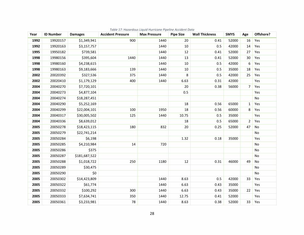
Table 17: Hazardous Liquid Hurricane Pipeline Accident Data Year ID Number Damages Accident Pressure Max Pressure Pipe Size Wall Thickness SMYS Age Offshore?

1992 19920157 $1,349,941 900 1440 20 0.41 52000 16 Yes 1992 19920163 $3,157,757

1440 10 0.5 42000 14 Yes

1995 19950182 $739,581

1440 12 0.41 52000 27 Yes 1998 19980156 $395,604 1440 1440 13 0.41 52000 30 Yes 1998 19980160 $4,238,615

1440 10 0.5 42000 6 Yes

1998 19980163 $9,183,666 139 1440 10 0.5 35000 18 Yes 2002 20020392 $327,536 375 1440 8 0.5 42000 25 Yes 2002 20020410 $1,179,129 400 1440 6.63 0.31 42000

Yes

2004 20040270 $7,720,101

20 0.38 56000 7 Yes 2004 20040273 $4,877,104

0.5

Yes

2004 20040274 $18,287,451

No 2004 20040290 $5,252,169

18 0.56 65000 1 Yes

2004 20040299 $22,004,101 100 1950 18 0.56 60000 8 Yes 2004 20040317 $30,005,502 125 1440 10.75 0.5 35000

Yes

2004 20040336 $8,639,012

18 0.5 65000 2 Yes 2005 20050278 $18,423,115 180 832 20 0.25 52000 47 No 2005 20050279 $22,741,214

No

2005 20050284 $6,198

1.32 0.18 35000

Yes 2005 20050285 $4,210,984 14 720

No

2005 20050286 $375

No 2005 20050287 $181,687,522

No

2005 20050288 $1,018,722 250 1180 12 0.31 46000 49 No 2005 20050289 $30,475

No

2005 20050290 $0

No 2005 20050302 $14,423,809

1440 8.63 0.5 42000 33 Yes

2005 20050322 $61,774

1440 6.63 0.43 35000

Yes 2005 20050332 $100,292 300 1440 6.63 0.43 35000 22 Yes 2005 20050333 $7,634,741 350 1440 12.75 0.41 52000

Yes

2005 20050361 $3,233,981 78 1440 8.63 0.38 52000 33 Yes

29

2005 20060007 $6,980,512 200 1440 12.75 0.41 52000 37 Yes 2005 20060010 $727

2312 18 0.69 42000 9 Yes

2006 20060048 $9

1440 8.63 0.38 52000 34 Yes 2006 20060049 $9

1440 8.63 0.38 52000 34 Yes

2006 20060195 $219,799

835 2

1 No 2006 20060346 $11,163,362 70 1440 12.75 0.56 46000 27 Yes 2007 20070201 $78,992 340 1440 8 0.22 52000

No

2007 20080005 $108,892

250 8 0.28

No 2008 20080211 $566

2160 10 0.5 60000

Yes

2008 20080304 $4,712,779 500 1440 10 0.5 52000 25 Yes 2008 20080305 $3,368 670 2160 20 0.56 60000 13 Yes 2008 20080307 $56,127 50 2183

No

2008 20080308 $7,696 75 1950 24 0.5 65000 12 No 2008 20080313 $22,941 70 1250 24 0.5 70000 4 No 2008 20080324 $56,239 1050 1440 10 0.5 42000

Yes

2008 20080337 $7,857,773

2160 6 0.63 52000 2 Yes 2009 20090235 $11,946,709 750 1440 20 0.41 52000 33 Yes 2010 20100045 $2,422,980 400 1407 18 0.406 52000 42 Yes 2012 20120258 $1,175

No

2012 20120263 $531,048 5 285

4 No 2012 20120281 $497,694

1200

4 Yes

2012 20120344 $37,486

Yes

30

References Chris Landsea. “FAQ E23) What Is the Complete List of Continental U.S. Landfalling.” NOAA: Hurricane

Research Division, June 1, 2017. http://www.aoml.noaa.gov/hrd/tcfaq/E23.html. Cruz, A. M., and E. Krausmann. “Hazardous-Materials Releases from Offshore Oil and Gas Facilities and

Emergency Response Following Hurricanes Katrina and Rita.” Journal of Loss Prevention in the Process Industries 22, no. 1 (January 1, 2009): 59–65. https://doi.org/10.1016/j.jlp.2008.08.007.

Cruz, Ana Maria, and Elisabeth Krausmann. “Vulnerability of the Oil and Gas Sector to Climate Change and Extreme Weather Events.” Climatic Change 121, no. 1 (November 1, 2013): 41–53. https://doi.org/10.1007/s10584-013-0891-4.

Energy Information Administration. “U.S. Energy Mapping System.” Energy Information Administration, 2017. https://www.eia.gov/state/maps.php.

“ExxonMobil Pipeline To Pay $12M Over 2011 Spill Into Yellowstone River - Lexis Legal News.” Lexis Legal News, September 21, 2016. http://www.lexislegalnews.com/articles/11347/exxonmobil-pipeline-to-pay-12m-over-2011-spill-into-yellowstone-river.

Field, Christopher, Vicente Barros, Thomas Stocker, Qin Dahe, David Dokken, Kristie Ebi, Michael Mastrandrea, et al. “Managing the Risks of Extreme Events and Disasters to Advance Climate Change Adaptation.” Cambridge: Intergovernmental Panel on Climate Change (IPCC), 2012. https://www.ipcc.ch/pdf/special-reports/srex/SREX_Full_Report.pdf.

Girgin, S., and E. Krausmann. “Historical Analysis of U.S. Onshore Hazardous Liquid Pipeline Accidents Triggered by Natural Hazards.” Journal of Loss Prevention in the Process Industries 40 (March 2016): 578–90. https://doi.org/10.1016/j.jlp.2016.02.008.

Kishawy, Hossam A., and Hossam A. Gabbar. “Review of Pipeline Integrity Management Practices.” International Journal of Pressure Vessels and Piping 87, no. 7 (July 2010): 373–80. https://doi.org/10.1016/j.ijpvp.2010.04.003.

Kossin, J.P., T. Hall, T. Knutson, K.E. Kunkel, R.J. Trapp, D.E. Waliser, and M.F. Wehner. “Extreme Storms.” In Climate Science Special Report: A Sustained Assessment Activity of the U.S. Global Change Research Program, 375–404. Washington D.C.: U.S. Global Change Research Program, 2017.

Mufson, Steven, and Chris Mooney. “Keystone Pipeline Spills 210,000 Gallons of Oil on Eve of Permitting Decision for TransCanada.” Washington Post, November 16, 2017, sec. Energy and Environment. https://www.washingtonpost.com/news/energy-environment/wp/2017/11/16/keystone-pipeline-spills-210000-gallons-of-oil-on-eve-of-key-permitting-decision/.

Parvizsedghy, L., and T. Zayed. “Developing Failure Age Prediction Model of Hazardous Liquid Pipelines,” June 2015. https://doi.org/10.14288/1.0076416.

Pipeline and Hazardous Materials Safety Administration. “Accident Incident and Mileage Summary Statistics.” phsma.dot.gov, 2017. https://www.phmsa.dot.gov/portal/site/PHMSA/menuitem.7c371785a639f2e55cf2031050248a0c/?vgnextoid=3b6c03347e4d8210VgnVCM1000001ecb7898RCRD&vgnextchannel=3b6c03347e4d8210VgnVCM1000001ecb7898RCRD&vgnextfmt=print.

———. Definitions, 49 CFR 191.3 Electronic Code of Federal Regulations §. Accessed September 4, 2017. https://www.ecfr.gov/cgi-bin/text-idx?SID=1d0466f543b066f6030889bd50b18996&mc=true&node=se49.3.191_13&rgn=div8.

———. “Distribution, Transmission & Gathering, LNG, and Liquid Accident and Incident Data.” Data & Statistics, 2017. http://www.phmsa.dot.gov/pipeline/library/data-stats/distribution-transmission-and-gathering-lng-and-liquid-accident-and-incident-data.

———. “ExxonMobil Silvertip Pipeline Crude Oil Release into the Yellowstone River in Laurel, MT on 7/1/2011.” Homeland Security Digital Library, October 2012. https://www.hsdl.org/?view&did=729780.

31

———. “Hazmat Incident Report Search.” Incident Statistics, 2017. http://www.phmsa.dot.gov/hazmat/library/data-stats/incidents.

———. “Instructions For Form PHMSA F 7000-1 (Rev. 10-2011) Accident Report – Hazardous Liquid Pipeline Systems.” Washington D.C., 2011. https://www.phmsa.dot.gov/sites/phmsa.dot.gov/files/docs/forms/12436/hlaccidentinstructionsphmsa-f-7000-1on-or-after-january-1-2010_0.pdf.

———. “Instructions For Form PHMSA F 7100.2 (Rev. 06-2011) Incident Report – Natural And Other Gas Transmission And Gathering Pipeline Systems.” Washington D.C., 2011. https://www.phmsa.dot.gov/sites/phmsa.dot.gov/files/docs/forms/12616/gtggincidentinstructionsphmsa-f-71002on-or-after-january-1-2010.pdf.

———. Pipeline Safety: Safety of Hazardous Liquid Pipelines; Proposed Rule, 2015–25359 § 195.414 (2015). https://www.regulations.gov/document?D=PHMSA-2010-0229-0041.

———. Reporting Accidents, 49 CFR 195.50 § (2010). https://www.gpo.gov/fdsys/granule/CFR-2010-title49-vol3/CFR-2010-title49-vol3-sec195-50.

———. “Safety-Related Condition Reports (SRCRs),” October 20, 2017. https://www.phmsa.dot.gov/data-and-statistics/pipeline/safety-related-condition-reports-srcrs.

Restrepo, Carlos E., Jeffrey S. Simonoff, and Rae Zimmerman. “Causes, Cost Consequences, and Risk Implications of Accidents in US Hazardous Liquid Pipeline Infrastructure.” International Journal of Critical Infrastructure Protection 2, no. 1–2 (May 2009): 38–50. https://doi.org/10.1016/j.ijcip.2008.09.001.

Senouci, Ahmed, Mohamed Elabbasy, Emad Elwakil, Bassem Abdrabou, and Tarek Zayed. “A Model for Predicting Failure of Oil Pipelines.” Structure and Infrastructure Engineering 10, no. 3 (March 4, 2014): 375–87. https://doi.org/10.1080/15732479.2012.756918.

U.S. Bureau of Economic Analysis. “Gross Domestic Product: Implicit Price Deflator.” FRED, Federal Reserve Bank of St. Louis, 2017. https://fred.stlouisfed.org/series/GDPDEF.

Wang, Yong, Tarek Zayed, and Osama Moselhi. “Prediction Models for Annual Break Rates of Water Mains.” Journal of Performance of Constructed Facilities 23, no. 1 (February 1, 2009): 47–54. https://doi.org/10.1061/(ASCE)0887-3828(2009)23:1(47).