Characteristics of Decision Trees• Decision trees have many appealing properties

– Similar to human decision process, easy to understand– Deal with both discrete and continuous features– Highly flexible hypothesis space, as the # of nodes (or depth)

of the tree increase, decision tree can represent increasingly complex decision boundaries

DT can represent arbitrarily complex decision boundaries

If needed, the tree can keep on growing until all examples are correctly classified! Although it may not be the best idea

How to learn decision trees?

• Possible goal: find a decision tree h that achieves minimum error on training data – Trivially achievable – if use a large enough

tree• Another possibility: find the smallest

decision tree that achieves the minimum training error– NP-hard

Greedy Learning For DTWe will study a top-down, greedy search approach. Instead of trying to optimize the whole tree together, we try to find one test at a time.

Basic idea: (assuming discrete features, relax later)

1. Choose the best attribute to test on at the root of the tree.

2. Create a descendant node for each possible outcome of the test

3. Training examples in training set S are sent to the appropriate descendent node

4. Recursively apply the algorithm at each descendant node to select the best attribute to test using its associated training examples• If all examples in a node belong to the same class, turn it into a

leaf node, label with the majority class

One possible question: is x <0.5?

[8, 0]

?

[13, 15]x < 0.5?

[5, 15]

Continue

This could keep on going, until all examples are correctly classified.

[8, 0]

[13, 15]x < 0.5?

[5, 15]y<0.5?

[4, 0] [1, 15]?

Choosing the best test

25 14

X1

20 8 5 6

T F

25 14

X2

17 3 8 11

T F

Which one is better?

Choosing the best test

25 +

14 -

X1

20 +

8 -

T F

X2

T F

Assuming that we will stop growing the tree after selecting this test. How many mistakes will we make?

5 +

6 -

17 +

3 -

8 +

11 -

25 +

14 -

8+5=13 3+8=11

Choosing the Best test: A General View

S: current set of training examples

Benefit of split = ∑

Total Expected Remaining Uncertainty after the test

25 +

14 -

X1

20 +

8 -

T F

5 +

6 -

S

S1 S2 S1, S2, … Sm: m sets of training examples

M branches, one for each possible outcome of the test

Uncertainty of the class label in S

: The portion of examples in that takes branch

Choosing the best test

25 +

14 -

X1

20 +

8 -

T F

X2

T F

This can be viewed as using the error rate as a measure of the uncertainty.

5 +

6 -

17 +

3 -

8 +

11 -

25 +

14 -

8+5=13 3+8=11

Using error rate as a measure of uncertainty does not always work well

In this example, testing on t did not reduce the error. However, it actually is actually making some “progress” toward a good tree.

26 +

7 -

t

21 +

3 -

T F

5 +

4 - ∗ ∗

A Better Measure: Entropy• Given a set of training examples

– Let denote the label of an example randomly drawn from – If all examples belong to one class, y has zero uncertainty– If takes the positive and negative values with a 50%-50%

chance, we have the highest amount of uncertainty in • In information theory, entropy is the measure of

uncertainty of a random variable

i

k

ii

k

i ii pp

ppyH

1

21

2 log 1log)(

DefinitionLet be a categorical random variable that can take different values: 1, 2, … , ; and for 1,… , . The entropy of , denoted , is defined as

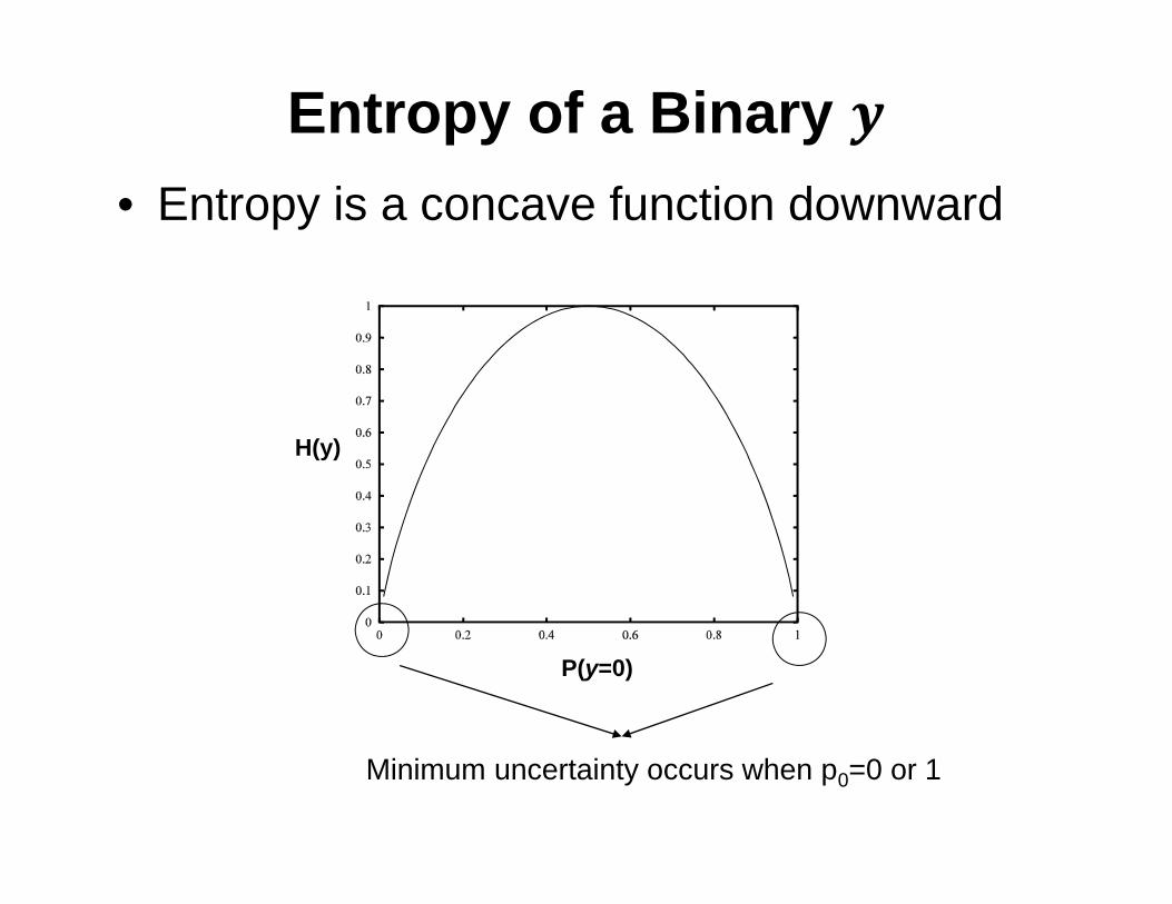
Entropy of a Binary

Minimum uncertainty occurs when p0=0 or 1

• Entropy is a concave function downward

P(y=0)

H(y)

• This measures the Mutual information between and ,• Hence the name information gain

The Information Gain approach:Measuring uncertainty using entropy:

26 +

7 -

t

21 +

3 -

T F

5 +

4 -

2633 log

2633

733 log

733=0.7455

2124 log

2124

324 log

324=0.5436

59 log

59

49 log

49 0.9911

0.74552433 ∗ 0.5436

933 ∗ 0.9911 0.0799

2433

933

Choosing the Best Feature: Summary

Measures of Uncertainty

Error min ,

Entropy log log

Gini Index

Benefit of split = ∑

Total Expected Remaining Uncertainty

after the test

Original uncertainty

t

Example

Selecting the root test using information gain

9 +

5 -

Humidity

3 +

4 -

6 +

1 -

High Normal

. . . .

.

. .

9 +

5 -

Outlook

2 +

3 -

3 +

2 -

sunny Rain

.

4 +

0 -

.

Overcast

.

. . . .

Continue building the tree

9 +

5 -

Outlook

2 +

3 -

3 +

2 -

sunny Rain

??

Overcast

, , … ,

Yes

, , , ,, , ,

, , , ,

Which test should be placed here?

2 +

3 -

, , , ,

Humidity

High Normal

0+

3 -

2 +

0 -

Issues with Multi-nomial Features• Multi-nomial features: more than 2 possible values• Consider two features, one is binary, the other has 100

possible values, which one you expect to have higher information gain?

• Conditional entropy of Y given the 100-valued feature will be low – why?

• This bias will prefer multinomial features to binary featuresMethod 1: To avoid this, we can rescale the information gain:

)()|()(

maxargj

j

j xHxyHyH

Method 2: Test for one value versus all of the othersMethod 3: Group the values into two disjoint sets and test one set against the other

Dealing with Continuous Features• Test against a threshold• How to compute the best threshold j for Xj?

– Sort the examples according to Xj. – Move the threshold from the smallest to the largest

value– Select that gives the best information gain– Trick: only need to compute information gain when

class label changes

• Note that continuous features can be tested for multiple times in a DT

Considering both discrete and continuous features

• If a data set contains both types of features, do we need special handling?

• No, we simply consider all possibly splits in every step of the decision tree building process, and choose the one that gives the highest information gain– This include all possible (meaningful) thresholds

Issue of Over-fitting• Decision tree has a very flexible hypothesis space• As the nodes increase, we can represent arbitrarily

complex decision boundaries• This can lead to over-fitting

t2

t3Possibly just noise, butthe tree is grown largerto capture these examples

Over-fitting

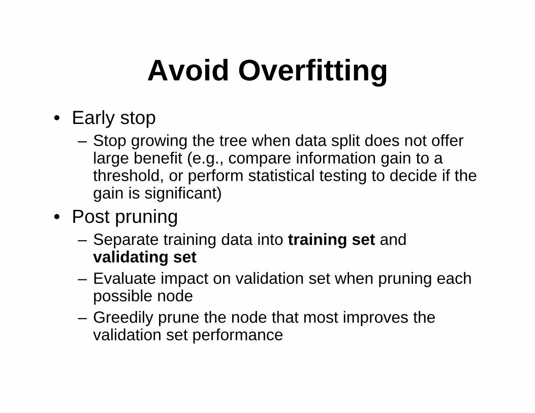
Avoid Overfitting• Early stop

– Stop growing the tree when data split does not offer large benefit (e.g., compare information gain to a threshold, or perform statistical testing to decide if the gain is significant)

• Post pruning– Separate training data into training set and

validating set– Evaluate impact on validation set when pruning each

possible node– Greedily prune the node that most improves the

validation set performance

Effect of Pruning