NASA Technical Memorandum 100046

.

Characteristics of a Separating Confluent Boundary Layer and the Downstream Wake D. Adair W. C. Horne, Ames Research Center, Moffett Field, California

December 1987

.

.

NASA National Aeronautics and Space Administration

Ames Research Center Moffett Field California 94035

https://ntrs.nasa.gov/search.jsp?R=19880004941 2018-07-16T10:04:39+00:00Z

CHARACTERISTICS OF A SEPARATING CONFLUENT BOUNDARY LAYER AND THE DOWNSTREAM WAKE

D. Adair* and W. C. Horne Ames Research Center

SUMMARY

Detailed measurements of pressure and velocity characteristics are presented and analyzed for flow over and downstream of a NACA 4412 airfoil equipped with a NACA 4415 single-slotted flap at high angle of attack and close to maximum lift. The flow remained attached over the main element while a large region of recirculat- ing flow occurred over the aft 61% of the flap. tested at a Mach number of 0.09 and a chord Reynolds number of 1.8 x log in the NASA Ames Research Center 7- by 10-Foot Wind Tunnel. fluctuating velocities were obtained in regions of recirculation and high turbulence intensity using 3-D laser velocimetry. In regions where the flow had a preferred direction and relatively low turbulence intensity, hot-wire anemometry was used. Emphasis was placed on obtaining characteristics in the confluent boundary layer, the region of recirculating flow, and in the downstream wake. Surface pressure measurements were made on the main airfoil, flap, wind tunnel roof and wind tunnel floor. wind tunnel cross section, the wind tunnel floor and ceiling interference should be taken into account when the flow field is calculated.

The airfoil configurati n was

Measurements of mean and

It is thought likely that because the model is large when compared to the

In addition to the presentation of pressure and velocity characteristics, the near-wall results inside the separated region are analyzed as are the relative importance of terms in the momentum and turbulence kinetic energy equations in the confluent separated boundary layer and the recirculating region of the near wake.

*NRC Research Associate.

1

NOMENCLATURE

C main airfoil reference chord, 0.9 m

drag coefficient

lift coefficient (airfoil lift)/(l/2)pU m c

CD

cL 2

cM

cP

c f

H

moment coefficient, around x/c of 0 25, (moment around quarter chord)/(l/2)pUmc

2

2

pressure coefficient, (P - PW)/(1/2)pU W

skin friction coefficient

Shape factor, &*/e

boundary-layer coordinate system over the flap (normal and tan- gential to local surface)

P static pressure

reference chord Reynolds number, pU,c/u Re

u W reference free-stream velocity

mean velocities (in boundary-layer coordinate system and tunnel coordinates downstream)

U-component of turbulence energy 2 <u >

<-uv> Reynolds shear stress

( -uw > Reynolds shear stress

u'/U,,v'/U,,w'/U, Turbulence intensities

2 <v > V-component of turbulence energy

<W2> W-component of turbulence energy

<k2> turbulence kinetic energy

wind tunnel coordinate system (horizontal, vertical, spanwise), with origin at the main airfoil leading edge

(1 angle of attack, deg

2

6P 6

6f

6"

0

V

'e

yPU

< >

Subscripts

e

m

Superscripts

I

pressure parameter

boundary-layer thickness

flap deflection, deg a m

boundary-layer displacement thickness, ( 1 - U/Ue)dz a boundary-layer momentum thickness, ( 1 - U/Ue)dz, or flap normal angle to vertical

fluid density

kinematic viscosity

eddy viscosity

probability of downstream velocity

time average or ensemble average

edge of boundary layer

reference free-stream quantity

perturbation from mean value

I. INTRODUCTION

The multielement wing is essential to generating sufficient lift for modern aircraft during takeoff and landing. is complex, involving significant pressure gradients, nonequilibrium turbulent boundary layers, streamline curvature, and merging asymmetric shear layers. Pres- sure gradients across the wake are significantly larger than those encountered for single-element airfoils. gradients in the streamwise direction, which affects wake-profile development, turbulent transport, and wake entrainment. It also considerably increases the interaction between viscous and inviscid flows in the vicinity of the flap trailing edge.

The flow around such a configuration, however,

The presence of a flap amplifies the adverse pressure

The severe adverse pressure gradients over the aft portion of multielement airfoil arrangements usually flap suction side leading to

cause rapid thickening of the boundary layer on the boundary-layer separation. In addition, the flow field

3

is complicated by the merging of an airfoil wake with a boundary layer of the down- stream element.

Present computational methods can accurately predict the lift (but not drag) of the multielement airfoils at low to moderate angles of attack, providing the flow remains attached. At high angles of attack or when separation occurs, neither lift nor drag can be accurately predicted. An appropriate method for calculating flow over multielement arrangements at high angles of attack has not yet been estab- lished. averaged form of the Navier-Stokes equations and those which solve potential-flow and boundary-layer equations. have been attributed to inadequacies of boundary-layer approximations, especially in accounting for the cross-stream pressure-gradient term, to deficiencies in turbu- lence modeling (ref. l ) , and to the inability to model strong viscous-inviscid interactions successfully (ref. 2) . For a Reynolds-averaged Navier-Stokes approach, two of the major needs are the ability to close the equations with appropriate turbulence model assumptions and the skill to construct computational grids that are compatible with the multielement surface while meeting stringent requirements for smoothness and grid clustering (ref. 3 ) . layers is still a problem for both methods, as turbulence models adequate for the analysis of merging shear layers have not as yet proved sufficiently general. As the adverse pressure gradients become more severe, both techniques face the extra complication of separation. deficiencies, a comprehensive set of measurements will be presented which will be used to analyze the structure of the flow in strong adverse pressure gradients and in evaluating the accuracy of computational methods.

The methods being developed are generally those which solve a Reynolds-

For the latter, the main difficulties in prediction

The calculation of confluent boundary

In order to contribute to a reduction in the foregoing

The present work was preceded by a series of experiments carried out in the NASA Ames 7- by 10-Foot Wind Tunnel. used in this study at a lower angle of attack and with no flow separation is reported in reference 4, and the single-element NACA 4412 airfoil was also tested with trailing-edge separation (ref. 5). Progress has been made elsewhere (refs. 6-8) in the provision of mean and turbulence flow-field data for single- element trailing-edge flows experiencing separation. notable exception of ref. 31, however, is not evident for multielement arrange- ments. In general, data available for multielement airfoils includes static pres- sure measurements, flap optimization, and mean velocity characteristics (refs. 9,lO). Turbulence quantities are not reported to any extent in these studies. Basic studies of a confluent boundary layer and the initial region of boundary-layer separation have been reported in references 11 and 12, respectively.

A test of the multielement airfoil arrangement

Similar progress (with the

In the following sections the surface static pressure and detailed flow-field measurements of mean velocity and components of the Reynolds normal and shear stresses of a turbulent flow in the vicinity of an airfoil equipped with a single slotted flap are reported and analyzed. ent boundary layer over the flap, including the separation region in the vicinity of the flap trailing edge and in the downstream wake. The measurements were made using hot-wire anemometry and a 3-D backscatter laser Doppler anemometer.

The measurements will focus on the conflu-

4

11. EXPERIMENTAL ARRANGEMENT

Wind Tunnel

The test was conducted in the 7- by 10-Foot Wind Tunnel at NASA Ames Research Center, Moffett Field, California. section 4.57 m long a constant height of 2.13 m, and a width which varies linearly from an initial value of 3.05 m to a final value of 3.09 m. There are no turbulence-reducing screens in the wind tunnel circuit, and test section RMS turbu- lence levels u'/U,, v'/U,, and w'/U, respectively, for the chosen test conditions.

The closed-circuit wind tunnel has a working

1

were equal to 0.0025, 0.0085, and 0.0085,

Model

A cross section of the airfoil/flap configuration as installed in the wind tunnel is shown in figure 1 . equipped with a NACA 4415 flap airfoil section. The chord length (c) of the main airfoil is 0.90 m and that of the flap is 0.36 m. flap relative to the main airfoil was specified by the flap gap (FG), the flap overlap (FO), and the flap deflection (tif) as defined in figure 1. For all the velocity characteristics presented in this paper, FG = 0.035 c, FO = 0.028 c, and 6f = 26.8O. throughout the experiment, and references to chord length in the following sections will refer to the main airfoil unless otherwise specified. The coordinate system used in the present work is shown in figure 1. profiles were taken normal to the model surface, whereas in the downstream wake, tunnel coordinates were used. All streamwise distances were referenced to the main airfoil leading edge, and the cross-stream (vertical) origin used for the wake profiles was the flap trailing edge.

The model comprises a NACA 4412 main airfoil section

The geometric location of the

The main airfoil angle of attack ( a ) was set at a value of 8.2"

Upstream of the flap trailing edge

The model wind tunnel installation is shown in figure 2. It has a span of 3.05 m and was mounted horizontally in the test section. This slightly limited the optical access of the laser velocimeter in that part of the flow field immediately adjacent to the trailing edge of the flap when compared with a vertically orientated model. An important advantage is achieved with the horizontal arrangement in that optical flare is reduced when one works close to the surface. The intersections between wall and airfoil sections were sealed using felt pads to eliminate leakage between the pressure and suction flows. Boundary-layer trips were mounted on the suction and pressure surfaces of the main airfoil to ensure uniform flow transition

minimum. A trip was also mounted on the suction side of the flap at an x/c value of 0.01, which was downstream of the flap pressure minimum. Each of the trips had a uniform width of 5.6 mm, a thickness of 0.18 mm, and a sawtooth leading edge.

- across the span at x/c values of 0.025 and 0.10, respectively, from the pressure

Surface static pressures were measured at 66 orifices located on the centerline

Two additional chordwise rows of 56 orifices each on the main airfoil and of the main airfoil and at 42 static pressure orifices located on the centerline of the flap.

5

42 orifices each on the flap were located at 0.35-span and at 0.65-span. In addi- tion, a spanwise row of 22 upper-surface orifices was located at the 0.25-chord of the main airfoil and two spanwise rows of 12 upper-surface orifices each were located at the 0.25-chord and 0.85-chord locations on the flap. at these 350 orifices was measured using eight 48-port scanivalves equipped with 27 kN/m pressure transducers. on magnetic tape with the data reduced to coefficient form. Repeatability in sur- face pressure data proved to be good at all test conditions, with a maximum change in Cp of 0.6% noted between test runs. Integration of the pressure coefficients produced the section lift and moment coefficients

The static pressure

2 The transducer voltages were digitized and recorded

CL and CM.

Test Conditions

All of the data presented in his paper are for a Mach number of 0.09, and a t! chord Reynolds number of

30.0 m/sec monitored using a Pitot-static probe located at 1.4 chord lengths upstream of the main airfoil leading edge and 0.61 m from the wind tunnel floor. The test conditions resulted in a steady flow field with an absence of flow separa- tion on with main airfoil but with boundary-layer separation, over the aft 61% of the flap. Extensive probing of the tunnel wall boundary layers was conducted using tufts and surface oil visualization. be found in those regions. Streamwise flow fences encircling the main airfoil were installed at 0.175-span and 0.825-span locations to shield the central airfoil section from tunnel wall boundary-layer interference. Studies using tufts and surface oil visualization showed the flow to be two-dimensional over the central 65% of the main airfoil's span. flap was also investigated. Over a stalled airfoil it has been shown (ref. 13) that the flow can depart significantly from two-dimensionality. alleviate this using adjustable flow fences on the flap. The fences, shown in figure 2, extended along 30% of chord length on the upper and lower sides of the flap. It was not possible to use fences which ran the full length of the flap since the laser velocimeter required optical access. The final position occupied by the flow fences were 0.39-span and 0.63-span locations. vicinity of the flap trailing edge was found t o extend over the center 20% of flap span.

1.8 x 10 , corresponding to a tunnel velocity (U,) of

No evidence of boundary-layer separation could

The two-dimensionality of the flow over the airfoil

An effort was made to

Two-dimensional flow in the

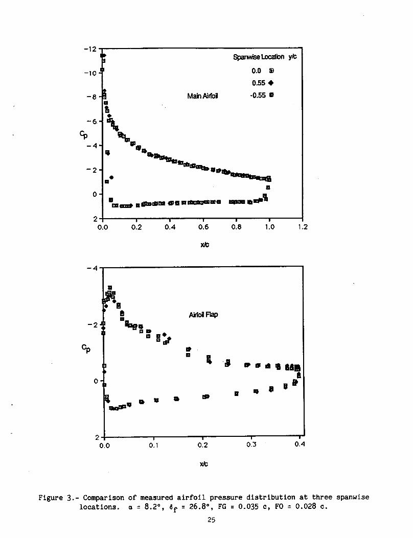
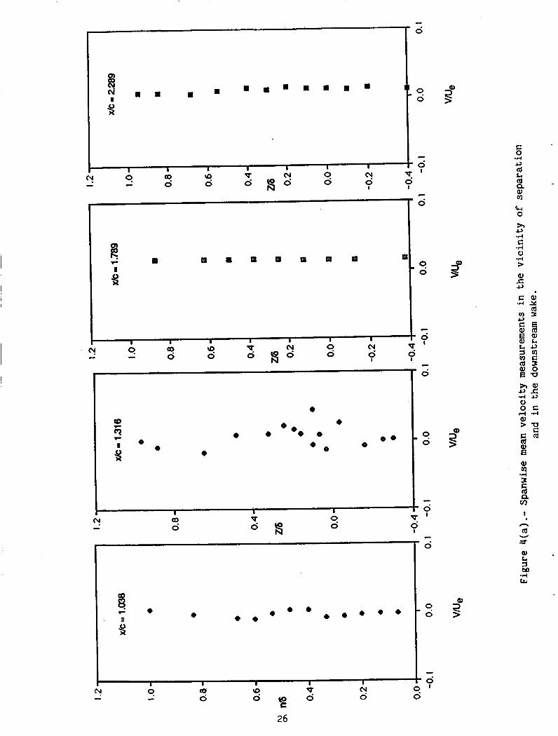
In addition to surface oil and tuft visualization, two-dimensionality of the flow was quantified using pressure and velocity characteristics. profiles along the model centerline and at 482 mm to each side of the centerline are shown in figure 3. The agreement between the three rows of measurements is good except over the initial 30% of flap where it is thought the proximity of the flow fences influenced the measurements at the Y/c = 20.55 locations. Figure 4(a) presents the spanwise mean velocity at the model centerline upstream of and within the separated region and at two locations downstream of the flap trailing edge. Spanwise velocities can be seen t o be generally less than 2% of the free-stream velocity.

Spanwise pressure

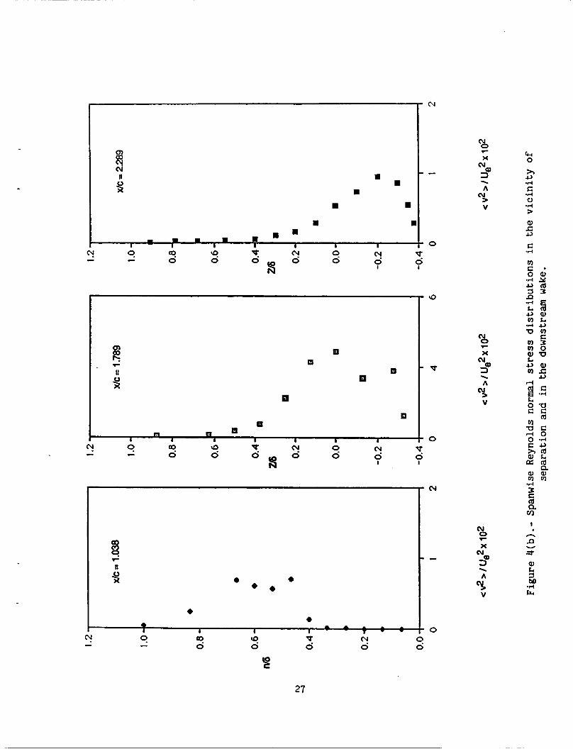
Shown in figure 4(b) are Reynolds stresses measured in the merging shear

Y

6

layers upstream of separation and at two locations in the wake, with the Reynolds shear stress seen to be close to zero in all three profiles (fig. 4(c)).

For the mean velocity and turbulence measurements, profiles were made normal to the main airfoil or flap surfaces upstream of the flap trailing edge as described in table 1 and figure 5. In the downstream wake, profiles were made using wind tunnel coordinates. Table 2 presents the orientation of the profiles relative to the vertical, the development of the boundary-layer edge velocity, and the physical thickness of the boundary layers and free shear layers. The edge velocity for stations 1 through 3 is for the boundary layer on the suction side of the main airfoil, and for stations 4 though 21 it is for the upper edge of the main airfoil wake. Up to and including x/c of 0.989, 6 is the width of the boundary layer on the main airfoil whereas for 1.003 < x/c - < 1.289 it represents the distance from the flap surface to the upper edge of the main airfoil wake. Downstream 6 repres- ents the total physical distance across the wake.

Instrumentation

Pressure characteristics were obtained using surface static pressure taps as reported in an earlier section. diameter of 6.35 mm was used to obtain pressure measurements in the tunnel floor and roof boundary layers, respectively. Vertical surveys using the Pitot-static tube were made at the mid-span location in the plane of the reference Pitot-static probe and at 1.5 chord lengths downstream of the flap trailing edge.

A sting-mounted Pitot-static tube with an outside

Upstream of separation in the region of merging shear layers and for most of the wake, the flow had a preferred direction and comparatively low turbulence'inten- sities. For these reasons it was possible to quantify the velocity characteristics with stationary hot-wire anemometry. U, W, u t , w', and <-uw), and then to obtain V, v', and <-uv>, where U, W, and V indicate streamwise, cross-stream and spanwise velocities, respectively. Straight- wire (DISA 55P10) and cross-wire (DISA 55P64) probes were operated with constant- temperature anemometers (DISA 55M10), and the instantaneous voltages were recorded digitally using an HP 1000 computer prior to analysis. The wires were operated at an overheat ratio of 1.8 and amplifiers were used in the processing of the signal. The bandwidth of the data-acquisition system was 20 kHz. were sampled simultaneously at a rate of 10 samples/sec over a minimum period of 100 sec. DISA hot-wire.ca1ibration rig, with the resulting linearizations stored in the computer.

The sensors were first orientated to measure

The nonlinearized signals

Calibration for both flow velocity and flow angle was performed using a

In regions of reversed flow and high turbulence intensity, a 3-D laser velocim- eter (LV) as described by references 14 and 15 was used. A schematic of the LV system is shown in figure 6 and its position in relation to the model is shown in figure 7. The LV was used to measure the mean velocities U, W, and V and the turbulence quantities u', w', and <-uw>. The system is capable of measuring all three velocity components ( U , W , V ) simultaneously by means of three independent dual- beam channels that operate in backscatter mode. To improve the sampling rate the

7

method of coupling the three channels as reported in reference 14 was modified. The colors violet (476.5 nm) and green (514.5 nm) of an 8-W argon-ion laser were coupled to obtain samples of streamwise and cross-stream components of the mean velocity and the components of the stress tensor. This was followed by a second sample using the blue (488.0 nm) and green colors to obtain the spanwise mean velocity. Vertical and streamwise motions of the focal volume were accomplished by moving the entire LV on a digitally controlled platform. The repeatable positioning of the focal volume was better than 0.5 mm. The support platform was slightly yawed by 2" with respect to tunnel coordinates, and was pitched downwards by 2.75O to allow grazing contact of the focal volume at the semi-span of the wing. the optical table result in slight coupling of all three velocity components. Neglecting the spanwise coupling component led to an estimated decrease in u' , and w' of 0.65, 0.54$, 1.1%, and 0.92%, respectively.

The small pitch and yaw angles of

U, W,

*

An inherently poor signal-to-noise ratio is common to LVs using backscatter. To alleviate the problem it is desirable to minimize the processing bandwidth. However, this can lead to biasing of the incoming data. The present LV incorporates programmable frequency synthesizers that generate mixing frequencies for each chan- nel that can be varied under program control to maintain the mean signal frequency at the center of the bandwidth. resolve directional ambiguity in the measured velocities.

I Frequency shifting by Bragg cells was employed to I

The laser was operated at a power of between 1.75 and 2 W and the effective probe volume length for each channel was found to be 5 mm for the green and violet beams and 2.5 mm for the blue. Each beam had a waist diameter of 0.3 mm. A mineral oil aerosol with a nominal particle diameter of 5 um was introduced into the dif- fuser of the wind tunnel to provide nearly uniform seeding in the test section. general, 1000 samples were taken at each measurement point, although this was increased in difficult areas of the flow.

In

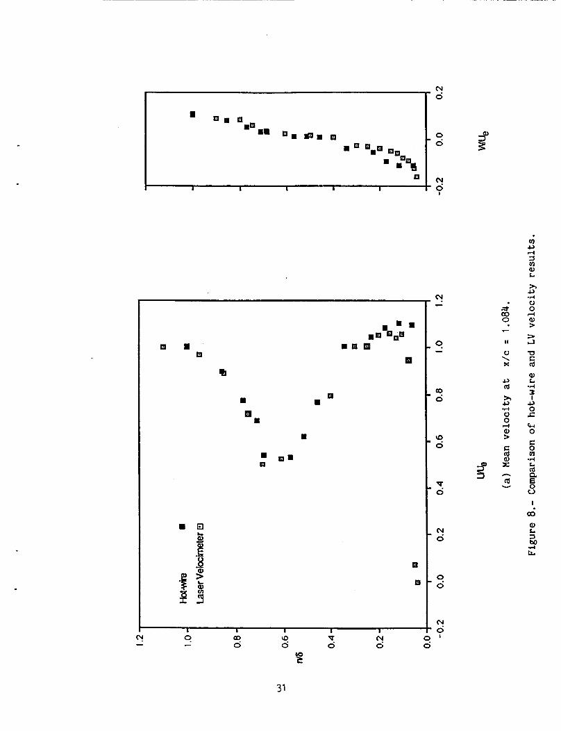
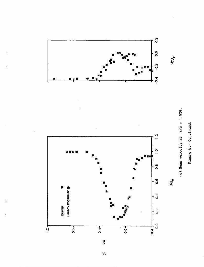
Comparison was made between the hot-wire and LV measuring techniques by compar- ing mean velocity and turbulence characteristics at two streamwise locations, x/c = 1.084 (over the flap) and 1.539 (in the downstream wake). Both locations had regions of intermitt.3t backflow present which affected the hot-wire signal. x/c = 1.084 while at x/c = 1.539 in the wake some backflow occurred in the inner layer. Good agreement was found between the two measuring techniques in the regions where back- flow was not present (fig. 8). The agreement between the two measurement techniques is poor for n/6 < 0.2 for the profile over the flap and for 0.15 > Z/6 > -0.2 for the station in the wake where rectification of the hot-wire signal is evident.

At intermittent boundary layer separation was present close to the surface

111. EXPERIMENTAL RESULTS

The pressure and velocity measurements are presented below for flow both on and downstream of the flap. centerline of the tunnel.

The results presented in this section were obtained on the Particular attention is paid to the regions of the

8

boundary-layer separation, merging shear layers, recirculating flow, and the down- stream wake.

Mean Flow Results-Pressure

Static pressure measured over the main airfoil and flap surfaces at mid-span are presented in figures 9 and 10. Distributions are shown for a range of geo- metries obtained by varying the flap deflection angle and flap gap. Flap overlap

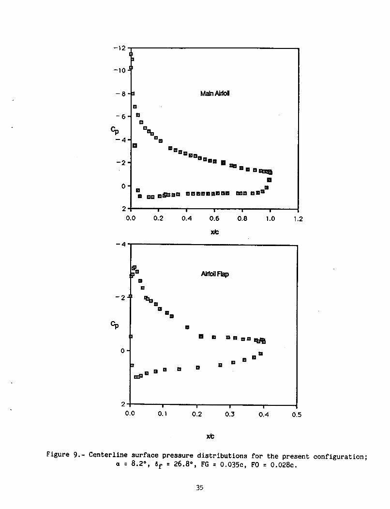
flap gap of 0.035 c (fig. 9) , the existence of separation on the upper flap surface is recognized by the appearance of a constant pressure region extending over 61% of flap chord length. A localized increase in the flap suction is noted at 20% of flap chord, i.e., just downstream of the main airfoil trailing edge. This increase occurred for all the flap settings and was more pronounced when the flap gap was decreased.

was held at a constant 0.028 c for all settings. For the case of 6f of 26.8O and

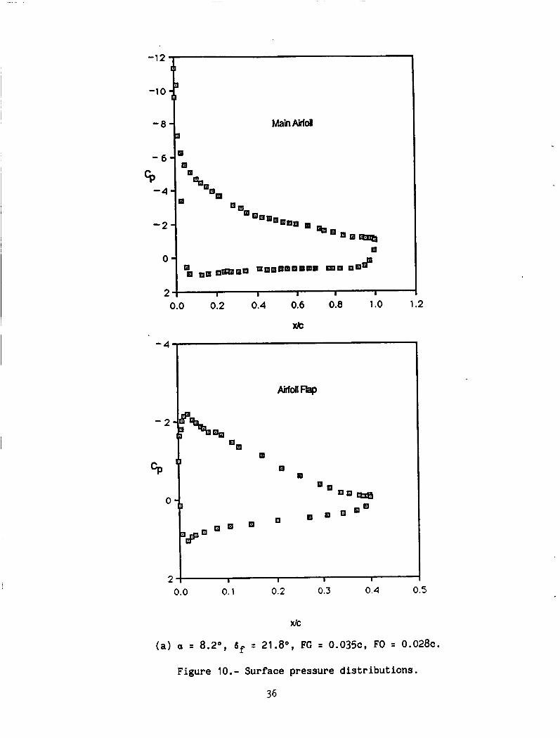
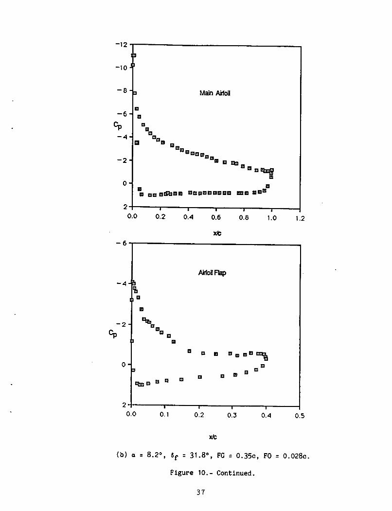
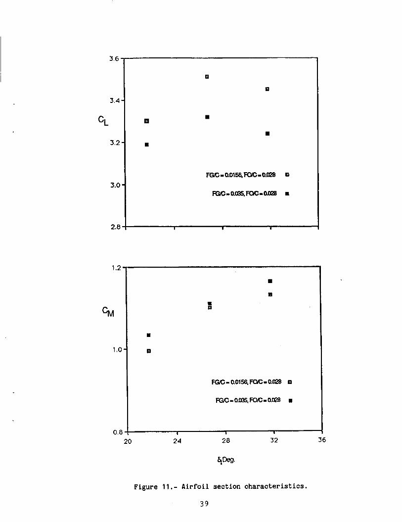
The location of the flap boundary-layer separation could be controlled by both the flap deflection and gap width. a 5" reduction of flap deflection moved the separation point downstream (fig. 10(a)). Increasing the flap deflection by 5" caused the separation to extend over 70% of the flap chord (fig. 10(b)). The effect of flap gap is shown on figure lO(c>. By reducing the gap to 0.015 c and with of the flap chord. Integration of the pressure coefficients produced the section force and moment coefficients CL and CM for the six model settings, the uncor- rected results of which are shown in figure 11. Maximum lift coefficient for a equal to 8.2O is seen to be bounded by the results, but to locate the exact C,

Taking the conditions of figure 9 as a baseline,

The separated region then occupied only the aft 7% of flap chord.

6f = 26.8O, the separation was reduced to 30%

Lmax much finer adjustments of 6f and FG would be required. The values of CL and CM are comparable in magnitude to those reported in references 3 and 16. coefficient, CD, was estimated to be 0.073 for the settings FO = 0.035 c , and FG = 0.028 c . It was estimated by integrating the measured veloc- ity defect 0.5 chord length downstream of the flap trailing edge.

The-drag cSf = 26.8O,

Wind Tunnel Wall Interaction

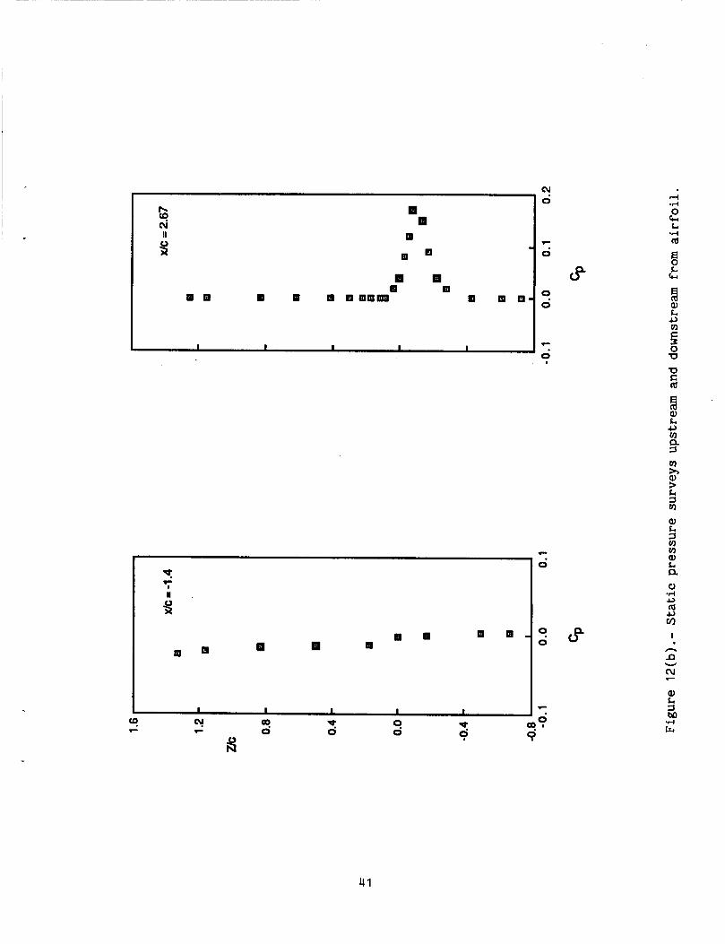
Static pressure measurements were made along the tunnel centerline close to the roof and floor of the test section. These measurements are shown in figure 12 and are for the case fif = 26.8O, FG = 0.035 c, and FO = 0.028 c. The pressure signa- ture on the tunnel walls extended upstream to the plane of the reference Pitot- static probe and downstream into the diffuser. floor boundary layers at the centerline of the tunnel in the plane of the flap trailing edge were obtained to give an indication of the displacement effect of the tunnel wall boundary layers. For the roof boundary layer, 6, 6*, and 8 were found to be 132 mm, 16 mm, and 13 mm, respectively, and for the floor the same quantities were 146 mm, 18 mm, and 14 mm, respectively. Also presented in figure 12 are static pressure measurements taken along vertical traverses. These tranverses were located

Velocity profiles in the roof and

9

at 1.4 chord lengths upstream of the main airfoil leading edge and at 1.5 chord lengths downstream of the flap trailing edge. Total pressure was found to be a constant 601 N/m2 in the plane of the reference Pitot-static tube. measured using a five-tube Pitot probe proved to be within 20.2' from the horizontal.

Flow angularity,

To characterize the effect of tunnel wall interference, calculations with and without tunnel walls were made using the method of reference 17. At the flap deflection angle of 21.B0, when no extensive flow separation occurred, CL and CM were estimated to be decreased by 7% and increased by 4.5%, respectively, when no walls were present. The correction for CL is in close agreement to that found the method for two-dimensional boundary corrections found in reference 18 was used. For the present arrangement, with 6f = 2 6 . B 0 , the method of reference 17 was not appro- priate for correcting lift and pitching moment because of the presence of extensive boundary-layer separation. Thus, because the wall interference effects are expected to be significant and because it is not possible to correct the data reliably for their effects, it is recommended that account should be taken of the presence of wall interference when calculating this flow.

Mean Flow Results-Velocity

The following mean velocity results are for the flap setting 6f = 26.8', FO = 0.035 c , and FG = 0.028 c. tion of the flow domains are shown in figure 13 where is the fraction of LV samples having a positive value of streamwise velocity, 1: Evidence of boundary- layer separation was first noted 228 mm upstream of the flap trailing edge, where a region of intermittent separation, over 4% of flap chord in length, occurred just upstream of boundary-layer detachment. This confirms earlier observations in oil and tuft studies of the location of boundary-layer separation. mittent backflow is seen to envelop the recirculating flow, and negative flow was found to persist to about 180 mm beyond the trailing edge. The maximum height of the fully reversed region was found to be 148 mm normal to the flap surface.

The characteristic boundaries and general organiza- y

A region of inter-

The mean velocity vectors are plotted in figure 14(a); the backflow was rela- tively strong compared to previous studies (refs. 6,8,12). recirculating flow, a thin strip of almost zero velocity existed. Profiles down- stream of the flap indicate the flow developed into an asymmetric wake. The mean flow streamlines in the region of the flap and in the near wake are shown in fig- ure 14(b). The negative mean velocity region is bounded by the zero streamline. In common with the flows of reference 8, the present boundary layer separated under the action of adverse pressure gradients with convex curvature present. The curvature of the streamlines was less than that of the surface. This gave a streamline pat- tern different from that of reference 12, in which streamlines show more curvature near mean streamline detachment when separation was caused by adverse pressure gradient with no surface curvature present.

Close to the top of the

Integral parameters for flow in the vicinity of the flap trailing edge are shown in figure 15. Up to the flap trailing edge, these parameters were obtained by

10

integrating the velocity profiles from the flap surface in a direction normal to the local surface. The integration was terminated at the upper edge of the main airfoil wake. For locations downstream of the trailing edge, the integration was carried out across the entire wake in a vertical direction. The values of the integral quantities are of limited use in that the terms in the cross-stream momentum equa- tion are important in this region and the main airfoil wake has merged with the flap suction-side boundary layer. Large values of 6" and 8 were found in the vicinity of the flap trailing edge, with the maximum found 8% upstream of the flap trailing edge.

Integration of velocity profiles was also performed for the inner flap boundary layer. rapidly before merging with the main airfoil wake. intermittent separation was known to occur, the values of 6" and 0 found by inte- grating across this inner boundary layer were 4.95 mm and 1.60 mm, respectively. This gave a shape factor H of 3.09.

Just upstream of separation the flap boundary layer was found to grow A t 36% of flap chord, where

The skin friction coefficient distributions near the wing trailing edge and on the flap upper surface are shown in figure 16. The skin friction was obtained from Clauser plots. Figure 16(b) indicates mean streamline detachment at 39% of the flap chord (Cf = 0.0). flow visualization.

This is in agreement with the static pressure measurements and

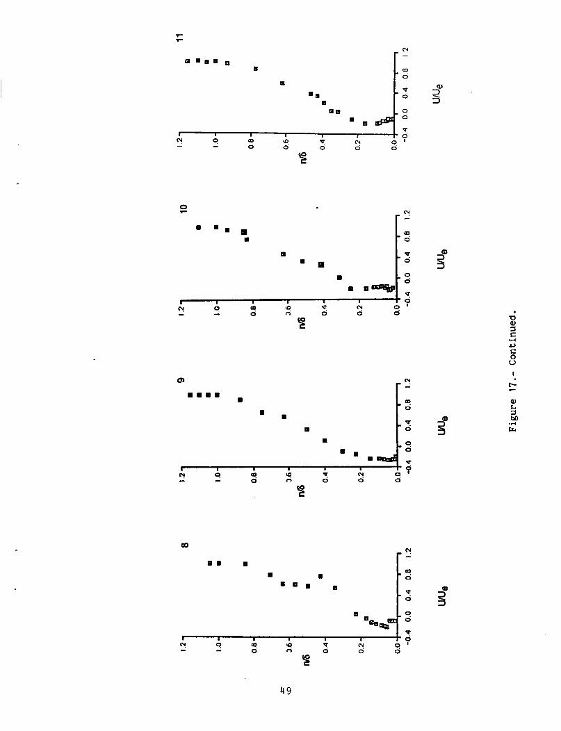
Profiles of streamwise mean velocity are shown in figure 17 for all 21 stations

Just downstream of the main airfoil of table 1. boundary layer in an adverse pressure gradient. trailing edge, the turbulent boundary layer on the flap was found to be extremely thin. At survey station No. 6, the wake of the main airfoil and boundary layer on the upper side of the flap were beginning to merge. of the strong inviscid jet through the slot between main airfoil and flap remained. Backflow, which was first noted close to the surface at station No. 6, strengthened under the influence of the streamwise adverse pressure gradient, to an observed maximum value of 14% of the upper edge velocity at station No. 7. This very strong backflow was also found downstream at stations No. 8 and 9. est recirculating flow was noted at station No. 10, where its value reached 28% of the upper edge velocity. previously for trailing-edge flows and indicates the presence of severe adverse pressure gradients.

The profiles over the main airfoil are consistent with those of a

By station No. 7 only a remnant

The strong-

This is a much stronger backflow than has been reported

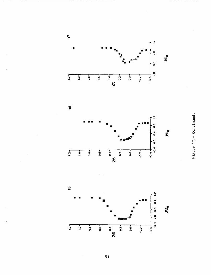
Closure of the wake around the downstream end of the separation bubble occurred because of the interaction of the energetic lower pressure side flow with the sepa- rated shear layer on the suction side. No evidence of a double wake was found downstream of the flap trailing edge, showing the main airfoil wake to have fully merged with the flap wake ahead of this location. had a thickness of 13.5 mm at the trailing edge of the flap. rithmic region which gave a Cf value of 0.004. Values of 6" and 0 for the pressure side boundary layer at the flap trailing edge were found to be 2.53 mm and 1.82 mm. and up t o about

The pressure side boundary layer It had a small loga-

Downstream of the flap trailing edge the wake was seen to be asymmetric x/c = 0.8 the pressure and suction edge velocities were unequal.

11

Further downstream the velocity defect gradually decreased and the shap factor asymptotically approached 1.0.

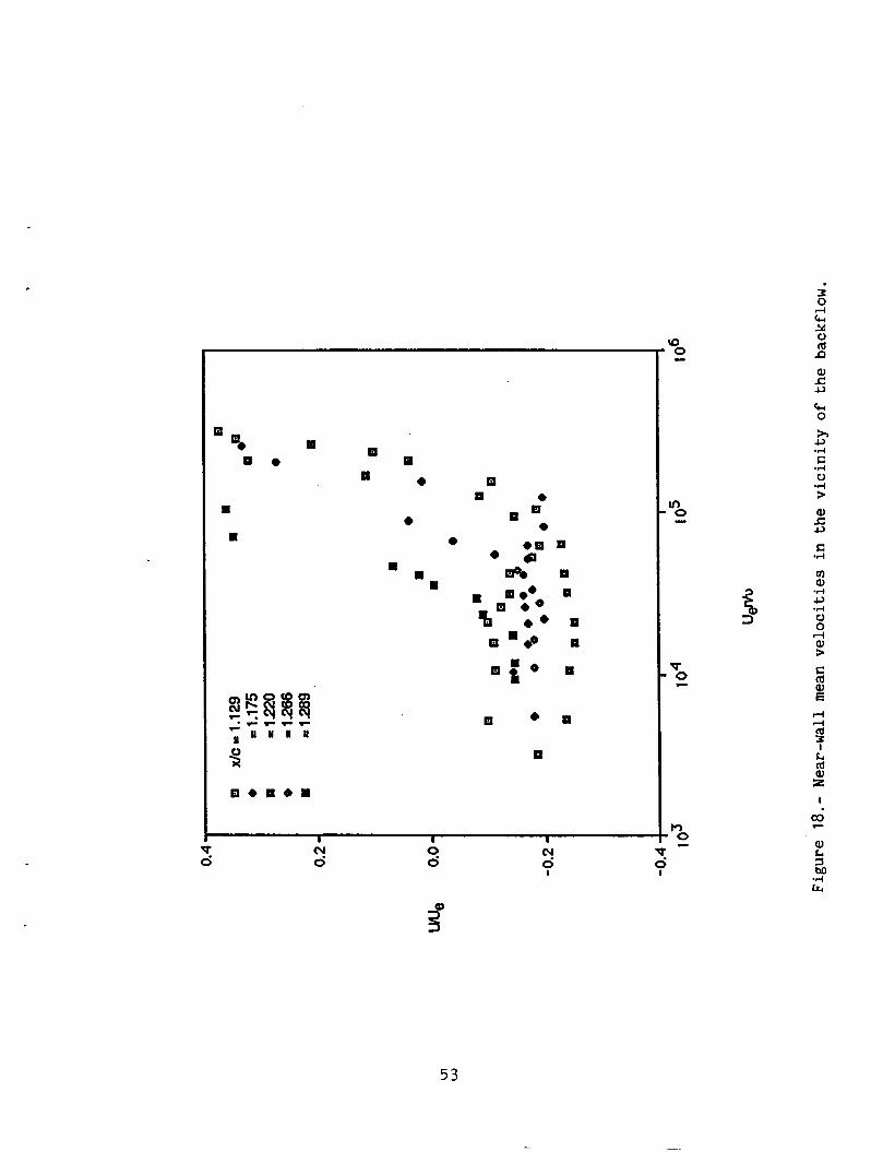
The mean streamwise velocities in the near-wall region of the attached boundary The conventional law-of-the-wall was layer and reversed-flow regions were examined.

found to adequately represent the near-wall flow until just before intermittent separation. After separation there does not appear to be a log-linear region as shown in figure 18.

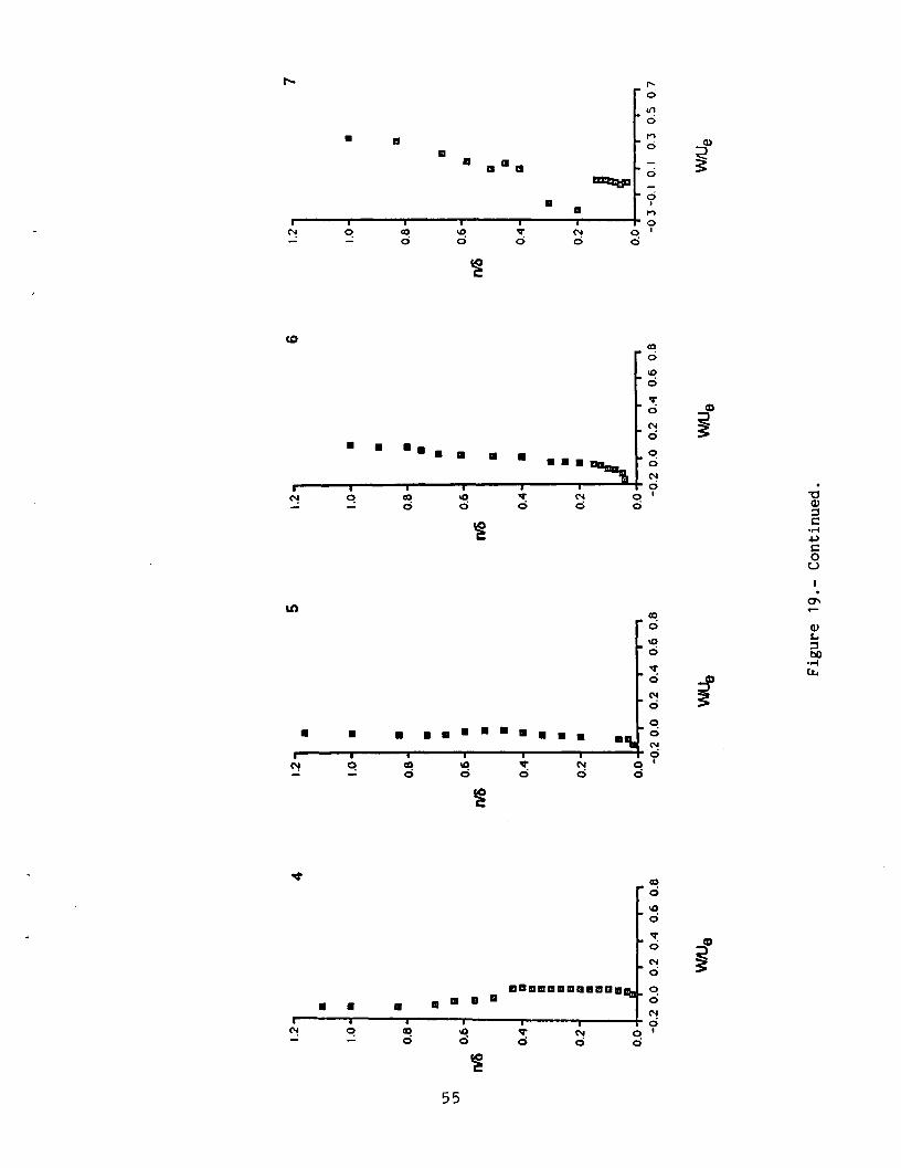
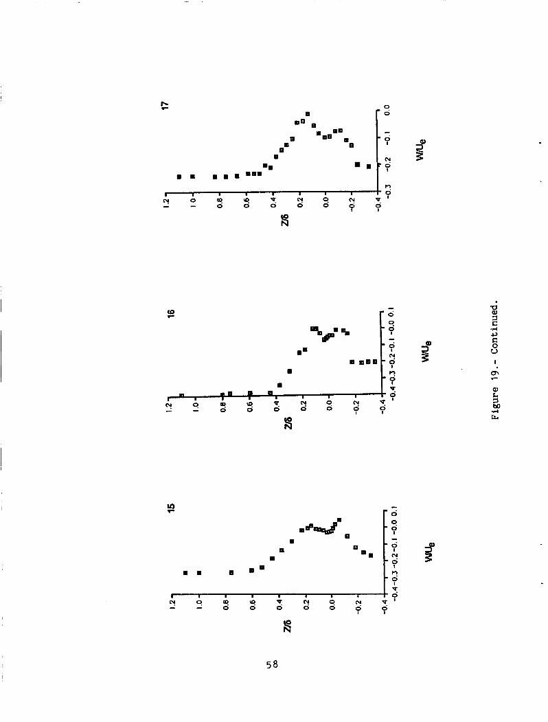
The cross-stream velocity at the 21 stations is presented in figure 19. Gen- erally its value over the main airfoil and initial flap surfaces intended to zero. At station No. 6, close to intermittent separation, flow towards the flap surface of 20% of edge velocity was noted near the surface. Strong variations in cross-stream velocity were found in the wake close to the flap trailing edge and in the vicinity of recirculating flow. For example, at stations No. 12 and 16 cross-stream veloci- ties of up to 30% of free-stream velocity are evident, showing the presence of large cross-stream pressure gradients. This variation tends to diminish with streamwise distance until an almost constant cross-stream velocity profile is noted at x/c of 2.789 (station No. 21).

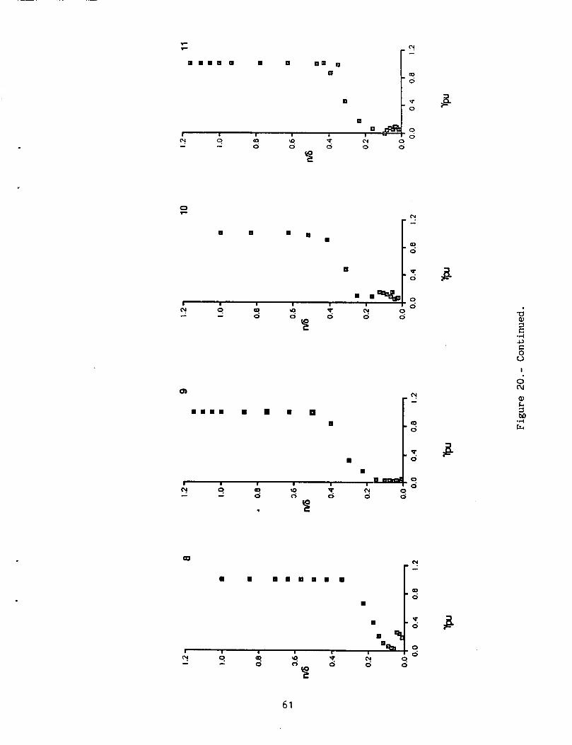
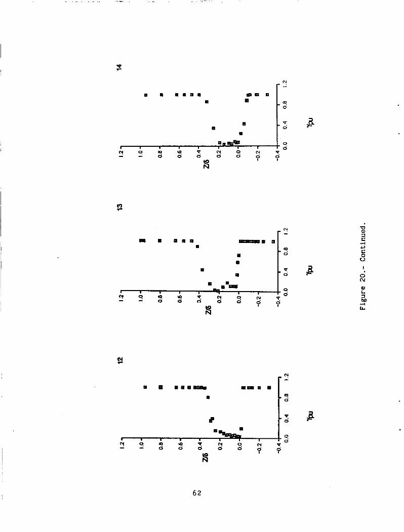
The LV gave information on the probability of downstream flow, ypu in the vicinity of separation. As shown in figure 20, intermittent reversed flow started at 35% (station No. 6) of flap chord and the distance. Also, with downstream distance the instantaneous flow reversals gradually spread cross-stream from the flap surface. In the near wake, it can be seen that

$)I: flap trailing edge. ypu was never found to be zero, indicating no constant, fully reversed flow in any part of the recirculating region, but values as low as 0.02 were found in the vicinity of the flap trailing edge. This is a lower value than was found for stalled, single-element airfoils. At the trailing edge, instan- taneous flow reversals were observed to occur over the inner 42% of the boundary layer, whereas the average mean flow was negative for only 28% of the boundary layer thickness.

ypu values decreased with downstream

of less than 1 was still found at x/c of 0.25 (station No. 16) downstream of

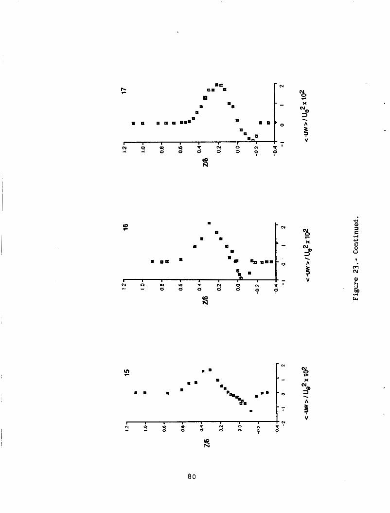
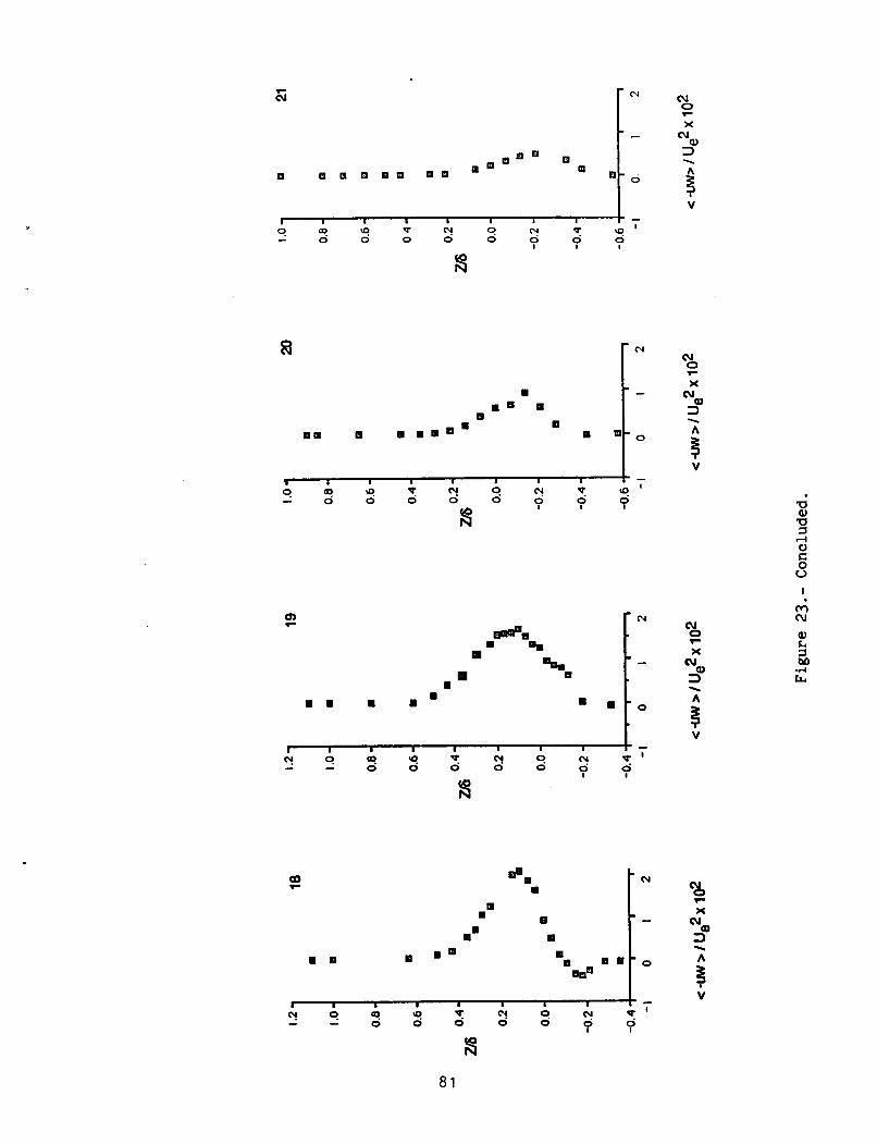
Turbulence Results

The development of Reynolds stresses over the main airfoil and flap suction surfaces and in the downstream wakes are shown in figures 21-23. Comparison of the data obtained at station No. 3 with that obtained at station No. 4 in figures 21 and 22 shows that, initially, there was a significant change in the level of turbu- lence energy near the centerline of the wake as the boundary layer on the upper surface of the wing moved into the near wake and streamwise normal stresses locally increased by 50%. A downstream increase of some 2.6 times in the peak cross-stream normal stresses, as shown by profiles at stations No. 5 and 6 in figure 22, was noted as the shear layer entered a region of increasing adverse pressure gradient, whereas the peak streamwise normal stresses increased only slightly. In the initial regions of jet flow, between the main airfoil and flap, the turbulence was

12

remarkably low. Up to and including station No. 6, the flap boundary layer either cannot be detected or was extremely thin.

The Reynolds shear stress profile (fig. 23) just downstream of the trailing edge of the main element (station No. 4) shows a four-fold increase in peak value compare$ to the profile at station No. 3 . The measured positive peak value of <-uw>/Ue was 0.012 for the wake of the main airfoil compared to the 0.005 reported in reference 4. The negative peak was only about 50% of the value reported in reference 4 at this location. A decline in the Reynolds shear stress is noted near the wall in the wake of the main airfoil in the region of merging shear layers as shown by profiles No. 4-6, and the shear stress goes through zero at station No. 6, further confirming earlier observations that separation first occurs close to this location.

At station No. 7 the flap boundary layer has fully separated and an abrupt change is noted in figures 21 and 22 in the near-wall Reynolds normal stress pro- files. This is consistent with the rapid growth of the separated boundary layer and the disappearance of the low-turbulence jet flow. Downstream of station No. 7 the distributions of streamwise Reynolds normal stresses in the flap suction-side bound- ary layer show the well accepted trends of those in strong adverse pressure gradi- ents, i.e., increasing turbulent stresses with maximum stress points moving away from the walls with streamwise distance. profiles followed this trend in the initial region of the separated boundary layer, but for the increase in peak value and movement away from the wall was minima: and the profiles showed similarity except close to the flap sur- face. Over the region 1.129 < x/c < 1.289 (stations No. 7-11) the maximum values of streamwise and cross-stream-Reynoids normal stresses increased by two and four times respectively because of extra turbulence production and destabilizing curva- ture. The value of the cross-stream Reynolds normal stresses are generally 40% of the streamwise Reynolds normal stresses in the flap trailing-edge region. interesting to note within the recirculating flow and close to the flap surface the appearance of a second maximum in the streamwise normal stress profiles and some of the cross-stream Reynolds normal stress profiles. of a thin but fairly strong reversed boundary layer close to the model surface. No suppression of turbulence in the outer part of the separated boundary layer was indicated by the Reynolds normal stress profiles, and in fact increased turbulence activity in this outer region was noted in profiles No. 10 and 11, causing an equiv- alent increase in Reynolds shear stress. Both cross-stream and streamwise normal stresses peaked at about the same location in the layer, and the cross-stream Reynolds normal stresses show broad maxima, especially in the vicinity of the flap trailing edge, indicating that turbulent diffusion plays an important role here.

The cross-stream Reynolds normal stress

1.220 < x/c < 1.289

It is

This may be due to the presence

Inside the separated region, the Reynolds shear stress gradually develops a double maxima, one close to the surface and the other moving slowly away from the surface with downstream distance. streamwise, and the locations of the Reynolds shear stress zero values seem to cor- respond to that of the minimum in the mean velocity distributions.

Both positive and negative maxima increase

13

In the region just downstream of the flap trailing edge (stations No. 12-16), the Reynolds normal and shear stresses exhibit rapid changes near the wake center- line while changes are gradual towards the outside of the shear layer. It is inter- esting to note the remnant of the near-wall normal stress peak persisting into the

I wake at station No. 12. The profiles show double maxima in the initial Reynolds I normal stress profiles until the end of the recirculating flow region, where the

cross-stream Reynolds normal stresses became single peaked. investigations (refs. 6,19), the streamwise Reynolds normal stresses were slower to decay and it was not until about x/c of 2.039 that the mixing process smooths out the smaller pressure-side peak and a single maximum occurred. Generally, in the near wake the turbulence energy in the pressure-side shear layer increased, whereas on the suction-side layer it remained fairly constant. of 1.789), the streamwise turbulence intensities showed only small variations with streamwise direction, whereas the cross-stream turbulence intensities showed peaks which both increased in magnitude and spread across the layer, showing turbulent diffusion to be dominant as opposed to stabilizing curvature. On the suction side (up to x/c of 7.4271, the streamwise turbulence intensity slightly decayed, whereas the cross-stream turbulence intensity peak remained fairly constant and spread across the shear layer, again showing turbulent diffusion to be present. The location of minimum turbulence intensity in the near wake did not coincide with that of the minimum velocity, indicating a departure from equilibrium.

As found by previous

In the wake (up to x/c

Downstream of the recirculating flow region, the present results are consistent wi h t e mea ure ents f r ferences 19 and 20 and indicate that <u >/U trailing edge the turbulence was found to be essentially isotropic.

$ 9 $ 9 9 5 > <v >/Urn > <w >/Urn. Two chord lengths downstream of the main element's m

In the near wake, the Reynolds shear stress remained fairly constant in the suction-side shear layer, even under the combined influence of adverse pressure gradient and destabilizing streamline curvature. There was a slight increase in its value in the vicinity of intermittent backflow and slightly beyond at about of 1.539 (station No. 16), after which there was a gradual decay. shear stress in the pressure-side shear layer exhibited rapid growth just downstream of the flap trailing edge, then remained constant up to about x/c of 1.539, after which a gradual decay was noted.

x/c The Reynolds

IV. DISCUSSION

The flow just described is now discussed with an emphasis on the relative importance of the terms in the momentum and turbulence kinetic energy equations in the confluent boundary layer and the recirculation region of the near wake. cations for calculation methods will also be discussed.

Impli-

,

~

The calculation of the start of separation in any computational method is important. diction of the onset of separation can be used for the thin boundary layer on the

One question to be addressed is whether standard criteria for the pre-

14

surface of the flap or does the presence of the initially inviscid and later low turbulence jet, and the main airfoil wake affect these criteria. The simple rela- tionship given by reference 21 where

was tested as a necessary criteria just upstream of intermittent separation. measured shape factor showed a discrepancy of 12% when compared to that found by the above equation. Other proposals involve the use of the pressure gradient to predict separation. where

The

For example, reference 22 requires that the parameter Bp > 0.004

Using this criteria, separation was predicted at 34% of flap chord, slightly upstream of known intermittent separation. Because the flow is rapidly changing in this region, the above two results seem to indicate that standard methods of pre- dicting separation can be accurate provided the main airfoil wake has not fully merged with the flap boundary layer.

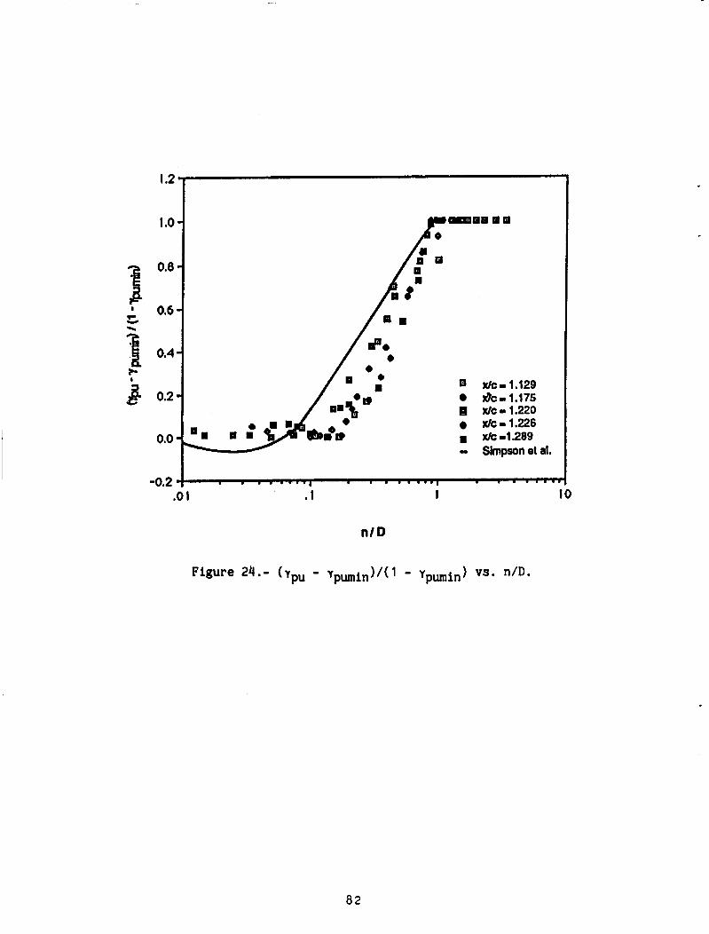
Downstream of intermittent separation, reference 12 shows the existence of

PU - Yp%in)/ similarity in y distributions by normalizing and plotting (y PU

distribution from the wall. ) vs. n/D where D is the distance of the peak in the

PYnin ( 1 - Y u' The present data were compared to a curve which approximately satisfied their data (fig. 24). profiles, but at a different location to that previously found. ily due t o the change in location of the maxima in the u' presence of curvature and/or the contribution to the turbulence field by the main element wake. Similar piots drawn with D being taken as the distance from the wall to the location where peaks are observed in the w' and <-uw> distributions show similar results.

Similarity can be seen in the present This may be primar-

distribution by the

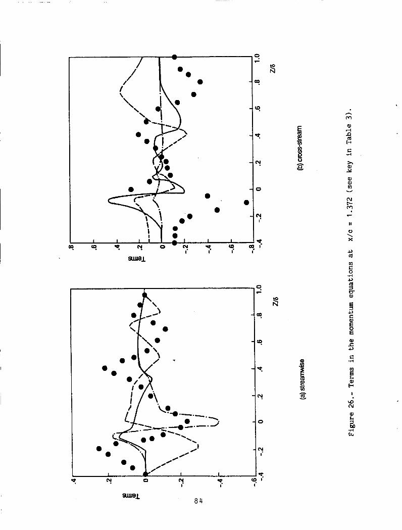
The momentum and energy balance equations were examined in light of the experi- The locations examined included regions in the separated flow, mental measurements.

one in the separated boundary layer and the other downstream in the recirculating flow of the near wake. The momentum equations in two dimensions are

2 a<w > - 1 ap ~<-uw> u - + w g = - - - aw aw + ax o az ax az with the terms on the left-hand side being inertia or convective terms and those on the right-hand side being pressure gradient, the Reynolds shearing-stress gradient, and the Reynolds normal-stress gradient, respectively. For both momentum equations the viscous terms were neglected as they proved to be much smaller than the above

15

terms, and the symbols used for each of the terms in figures 25-27 are shown in table 3.

The cross-stream pressure gradient, as shown in figure 25(b) is important in the vicinity of the trailing edge when it is compared to the corresponding stream- wise pressure gradient (fig. 25(a)). Both terms are generally an order of magnitude larger than those reported for single-element airfoils (refs. 6-8). This suggests that the interaction between the viscous separated boundary layer and the inviscid flow above was strong and that the possibility of successfully applying simple approximations for aP/ay in the boundary layer equations is remote. Just in front of the trailing edge and in the region of separated flow, over the inner 35% of the layer, the shear and normal stress components became dominant and tended to balance the pressure term with convection tending to zero. In the outer region of the layer, convection became the dominant term. In the recirculating flow of the down- stream wake, also shown in figure 26, the shear normal stress gradient terms were again dominant and balanced the streamwise pressure gradient.

For the normal momentum equation, the terms of which are shown in figures 25(b)

The Reynolds normal stress term played a large role in the recirculating and 26(b), the pressure gradient was large and exhibited a large variation across the layer. flow close to the flap wall, as also found by reference 12, and the shear term was less prominent. Around the periphery of the recirculation region, the important quantity was found to be the normal stress term and, to a lesser extent, the convec- tion term.

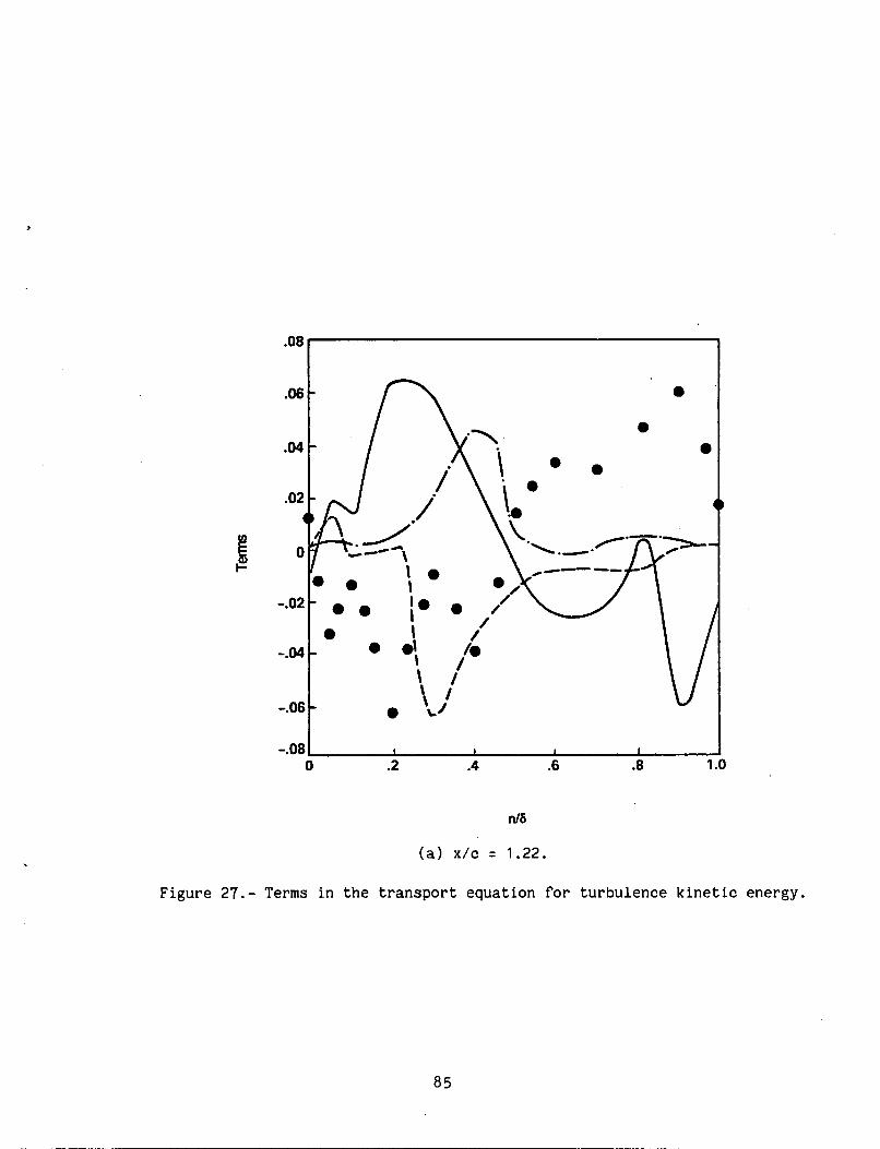
The turbulence energy equation is

( 4 ) -- U a<k2> + - - = - - W a<k2> 2 ax 2 az az az a v (i + $1 - <uw> - au - (<u 2 > - <w 2 > ) au + E

where the terms on the left-hand side are advection and on the right-hand side are turbulent diffusion, turbulent-shear-stress production turbulent-normal-stress foundation, and dissipation, respectively. The turbulence energy equation compo- nents for the present flow are shown for flow over the flap surface in the vicinity of the trailing edge and in the downstream near wake. Dissipation was not measured and appears in the imbalance of figure 27. In the region of recirculating flow over the surface, all three terms-advection, shear production, and normal stress produc- tion-show large variations in the lower 50% of the layer. This would indicate that turbulence energy reaches the backflow region by a combination of turbulence diffu- sion and, to a lesser extent, by convection. In the downstream wake the,shear production term is dominant in the backflow region, whereas normal stress production is evident in the pressure side shear layer. In the upper suction-side layer, advection and shear production are the dominant terms.

The distribution of the shear stress correlation coefficient is shown in fig- ure 28 at several x/c locations. The correlation coefficient is a measure of the extent of the relationship between the instantaneous u' and w' fluctuations. Some similarity was found in the profiles, especially close to the flap trailing edge. Values found in the outer region of the layer were comparable to those found in the

16

fully separated boundary layer of reference 12. close to the model surface.

High negative correlation was noted

Eddy viscosity distributions are shown in figure 29 for five locations in the separated boundary layer; one with intermittent flow reversal present and the others in the separated boundary layer. The minimum noted in the profile at x/c of 1.084 is due to the presence of the low-turbulence jet, and in the separated region v, was defined everywhere except where aU/an = 0. Some similarity was noted in the profiles except in those close to the flap wall. In the outer layer (n/6 > 0.4), the present results show good agreement with those of reference 22, which were measured in adverse pressure gradient equilibrium boundary layers (especially for the flow denoted by the similarity exponent The regression function describing the flow labeled as a = -0.225 ary for the present results. The eddy viscosity derived from the measurements in the present flow are high compared with reference 12, which reported driven down in the presence of separation. The profile at x/c of 1.084 shows good agreement in the inner region of the boundary layer compared with profiles measured in reference 23 and with the eddy viscosity model proposed in reference 24. profiles downstream, however, eddy viscosity models are physically meaningless near the wall as the value tends to infinity.

1

a = -0.15). could be thought of as the upper bound-

ve to be

For

The Prandtl mixing length does not seem to be helpful inside the recirculating region as its use requires taking the square root of a negative term. the modulus of this term was used, similar remarks can be made about the mixing- length profiles as were made for the eddy viscosity inside the separated boundary layer.

However, if

V. CONCLUDING REMARKS

Measurements of the mean values of pressure and velocity have been presented for the flow over and in the downstream wake of a single-slotted airfoil/flap combi- nation. the separation. logarithmic law-of-the-wall in the region approaching separation, but not in the recirculating region. In the vicinity of separation, there is a notable increase in the Reynolds shear stress. The distributions of Reynolds stresses are complex in the very near wake and are affected by streamline curvature and the presence of a significant layer of turbulence. lence field is dominated by shear layers encompassing the separated region. The cross-stream gradient is important in the vicinity of the flap trailing edge and simple approximations for the cross-stream momentum equation do not seem possible. Simple turbulence models are not helpful within the recirculating flow region.

The results indicate rapid'growth of the boundary layer in the vicinity of The mean velocity profiles in the near-wall region agree with the

In the vicinity of the trailing edge, the turbu-

It should be noted that the model was relatively large when compared to the wind tunnel cross section. Thus, it is recommended that the effects of wind tunnel wall interference be included when the flow field is calculated.

17

REFERENCES

1. Spaid, F. W.; and Hakkinen, R. J.: On the Boundary Layer Displacement Effect Near the Trailing-Edge of an Aft-Loaded Aerofoil. J. Appl. Math. Phys., vol. 28, 1977, p. 941.

2. Melnik, R. E.; and Crossman, B.: On the Turbulent Viscous-Inviscid Interaction at a Wedge Shaped Trailing-Edge. Symposium on Numerical and Physical Aspects of Aerodynamic Flows, Springer Verlag, 1981.

3. Braden, J . A.; Whipkey, R. R.; Jones, G . S.; and Lilley, D. E.: Experimental Study of the Separating Confluent Boundary-Layer. NASA CR-3655, 1983.

4. Olson, L. E.; and Orloff, K. L.: On the Structure of Turbulent Wakes and Merging Shear Layers of Multielement Airfoils. AIAA Paper 81-1238, June 1981.

5. Wadcock, A. J.: Investigation of Low-Speed Turbulent Separated Flow Around Airfoils. NASA CR 177450, 1987.

6. Nakayama, A.: Measurements of Attached and Separated Turbulent Flows in t h e Trailing-Edge Regions of Airfoils. Second Symposium at the Calif. State Univ., Long Beach, Jan. 1983.

7. Young, W. H.; Meyers, J. F.; and Hoad, D. R.: A Laser Velocimeter Flow Survey above a Stalled Wing. NASA TP 1266, 1978.

8. Adair, D.: Characteristics of a Trailing Flap Flow with Small Separation. Expts. in Fluids, vol. 5, 1987, pp. 114-128.

9. Foster, D. N.; Irwin, H. P.; and Williams, B. R.: The Two Dimensional Flow Around a Slotted Flap. Farnborough, England, Sept. 1970.

RAE Tech Report 70164, Royal Aircraft Establishment,

10. Olson, L. E.; McGowan, P. R.; and Guest, C. J.: Leading-Edge Slat Optimization for Maximum Airfoil Lift. NASA TM 78566, 1979.

11. Pot, P. J.: Measurements in a 2-D Wake and in a 2-D Wake Merging into a Boundary Layer. NLR Report TR-79063U, National Aerospace Laboratory, The Netherlands, 1979.

12. Simpson, R. L.; Chew, Y. T.; and Shivaprasad, B. C.: The Structure of a Separating Boundary Layer, Parts 1-3. J. Fluid Mech., vol. 113, 1981, pp. 23-90.

13. Winklemann, A. E.: Flow Field Surveys of Separated Flow on a Rectangular Planform Wing. AIAA 19th Aerospace Sciences Meeting, St. Louis, MO, Jan. 1981.

18

14. Orloff, K. L.; Snyder, P. K.; and Reinath, M.S.: Laser Velocimetry in the Low- Speed Wind Tunnels at Ames Research Center. NASA TM 85885, 1984.

15. Snyder, P. K.; Orloff, K. L.; and Reinath, M. S.: Reduction of Flow- Measurements Uncertainties in Laser Velocimeters with Nonorthogonal Channels. AIAA J., vol. 22, no. 8, 1984, pp. 1115-1124.

16. Ljungstrom, B.: Wind Tunnel High Lift Optimization of a Multiple Element Airfoil. FFA Tech. Note AU-778, The Aeronautical Research Institute of Sweden, 1976.

17. Maskew, B.: Program VSAERO, A Computer Program for Calculating the Nonlinear Aerodynamic Characteristics of Arbitrary Configurations. 1982.

NASA CR-166476,

18. Rae, W. H.; and Pope, A.: Low-Speed Wind Tunnel Testing. Wiley, 1984.

19. Hah, C.; and Lakshminarayana, B: Measurement and Prediction of Mean Velocity and Turbulence Structure in the Near Wake of an Airfoil. J. Fluid Mech., V O ~ . 115, 1982, pp. 251-282.

20. Chevray, R.; and Kovasznay, L. S. C.: Turbulence Measurements in the Wake of a Thin Flat Plate. AIAA J., vol. 7, no. 8, 1969, pp. 1641-1643.

21. Sandborn, V. A.; and Kline, S. J.: Flow Models in Boundary-Layer Stall Inception. ASME (J. Basic Eng. ), vol. 83, no. 3, 1961 , pp. 317-327.

22. Alber, I. E.: Similar Solutions of a Family of Separated Turbulent Boundary Layers. AIAA Paper 71-203, Jan. 1971.

23. Bradshaw, P.: The Turbulence Structure of Equilibrium Boundary Layers. J. Fluid Mech., v o l . 29, no. 4, 1967, pp. 625-645.

24. Cebeci, T.; and Smith, A. M. 0.: Momentum Transfer in Boundary Layers. Hemisphere, 1974.

19

TABLE 1.- LOCATION AND ORIENTATION OF SHEAR-LAYER MEASURING STATIONS

Station x/c Type of shear layer Orientation of survey line no.

1 0.495 2 0.742 3 0.989 4 1.003 5 1.038 6 1.084

7 1.129 a 1.175 9 1.220

10 1.266 11 1.289 12 1.316 13 1.372 14 1.427 15 1.483 16 1.539 17 1.622 18 1.789 19 2.039 20 2.289 21 2.789

Boundary layer Boundary layer Boundary layer Wake Wake and boundary layer Confluent boundary layer

Separated boundary layer Separated boundary layer Separated boundary layer Separated boundary layer Separated boundary layer Wake with recirculating flow Wake with recirculating flow Wake with recirculating flow Wake with recirculating flow Wake with intermittent backflow Wake Wake Wake Wake Wake

with intermittent separation

Normal to airfoil surface Normal to airfoil surface Normal to airfoil surface Normal to flap surface Normal to flap surface Normal to flap surface

Normal t o flap surface Normal to flap surface Normal to flap surface Normal t o flap surface Normal to flap surface Tunnel coordinates Tunnel coordinates Tunnel coordinates Tunnel coordinates Tunnel coordinates Tunnel coordinates Tunnel coordinates Tunnel coordinates Tunnel coordinates Tunnel coordinates

20

I TABLE 2.- FREE-STREAM MAIN VELOCITY AND SHEAR-LAYER THICKNESS ~ ~~~

SUCTION-SIDE SURFACE

'e 9 Station x/c

no. m/sec

.. 1 2 3 4 5 6 7 8 9

10 11

0.495 0.742 0.989 1.003 1.038 1.084 1.129 1.175 1.220 1.266 1.289

49.56 43.94 38.00 37.40 36.86 36.50 34.71 32.52 31.20 31.12 31 .OO

20 25 38 76 82 95

145 178 204 240 310

13 17 23 13 19 33 38 41.8 48 48.7 49.0

WAKE

&O. 995 S t a t ion x/c ue (upper) , Ue (lower), no. m/sec m/sec mm

12 13 14 15 16 17 18 19 20 21

1.316 1.372 1.427 1.483 1.539 1.622 1.789 2.039 2.289 2.789

33.09 31.60 31.10 31 .OO 30.98 30.84 30.79 30.75 30.00 29.96

31.70 30.29 28.80 27.52 27.76 28.50 30.94 30.38 29 98 29.83

310 312 320 330 335 343 362 38 1 358 355

21

TABLE 3.- TERMS IN THE MOMENTUM AND TURBULENCE KINETIC ENERGY TRANSPORT EQUATIONS

MOMENTUM TRANSPORT

S treamw i se Symbola

Cross-Stream

-.- 0

-.- 0

TURBULENCE KINETIC ENERGY TRANSPORT

a < k L > + < w > - 3 a < k L > (6*/U,) < u > - a x az 3 2 2 a < u > (6*/U,) < u > - < w > - a x

Imba lance

aSee f i g u r e s 2 5 , 26, and 27.

22

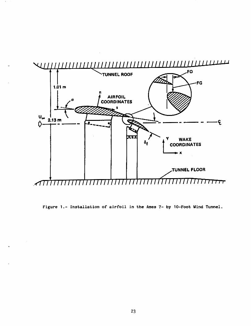
Figure 1.- Installation of airfoil in the Ames 7- by 10-Foot Wind Tunnel.

23

QTOGRAPH ORIGTNAE PAGE IS OF POOR QUALITY

Figure 2.- Model installation in the Ames 7- by 10-Foot Wind Tunnel.

24

-1 2 SpanwiseLOcalii yk

-10

- a

- 6, cp

- 4

- 2 I LI.

0.0 %I

0.55 + Main Airfoil -0.55 0

0.0 0.2 0.4 0.6 0.8 1 .o 1.2

xk

-4k

- 2

CP

0

Z ! I I 1 I 0.0 0.1 0.2 0.3 0.4

xk

Figure 3.- Comparison of measured airfoil pressure distribution at three spanwise locations. a = 8.2O, bf = 26.8O, FG = 0.035 c, FO = 0.028 c.

25

0

8 rn

4 v

I I I I I I I

CI

0

- 8

c

9 c

. -

0

. . i . I I I I O I

c\! c 2 x s 8 $ '

8 r . .

c

0

9 0

- ' Q

cr

(d a W u)

GI 0

2

I n (d v

a, L

.d b

sl

m m

m I

m m I m . I I

I I I I I I m

2s l-

0

9

m a

B

Q

X

%

A

'u> V

0

0 4 O 4

9 c

CJ c

..

cu> V

V

0

9 0

Y 0

a, 5 C 4

I

P a

h

U

a, t

27

x

I I

Q

I I I I I I I

2 x 2 8 n! ? $ ' aD d 9

c n! c

8

9: 0

2

9 0

2

0

0 0 0

0 0 0 0 0 . 0

I I I I I I I

9 - 2 2 x 2 8 h! c

9: 0

2

8

2

X

\

A

5 V

% r X

V

X

\

A

9 V

i I

. I - if ? * t-* JtIC

11 14

1 I 1s

EXPERIMENTAL PROFILES HOT-WIRE LDV

Figure 5.- Orientation and location of velocity profiles.

a i

Figure 6.- 3-D LV.

29

Figure 7.- 3-D LV in relation to wind tunnel and model.

I I I I I I I ? rn I ?

rn

I . . e.

El

rn . .

Q

.B

CJ 0 8 '

I

co

m m Q m w

m m

m Q

Q

cv z X

\

A

V

I I I I I ' P

rn

EI

n m

cv

c

0

M

n P U

V

I .= a . . = m

m I I I x m m l fl .a

.

I

a . n u W

m

ann P

I

e

=. I p m

Ip El'

Ip

e El m m

H Q " 8

b W

El . .=El .- P

I *. * . I I

El

lir

Q -? 6 8 0 \

8 34

M

CJ

c

0

- I

c;J

P

M

cv

c

0

P

M

CJ

-

0

X

3 \ A

V

m cr) L n

X

$ V

3 L 3 b

n

n U W

X

3 \

A

V *!

-12

-1 0

- 8

-6

cp - 4

-2

0

2

1 I

Main Airfoil

0.0 0.2 0.4 0.6 0.8 1 .o 1.2

-41 - 2

cp

0

ID

e

Airfoil Flap

a

0.0 0.1 0.2 0.3 0.4 0.5

Figure 9.- Centerline surface pressure distributions for the present configuration; a = 8.2O, 6f = 26.8', FG = O.O35c, FO = 0.028~.

35

-1 2

- 8

- 6

cp Q

- 2 -'i El 45.0

Main Airid

I El

2 : I I I I I

0.0 0.2 0.4 0.6 0.8 1 .o 1.2

0

rn GJ

0.0 0.1 0.2 0.3 0.4 0.5

xlc

(a) a = 8.20, df = 21.8O, FG = 0.0352, FO = 0.028~.

Figure 10.- Surface pressure distributions.

36

-1 2

-1 0

- 8

-6

CP

-2 -41 Main Moil

El El El

Elm e

2 ! I I I I I

XlC

(b) a = 8 . 2 O , 6f = 31.8", FC = 0.35c, FO z 0.028~.

Figure 10.- Continued.

3 7

- 12

-1 0

- 8

- 6

cp - 4

- 2

0

c A

I

s m m

Main Airloa

0.0 0.2 0.4 0.6 0.8 1 .o 1.2

-4b Airfoil Flap

0.0 0.1 0.2 0.3 0.4 0.5

XlC

( c ) a = 8 . 2 O , 6f = 26.8O, FG = O.O156c, FO = 0 .028~ .

Figure 10.- Concluded.

3.6

3.4

CL

3.2

3.0

2.8

1.2.

CM

1.0,

0.8

El

c1

El

20 24 28 32 36

Slm.

Figure 11.- Airfoil section characteristics.

39

-1 .s

-1 .o

CP

-0.5

0.0

m

H

H

Rad

m /

Q

s 13

Fbor = \

m

xk

0.5

Figure 12(a).- Tunnel wall pressure measurements.

40

rn I o m

e 0

- 0

P 9 0

- 0

9 p 0

0 cu t

E

cu 2

0 .#-I c, ld & r/l I

h

n U

4 1

1 I

-- ------- , - - -______-- , - - - - - -

POTENTIAL FLOW r I

PHYSICAL EDGE OF SHEARLAYER

---- ---

POTENTIAL FLOW

I

I

I I

I

Figure 13.- Flow domains in the v i c in i ty o f the a i r f o i l flap tra i l ing edge.

42

I

1 I I .

I I I I I I I I I I I I I I I

I I I I I I I I I I I I I I I 1

Figure 14(b).- Streamlines in the vicinity of recirculation.

4 3

250

200

tf (m)

1 so

100

L.k.1

so

E

n

GI flap boundary-layer and aHo1 wake aHoilandflapwake8 .

e

B . mo

Ip T.E.

0

e

0 I

2 3

lvc

Figure 15(a).- Integral parameters of mean-flow development.

44

50

40-

e (fm

30 -

2 0 -

IO-

LE.

I&

Figure 15(b).- Integral parameters of mean-flow development.

E flap boundary-layer and airfoil wake 4 airfoil and flap wakes

4 .

4 + 4 +

4

+

4

E

l a m

T.E.

45

0.4 0.6 0.8 1 .o

X/c

(a) On the main a i r fo i l .

1 .o 1.1 1.2 1.3

xlc

(b) On the a ir fo i l flap.

Figure 16.- Distribution of s k i n friction.

46

rn rn a

0 c, L a, Ccl a, L

c 0 .r(

Ccl 0

. . L c, v1 ..-I ca I

tc c

47

rc)

8

m a 0

I I I I I I ' 0 9 r? - 9 2 2 x 2 0

C 0 L)

L zl

" 8 8

B 8

8

0

' 8

m m z

t I I I I I

@!

.=. 0: P

@! 9 x 0 0 0 0 s

0 9 - -

QD

8 8 E

I

pc c

49

d,

. -

O m . 0

r! - [; 0

9 0

P. 0 ' 8

8 .

I I

m 8 t a .. L) '..

a a, 5 c c 0 u I

t- c

E

50

8

8 8 . 0 E

I I

a m 0 0

m

ru

9 0

0 s g I 8

I I

51

cu

" c

2 t B

m am.,

I

tc 7

5 2

3 0

4 0

4

PI E

El CI

0

13

ro 0 c

In ' 0 c

v ' 0 c

r) ' 0 c

P 3

ai >

53

(u

8 8

0 c, L 0) k Q) L rn t Q)

5 C

c 0

& cd c, rn Y

6.4 0

C 0

54

a? 0 1;

C 0 u

t z

55

m

D

1: 0

8 8

s" 3

3

e 0 u

Q)

M 3

56

9

m u

r d

t o m -

II

c 0 u I

m c

57

m r" 8 ; Ip

'bk' e

'f!

L) c 0 u

58

ma 0 a m

9 0 i;

m m m m

z? 3

I I I I I I I I

u) P N 8 0

59

h

R R 0 m m m m c

R

0

L a, G a,

rn L a,

3 C

c 0 .rl c, (d c, rn

h-

U

v) 0 a G 0

60

P

m 0 m

E

0 0 0 0

Q)

B E E . m 0

B 8

E B E M ~ B M

8

0 (u

P

I

61

f

0 9 o a m m a

/ m Q

a a

8

c! -

9 0

9: 0

s

m W 0

E m

I I

a m o o o m m m o

P

B

8

# 0

t I I I I I

F! 8 s w 8 ” 0: 2 0 0 0 0 -

P Q, 3

c, c 0 u I

0 (u

62

'F e

m

8 8 m m m m m m 8

8 m

c 0 u

63

X

I - 3 \ A

cu 3 V

- 0 > i

b A

%J V

f

X

3 \ A

v - ":

0 c,

6( 0

64

0

0

rr R ID 0

P

m

(v

01

x cu 3" \

h

3 V

01

A

V

cu a

us

X

t -

..

3 %

A

V ?!=I

% r X

3 \

A

V %

65

l- -

m

- 0 i X

-ln

- P 3 \

A - I ?

0

8

6

m

8

8 8

6

0

a>

IC

\o

M

f

r)

(Y i - I

D 7 1 I I 1 ' , O

9 c! - 9 - 2 2 x 0 0

OD

X

3 \

4 V

C'I, V

x

V

6 6

8

In

P

n

cy

-

. . c, C 0 u

X

\ h

67

'z

6k.m .* m m

B

x

A

7 V

01

s

a W 3 r:

. I 4

& C 0

I

(v

W

c

68

i3

a a, a

V

, . . , . . . . .. - - . .. .. . . . . . . . . . . .. . . .

01

9 r -

X

0 &

rn L Q)

E! C C 0 .d L, d & u)

rn Q) rn v 1 ’ a- L r n & V I . M

4

L a o c C d rn-

0 4 h d Q ) w (r:

6( 0

Y

!I*

Z Q ) c n

C 0

L & rn .d CI I

70

8

8 8

n

N X cu 9

I .

0

8 0: 0

I

8 8

8 . 8

8

X

3 . - \

A cu 3 V ' 0

c, C 0 u

71

F F

E d m

I- - - T I I I I 0

n

N

a e

Q % l-

X

3 %

A 01 3

0

V

s o a t n

m F a

13 X

- (u 3 rn V

I I D

a 0, 3 C

L

C 0 0

m rn

\

A

L

a

a

X - N

3 a m

m A

cu 3 W

ai m I t I I I I I 1 0

cu 9 9 2 2 0 2 0 s -

f 72

6

m

In

P

P)

(v I - X

A

3 N

V

r w

73

r p

a I I A - -

-11 I V

t - V

7 4

i3 r -

I -

8

0

X

% V

c)

X

3 -. 0 s)

V

c 0

u) al

X

I - \

m a V

E G-I 0

C 0

s 0

2 r? 0

0 I 8

. ... X

A

V

76

Lo

1" 3

(Y

1 0

c 0 u I

M N

77

B . B B

n m m

m 0

O

m

Q m

I ..

B o r" i =do

X

3 9 V

Q,

X

3 \ A

c, c 0 u

B

78

f c:

$1

X

3

V

a aJ 3 c

c 0 u

79

om e m E

II 0

W a m ~ a m ~ m m

I I

0

X ..

3 \ A

3 V

N s X

3 \

i V

c 0 u I

M (v

'fr

m .

m '

80

8 8 8 8 8

d o m = m

0 %!I

8

f r 5 I \

s

0 F: 0 u I

M (u

8 1

I .2

I .o

0.8

0.6

0.4

0.2

0.0

ForornEl Ip El

xlc- 1.129 I~c-1.175 xlc-1.220 xlc-1.226 xlc-1.269 ., Simpson et at.

I I v -0.2 .o 1 . I 1 10

82

, 0 0

0 0

0 0

a

a

a

a

\

i

- e

-s

--!

a, a, UJ

N N

U

c

I1

0 \ X

& ld

c .d

I

In N

4 a

a

8 4

9

f

0

P

? -

a

0

P

w

n m a, 4

ld I 3

c

n

.rl

0 \ X

JJ (d

I

(u

0

0

\

-.08 I I I 1 I

0 .2 .4 .6 .8 1

nlb

(a) x/c = 1.22.

Figure 27.- Terms in the transport equation for turbulence kinetic energy.

85

,

.Z

.e 0

0

. .A

I 1 I I I t

zl8

(b) X/C = 1.372.

Figure 27.- Concluded.

86

*

0.6

0.4 -

0.2-

0.0 -

-0.2-

9.4

? a

A

3 a

\

V

0 rn

e m

b El Be

m 0 m e

m . 8 El 0 .

CI

0 e

P El

4ab e

's' -p

xlc11.129 0 1.175 m 1220 0 1266

1289

-0.6 0.0 0.2 0.4 0.6 0.8 1.0

n l 6

Figure 28.- Shear correlation coefficient.

87

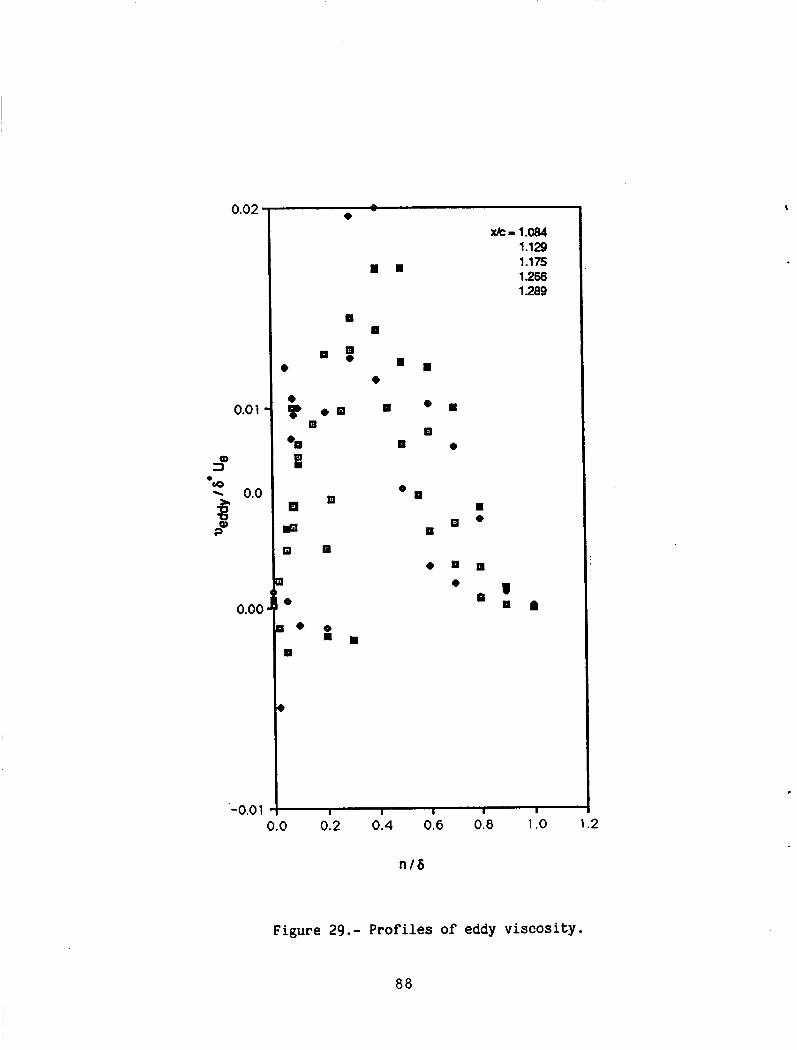
0.02

0.01

9 + 0.0 s 2"

0.00

Figure 29.- Prof i l e s of eddy v i s c o s i t y .

- 0

xk= 1.084 1.129 1.175 1.266 1289

m =

II ID

l a 8

0 El ID 0 .

Om 0 0

0 = . 0

e e

e m

O m w EI

E l .

0 0 1 3

IP II

r a n

U a 0

0 p , n

88

-0.0 1

0 0 0 9 .

II

0

I I I I I

Report Documentation Page I

1. Report No. 2. Government Accession No.

NASA TM-100046

4. Title and Subtitle

.

17. Key Words (Suggested by Authorls))

Separating confluent boundary layer Multi-element airfoil 3-D laser velocimeter

18. Distribution Statement

Unclassified - Unlimited

Subject category - 34

Characteristics of a Separating Confluent Boundary Layer and the Downstream Wake

19. Security Classif. (of this report)

Unclassified

7. Authorfs)

Desmond Adair* and W. Clifton Horne

20. Security Classif. (of this page) 21. No. of pages 22. Price

Unclassified 90 A05

I 9. Performing Organization Name and Address

Ames Research Center Moffett Field, CA 94035

12. Sponsoring Agency Name and Address

National Aeronautics and Space Administration Washington, DC 20546-0001

3. Recipient's Catalog No.

-1 5. Report Date

December 1987 __

6. Performing Organization Code

8. Performing Organization Report No.

A-88034

10. Work Unit No.

505-60-1 1

11. Contract or Grant No.

13. Type of Report and Period Covered

Technical Memorandum 14. Sponsoring Agency Code

15. Supplementary Notes

*NRC Associate Point of Contact: Desmond Adair, Ames Research Center, MS 247-2, Moffett Field, CA 94035

(415) 694-5038 or FTS 464-5038