Characterisation of the Morphological and Surface...

Characterisation of the Morphological and Surface

Properties of Organic Micro-Crystalline Particles

by

Siti Nurul’Ain Yusop

Submitted in accordance with the requirements for the degree of

DOCTOR OF PHILOSOPHY

(CHEMICAL ENGINEERING)

UNIVERSITY OF LEEDS

Institute of Particle Science & Engineering

School of Chemical and Process Engineering

December 2014

i

This copy has been supplied on the understanding that it is copyright

material and that no quotation from the thesis may be published without

proper acknowledgement

Declaration

The work reported in this thesis was carried out in the Institute of Particle

Science and Engineering at the University of Leeds and Diamond Light

Source, Oxfordshire between January 2011 and December 2014 under

supervision of Prof. Kevin J. Roberts and Dr. Vasuki Ramachandran,

together with Dr. Gwyndaf Evans from the Diamond Light Source. The

candidate confirms that the work submitted is her own and that appropriate

credit has been given where reference has been made to the work of

others.

© 2015 The University of Leeds and Siti Nurul’Ain Yusop

ii

Acknowledgements

I would like to thank my supervisors, Prof. Kevin J. Roberts, Dr. Vasuki

Ramachandran and Dr. Gwyndaf Evans from Diamond Light Source for

giving me the opportunity to carry out this PhD project at the University of

Leeds. I much appreciate their constant support, outstanding help and

valuable advice which has enabled me to complete this work.

I would like to acknowledge my research group members in Institute of

Particle Science and Engineering, Dr. David R. Merrifield for his willingness

to assist me on using Inverse Gas Chromatography instrument and his

valuable advice on my work, Miss Thai Thu Hien Nguyen, Miss Siti Fatimah

Ibrahim, Dr. Nornizar Anuar and Mr. Mohd Fitri Othman for their continual

supports. I would also like to thank Microfocus beamline I24 team at

Diamond Light Source, notably Dr. Anna Warren and Dr. Richard Gildea for

their outstanding assistance in helping me to carry out the X-ray

microdiffraction and microtomography experiments and analysis at

Diamond. I would like to thank Dr. Roberts Docherty (Pfizer, Sandwich, UK)

for helpful comments and advice concerning the urea simulations.

I would like to express my special appreciation to my thoughtful husband,

Mr. Seth Iskandar bin Haji Abdul Majid, my beloved mother, Ms Halimah

binti Hashim, and all my family members for their endless supports and

prayers throughout this PhD journey. I would also like to acknowledge my

late father, who was encouraged me to pursue this PhD.

Finally, I would like to thank to Diamond Light Source for providing funding

research and synchrotron radiation beamtime associated with this project

and Universiti Teknologi MARA, Malaysia and the Ministry of Higher

Education, Malaysia for their overall sponsorship of this PhD programme.

iii

Abstract

The surface properties of single and agglomerated micro-crystals are

characterised using the micro-focus X-ray beams available at a third

generation synchrotron light source together with other laboratory facilities.

The influence of the crystallisation environment, on the resultant product

crystals is studied by both varying the cooling rates during crystallisation

and through the addition of impurities and cross-correlated with the

morphology and size changes. Unmodified urea crystallised in 99% ethanol

produce needle-like crystals whilst addition of 4% of biuret in crystallisation

of urea produce a more prismatic crystal shape. At faster cooling rates

smaller sized crystals are produced and vice versa. Dispersive surface

energy analysis using inverse gas chromatography (IGC) shows that

unmodified urea has lower dispersive surface energy than urea modified by

biuret. The dispersive surface energy also increases as the cooling rates

increased. Both the morphology changes and surface energy

measurements are validated using molecular modelling. The morphological

prediction intermolecular force calculations of unmodified urea and urea

modified by biuret are used to calculate a weighted value for the whole

crystals’ dispersive surface energies. The results are in good agreement

with experimental results from IGC. The sorption of urea crystals on water

moisture showed that unmodified urea samples adsorbed water higher than

urea modified by biuret by the observation of the percentage of mass

change with respect to the relative humidity. The study of variability within

powdered samples was found that no significant different in the unit cell

parameters values of each single crystals. The orientation relationship

between agglomerated micro-crystalline particles of aspirin showed the

agglomerates tend to interact at the faces that have ability to form bonding.

In urea samples, most of the agglomerates are mostly aligned due to

epitaxy growth of the crystals. The XMT experiment also was carried out on

agglomerated α-LGA and the 3-dimensional (3D) shape the samples were

obtained.

iv

Table of Contents

Acknowledgements…………………………………………………………ii

Abstract………………………………………………………………………iii

Table of Contents…………………………………………………………..iv

List of Tables ………………………………………………………………viii

List of Figures……………………………………………………………….xi

Notation……………………………………………………………………xvii

Chapter 1 Introduction……………………………………………………1

1.1 Research Background…………………………………………...2

1.2 Research Objectives……………………………………………..4

1.3 Project Management……………………………………………..7

1.4 Structure of the Report…………………………………………..7

References…………………………………………………………….9

Chapter 2 Crystallography Crystallisation & Crystal

Properties……………………………………………………………10

2.1 Introduction………………………………………………………11

2.2 Basic Crystallography…………………………………………..11

2.2.1 Crystal Lattice……………………………………………11

2.2.2 Crystallographic Directions & Planes………………….14

2.2.3 Crystal Projection………………………………………..15

2.2.3.1 Constructions using a Wulff Net……………...17

2.2.4 Atomic Packing…………………………………………..19

2.2.5 Crystal Defects…………………………………………..23

2.3 Crystal Morphology & Habit……………………………………25

2.4 Polymorphism…………………………………………………...26

2.5 Crystallisation……………………………………………………30

2.5.1 Supersaturation………………………………………….30

2.5.2 Metastable Zone Width (MSZW) ………………………31

2.5.3 Nucleation………………………………………………..33

2.5.4 Crystal Growth…………………………………………...33

2.5.5 Types of Crystal Faces………………………………….35

2.6 Agglomeration…………………………………………………...36

2.7 Closing Remarks………………………………………………..37

v

References…………………………………………………………...38

Chapter 3 Surface and Solid State Analysis and

Characterisation of Micro-crystals……………………………..41

3.1 Introduction………………………………………………………42

3.2 Surface Analysis Techniques………………………………….42

3.2.1 Inverse Gas Chromatography (iGC) for

Surface Energy Analysis……………………………......42

3.2.2 Dynamic Vapour Sorption……………………………….49

3.3 X-ray Techniques……………………………………………….50

3.3.1 X-ray Diffraction…………………………………………..50

3.3.1.1 Single Crystal X-ray Diffraction………………...54

3.3.1.2 Reciprocal Lattice………………………………..55

3.3.2 X-ray Tomography ………………………………………56

3.3.3 Synchrotron Radiation…………………………………..57

3.3.3.1 Development of Synchrotron Radiation………58

First Generation of Storage Rings……………..58

Second Generation of Storage Rings…………58

Third Generation of Storage Rings………….…58

3.3.3.2 Overview of Synchrotron Radiation Source…..60

3.4 Closing Remarks………………………………………………..62

References…………………………………………………………...62

Chapter 4 Materials & Methods………………………………………..68

4.1 Introduction………………………………………………………69

4.2 Materials…………………………………………………………69

4.2.1 Urea……………………………………………………….69

4.2.2 Biuret………………………………………………………71

4.2.3 Aspirin……………………………………………………..71

4.2.4 L-Glutamic Acid…………………………………………..73

4.3 Experimental Methods………………………………………….74

4.3.1 Crystallisation of Urea and Urea Modified

by Biuret using AutoMATE………………………………74

4.3.2 Particle Size & Shape Analysis using

Morphologi G3……………………………………………76

vi

4.3.3 Surface Energy Analysis by using

Inverse Gas Chromatography…………………………..77

4.3.4 Water Sorption Isotherm Measurement……………….78

4.3.5 Development of X-ray Microdiffraction (XMD)

and X-ray Microtomography (XMT) Analysis

from Synchrotron…………………………………………79

4.3.5.1 Micromanipulator for Mounting Crystals……...80

4.3.5.2 Sample Preparation……………………………..81

4.3.5.3 Diffraction data Collection and Processing…...82

4.3.5.4 Calculation to Determine Unit Cell

Constants of the Crystals…………………….83

4.3.6 X-Ray Microtomography Instrument…………………...84

4.4 Computational Modeling Methods……………………………85

4.4.1 Calculation of Intermolecular Interaction Using

HABIT98 and Visual Habit………………………………85

4.4.2 Charges Calculation……………………………………..87

4.4.3 Surface Energy Prediction……………………………...87

4.5 Closing Remarks……………………………………………….88

References…………………………………………………………..89

Chapter 5 Influence of Crystallisation Environment on Surface Properties of Urea…………………………………………………92

5.1 Introduction……………………………………………………...93

5.2 Experimental Studies…………………………………………..93

5.2.1 Morphological Habit Measurement Using

Morphologi G3…………………………………...……….93

5.2.2 Surface Energy Analysis Study Using Inverse Gas Chromatography………………………………………....99

5.2.3 Dynamic Vapour Sorption Studies……………………102

5.2.4 Integration of the Experimental Analysis…………….106

5.3 Surface Characterisation using Molecular Modeling……...107

5.3.1 Morphology Prediction of Urea………………………..108

5.3.1.1 Identification of Key Intermolecular

Interactions……………………………………….108

vii

5.3.1.2 Attachment Energy Calculation for

Morphology Prediction………………………..110

5.3.2 Re-evaluation of Intermolecular Potential

Selection for Dispersive Surface Energy Prediction..113

5.3.3 Prediction of Dispersive Surface Energy…………….119

5.3.3.1 Calculations of Fractional Surface

Areas based on Experimental Data……………119

5.4 Discussion…………………………………………………......123

5.5 Closing Remarks………………………………………………124

5.9 References…………………………………………………….124

Chapter 6 Characterisation of Micro-crystals and the

Agglomerates using X-ray Microdiffraction

and Microtomography………………………………………..125

6.1 Introduction…………………………………………………….126

6.2 Justification on Selection of the Materials………………….126

6.3 Case Study 1: Variability in the Structure of

Micro-crystals within Powdered Samples…………………..126

6.3.1 Variation in aspirin powder samples………………….126

6.3.2 Variability in the structure of micro-crystals

as a function of processing conditions……………….127

6.4 Case Study 2: Determination of the Orientation

Relationship between Micro-crystals within

Agglomerates………………………………………………….138

6.4.1 Development of a Stereographic Projection

Method for Agglomerated Micro-crystals…………..139

6.4.2 Agglomerated Aspirin………………………………….142

6.4.3 Agglomerated unmodified urea and urea

modified by Biuret as prepared at different

cooling rates…………………………………………….148

6.5 Case Study 3: Studies of the Polymorphic forms

and transformation of L-glutamic acid………………………164

6.5.1 Crystallisation of L-glutamic acid polymorphic

forms……………………………………………………..164

6.5.2 The Change of Unit Cell Parameters in Mediated

viii

Polymorphic Transformation Crystal of

L-glutamic acid………………………………………….165

6.5.3 Angle Calculations between the contacting

two polymorphs resulting from the transformation

between α- and β- forms of LGA ……………………..168

6.6 Case Study 4: Characterising the 3D shape of

an Agglomerate of α-LGA using X-ray

Microtmography……………………………………………….171

6.6.1 X-ray Microdiffraction data of agglomerated

α-LGA……………………………………………………176

6.7 Discussion ……………………………………………………..178

6.8 Closing Remarks………………………………………………178

References…………………………………………………………178

Chapter 7 Conclusion & Future Works………………………………...181

7.1 Introduction…………………………………………………….182

7.2 Conclusion of this Study ……………………………………..182

7.2.1 Influence of Crystallisation Environment on the

Physico-chemical Properties of Urea Crystals………182

7.2.2 XMD and XMT Studies of the Structure and

Orientation of Single Agglomerated

Micro-crystals……………………………………………183

7.3 Re-appraisal of Thesis Objective…………………………...184

7.4 Suggestion for Future Work…………………………………185

Appendix………………………………………………………………xxviii

ix

List of Tables

Table 2.1 Seven Crystal Systems 12

Table 2.2 Bravais lattice from seven main crystal systems 13

Table 4.1 The coordinates of the unit cell axis for aspirin crystals 83

Table 5.1 Surface energies calculation for set of urea samples

at 0.1oC/min left overnight to undergo slow

cooling crystallisation 100

Table 5.2 Summary of dispersive surface energy results for

unmodified urea and urea modified by biuret at

different cooling rates 101

Table 5.3 Debug analysis of intermolecular bonds in urea using

Hagler force field with Hagler charges 109

Table 5.4 Summary of slice energy and attachment energy using

bulk-isolated charges 111

Table 5.5 Attachment energies of four important faces of

urea calculated using bulk-isolated charges model

for prediction of polar morphology 112

Table 5.6 Description of types of atoms use in lattice

energy calculations for three Hamiltonian parameters

of MOPAC charges (AM1, MNDO, PM3), ab-anitio

charges from CRYSTAL, and Hagler scaled charges

from its own partial charges 114

Table 5.7 Types of charges use in lattice energy calculations.

Three types of charges; empirical charges of MOPAC

with different Hamiltanion parameters (AM1, MNDO,PM3),

ab-anitio charges from CRYSTAL, and Hagler

scaled charges 114

Table 5.8 Types of force-fields with their type of potential in

calculating lattice energy 115

Table 5.9 Lattice energies values of urea using four different

charges and force-fields. The bold columns in black

is the values using Hagler potential with its scaled

charges providing good match to the experimental

x

lattice energy of -22.2 kcal/mol, however, provides

an unrealistically low van der Waals component.

The bold columns in red is the values using

Dreiding potential with CRYSTAL charges, which gives

the highest value of van der Waals component 116

Table 5.10 Percentage surface area of crystal faces obtained

from Visual Habit 120

Table 5.11 Summary of prediction surface energy of unmodified

urea and urea modified by biuret 121

Table 6.1 Summary of unit cell constant determination for aspirin

crystals 128

Table 6.2 Unit cell constants of urea 0.1oC/min 131

Table 6.3 Unit cell constants of urea-biuret crystals 0.1˚C/min 132


Table 6.5 Unit cell constants of urea-biuret crystals 0.25oC/min 133






Table 6.11 Unit cell constants of urea-biuret crystals1.0oC/min 136

Table 6.12 Summary of unit cell parameters for unmodified urea

and urea modified by biuret crystals at different

cooling rates 136

Table 6.13 Angle calculation of agglomerated aspirin crystals

using vector calculation 143

Table 6.14 Angle determination using stereographic projection

method of agglomerated aspirin (sample 1) 143

Table 6.15 Angle determination using stereographic projection

method of agglomerated aspirin (sample 2) 146

Table 6.16 Angle calculations between agglomerated unmodified

urea 0.1oC/min using vector equation 149


urea 0.1oC/min using stereographic projection 149

xi

Table 6.18 Angle calculations between agglomerated urea modified

by biuret 0.1oC/min using vector equation 151


by biuret 0.1oC/min using stereographic

projection 151


urea 0.5oC/min using vector equation 153


by biuret 0.5oC/min using stereographic projection 153


urea 1.0 oC/min using vector calculation 155


urea 1.0 oC/min using stereographic projection 155


by biuret 1.0oC/min using vector calculation 159


by biuret 1.0oC/min using stereographic projection 159

Table 6.26 Planes use for angle calculations determination 161

Table 6.27 Summary of angle calculations of the agglomerated

unmodified urea and urea modified by biuret crystals.

The samples summarised are chosen based on the

smallest angle value to show the parallelism between

crystals 162

Table 6.28 Unit cell constants results of 2 polymorphic forms of LGA.

The value of unit cell constants of α-LGA indicates the data

collected at α- crystal, near the interface of β-LGA, β-LGA

indicates the data collected at β- crystal, interface indicates

the data collected at the interface of α- and β- crystals, and

inside α inidicates the data collected at α- crystals, far away

from the growing β- crystals 167

Table 6.29 Angles calculations of LGA crystals using vector

calculations 169

Table 6.30 Angles calculations of LGA crystals using stereographic

projections 169

xii

Table 6.31 Unit cell parameters determination of two agglomerated

α-LGA 176

Table 6.32 Angle determination using vector calculations and

stereographic projection method 176

xiii

List of figures

Figure 1.1 Flow diagram of the proposed methodology of the

single analysis 6

Figure 1.2 Schematic diagram of structure of the report 8

Figure 2.1 Diagram of lattice parameters determination of crystal

Lattice 12

Figure 2.2 Designation of a crystal plane by Miller indices 14

FIgure 2.3 Spherical projection of normal to crystal faces 15

Figure 2.4 (a) Construction of pole P normal to the crystal plane.

(b) The angle between two planes is equal to the angle

ø between the two poles 16

Figure 2.5 Construction of stereographic projection by defining

the north and south poles in the circle 17

Figure 2.6 (a) The construction of Wulff net with projection of

latitude and longitude on the sphere of projection,

(b) Wulff net drawn with 2o intervals 18

Figure 2.7 (a) Stereographic projection with projection of two poles

(P1 and P2), (b) measurement of the angle between

two poles using Wulff net. The poles lie on great circle 19

Figure 2.8 Types of atoms arrangement in crystal lattice

(a) ABABAB… arrangement

(b) ABCABCABC… arrangement 20

Figure 2.9 The diagram of type of bonding forces exist in matter 21

Figure 2.10 Lennard-Jones potential diagram 22

Figure 2.11 Four types of point defects in a crystal lattice 24

Figure 2.12 Diagram of dislocations occur in crystal lattice 24

Figure 2.13 A twinning plane 25

Figure 2.14 Types of crystal shapes (a) needle-like shape

(b) prismatic shape of snowflakes 26

Figure 2.15 Two polymorphs of paracetamol (a) form I and

(b) form II show different arrangement of molecules

for crystal packing 27

xiv

Figure 2.16 Solubility curves of two polymorphic forms according

to Ostwald's rule 28

Figure 2.17 Schematic diagrams showing the relationship between

the Gibbs free energy and the temperature T of

two polymorphic inter-relationships A and B

represent metastable and stable polymorphs:

(a) monotropic. TA is melting temperature of metastable A

form and TB is a melting temperature of stable B form

(b) enantiotropic. Metastable A form transforms to B form

when the temperature reaches Tt

(transition temperature) 29

Figure 2.18 Metastable Zone Width diagram shows the

metastable region is in between solubility line

and supersolubility curve. Below solubility line,

no crystallisation occurs, while above supersolubility curve,

the crystal growth occurs instantaneous 32

Figure 2.19 Steps, terrace, kink sites and adsorbed molecule on

crystal surface of crystal growth model 34

Figure 2.20 Step (S), kink (K), flat (F) faces 35

Figure 2.21 Schematic diagram of formation of agglomerates from

a group of particles 36

Figure 3.1 Schematic representation of a RT ln VN versus a.

plot for n-alkanes and polar probes 47

Figure 3.2 Propagation of an electromagnetic wave consisting

of cojoined electric magnetic waves 52

Figure 3.3 Diagram of incident wavelength of Bragg's plane 53

Figure 3.4 Schematic diagram of XRD 53

Figure 3.5 The relationship between the crystal orientation and

the diffraction pattern 55

Figure 3.6 Diagram of (a) diffraction patterns from two-dimensional

arrays (b) relationship between crystal lattice and

reciprocal lattice 56

xv

Figure 3.7 An example of tomography method by slicing the object

into several sections and obtained 3D images from

reconstruction of the slice images 56

Figure 3.8 Schematic diagram of Synchrotron Radiation ring at

Diamond Light Source 60

Figure 4.1 Molecular structure of urea 69

Figure 4.2 Morphology of urea showing the slower growing prismatic

{110} faces and the faster growing {111} and {001} faces 70

Figure 4.3 Molecular structure of biuret 71

Figure 4.4 Molecular structure of aspirin 72

Figure 4.5 The formation of the aspirin-aspirin dimer due to hydrogen

bonds between two carboxylic groups 73

Figure 4.6 Molecular Structure of (a) α- and (b) β-L-glutamic acid 73

Figure 4.7 The crystalliser system of AutoMATE (a) four parallel

reactors (b) close-up image of a reactor showing inlets for

the turbidity probe, a glass stirrer, a temperature detector

and cooling jacket 75

Figure 4.8 The Morphologi G3 Malvern Instrument Unit 76

Figure 4.9 (a) The Inverse Gas Chromatography Instrument from

SMS Co.UK Ltd with solvent oven on the left and

column oven on the right (b) Schematic diagram of the

instrument 77

Figure 4.10 Schematic diagram of dynamic vapour sorption

instrument from SMS Co. UK Ltd 78

Figure 4.11 (a) Experimental hutch of beamline I24 (b) Schematic

diagram of XMD 79

Figure 4.12 The stage developed for micromanipulator for mounting

single crystals. (a) shows three adjustable directions

for micromanipulator (b) adjustable joystick to pick up

the selected crystals 81

Figure 4.13 Sample holder for mounting crystal 82

Figure 4.14 Schematic diagram of XMT on I04 beamline 84

Figure 4.15 Limiting radius determination for lattice energy

calculation 86

xvi

Figure 5.1 Images of unmodified urea and urea modified by biuret

crystals crystallised at 0.1oC/min left overnight taken from

Morphologi G3 94

Figure 5.2 Graphs of (a) frequency curves and (b) undersize curves

of unmodified urea and urea modified by biuret crystallised

at 0.1oC/min for asapect ratio (blue:unmodified urea, green:

urea modified by biuret 95

Figure 5.3 Crystal images of unmodified urea and urea modified at

different cooling rates 96

Figure 5.4 Particle size (aspect ratio) distribution of unmodified urea

and urea modified by biuret at different cooling rates 97

Figure 5.5 Distribution of unmodified urea at different cooling rates

indicates that the length of the crystals decreasing at the

faster cooling rates 99

Figure 5.6 Dispersive surface energy plotted of unmodified urea and

urea modified by biuret at different cooling rates 101

Figure 5.7 Graphs of percent in mass changes of (a) unmodified

urea and (b) urea modified by biuret at different cooling rate

at different relative humidity. Red line represents samples

crystallised at cooling rate 0.1oC/min, green line is for

samples crystallised at cooling rate0.25oC/min, purple line

is for samples crystallised at cooling rate 0.5oC/min, blue line

is for samples crystallised at cooling rate 0.75oC/min, and

orange line is for samples crystallised at 1.0oC/min 103

Figure 5.8 Graphs of percent in mass changes of unmodified urea

and urea modified by biuret at (a) 0.1oC/min and (b)

1.0oC/min. Red line and blue rine represent unmodified

urea sample and urea modified by biuret, respectively 105

Figure 5.9 Atom-atom interaction (a) bond type a (b) bond type b

from DM-analysis (c) the interaction between central

molecule of urea (yellow) with its surrounding molecules 110

Figure 5.10 Graphs of slice energy of {111} and {-1-1-1} 112

xvii

Figure 5.11 Morphology prediction of urea using bulk-isolated charges

to calculate the attachment energies of each faces

including the polar faces of (111) and (-1-1-1) 113

Figure 5.12 Lattice energy plots and its component contributions of

urea crystal using Hagler force field with its parameterised

partial electronic charges 117

Figure 5.13 Lattice energy plots and its component contributions of

urea crystal using Dreiding force field with Crystal

charges 118

Figure 5.14 Comparison of morphology of unmodified urea and urea

modified by biuret from experiment and modeling 119

Figure 5.15 Cleave surfacaes of urea with showing of hydrogen

bonding interactions (a) (001) face, (b) (110) face,

(c) (111) face, (d) face 122

Figure 6.1 Aspirin crystal structure visualised in CAMERON graphical

tool plugged-in WinGX software 130

Figure 6.2 Diagram of Wulff net used for determine the angle

between planes and directions of crystals 140

Figure 6.3 Example of stereographic projection result on

agglomerated urea crystals. Blue and red spots indicate

the projected plane for crystal 1 and 2. Green circles

around the (110) plane of both crystals are selected

planes to be used to calculate the angle between planes 141

Figure 6.4 Example of stereographic projection result on

agglomerated urea crystals. Blue and red spots indicate

the projected plane for crystal 1 and 2. Green circles

around the (110) plane of both crystals are selected planes

to be used to calculate the angle between planes.

The Wulff net is overlayed on the projected plot and rotated

to calculate the angle between the planes by aligning two

planes on the great circle 142

Figure 6.5 Image of 2 agglomerated aspirin crystals taken at

beamline 124 DLS 143

xviii

Figure 6.6 Image of 3 aspirin crystals agglomerated captured from

beamline 124 DLS 143

Figure 6.7 Stereographic projection plots of agglomerated aspirin

crystals sample no.1 (sample j and k) 144

Figure 6.8 Stereographic projection plots for aspirin crystals

samples no.2 (sample m & n) 145

Figure 6.9 Sterographic projection plots for aspirin crystals

samples no.2: (sample n and o) 145

Figure 6.10 Morphology prediction of aspirin based on attachment

energy 147

Figure 6.11 The cleave surfaces of aspirin at (100), (b) (110),

and (c) (001) 148

Figure 6.12 (a) Image of unmodified urea crystals recrystallised at

0.1oC/min (sample no.5 in Table 6.16 and 6.17).

Blue and red boxes indicate the position of the

agglomerated crystals. The yellow spots indicate the

point where the beam hits the crystal during data collection,

(b) stereographic projections plotted for sample no.5

(blue: crystal 5p & red: crystal 5q) 150

Figure 6.13 (a) Image of urea modified by biuret crystals

recrystallised at 0.1oC/min (sample no.8 in Table 6.18

and 6.19) Blue and red boxes indicate the position of the

agglomerated crystals. Yellow spots indicate the point

where the beam hits the crystal during data collection,


(blue: crystal 8p & red : crystal 8q) 152




agglomerated crystals. The yellow spots indicate the point




xix

Figure 6.15 Stereographic projection plots for sample no.12 in

table 6.22 and 6.33 156







(blue: crystal 13p & red: crystal 13q). Blue dots cannot be

seen in the plotted image because the plots overlapped

with the red dots plotted 157




agglomerated crystals. The yellow spots indicate the

point where the beam hits the crystal during data collection,


(blue: crystal 15p & red: crystal 15q). The blue dots cannot

be seen in the plotted image because the plots overlapped

with red dots plots 158

Figure 6.18 (a) Image of urea modified by biuret crystals

recrystallised at 1.0oC/min (sample no.17 in Table 6.24

and 6.25). Blue and red boxes indicate the position of the





Figure 6.19 The crystals of LGA observed under hot stage

microscope. Prismatic shape belongs to α-LGA and

observable needle-like shape belongs to β-LGA

(in red circles) 164

xx

Figure 6.20 Samples of LGA with β – crystal grows from α-LGA.

The arrow pointed on the point of the beam hits the

interface: (a) sample 1, (b) sample 2, (c)sample 3. 166

Figure 6.21 Stereographic projection plotted for sample no.2 of alpha

(blue) and beta (red) LGA crystals 169

Figure 6.22 Stereographic projection plotted for sample no.3 of alpha

(blue) and beta (red) LGA crystals 170

Figure 6.23 Molecular packing at surface of (a) (021) of beta form,

(b) (101) of α-form, (c) (111) of α-form 171

Figure 6.24 Image of XMT data collection: (a) image of the beam with

the sample in, (b) flat field reference image, (c) image of

the beam with sample after divided each images in

(a) with image in (b). The sample is circled in red 172

Figure 6.25 The images cut into slices in z-direction during

reconstruction 173

Figure 6.26 3D rendering image after reconstruction 174

Figure 6.27 Microscopic image of α-LGA crystals (captured by

microscope camera from Morphologi G3) 175

Figure 6.28 Stereogrpahic projection plots of two agglomerated

α-LGA. Blue dots represent crystal a and red dots

represent crystal b 177

xxi

Notation

Latin Letters

A surface area of the face

AN Acceptor number

c solution concentration

c* equilibrium concentration

Ce equilibrium solubility

Δc driving force

dhkl interplanar spacing

DN Donor number

E Energy , eV

Eatt attachment energy

Elatt lattice energy

Esl slice energy

Fc carrier gas flow rate, ml/min

∆Gads adsorption free energy

∆GDP dispersive interactions

∆GSP special (polar) interactions

h Planck's constant, 4.135 x 10-15 eV.s

i number of crystals

J correction factor for the compressibility of the carrier gas

j number of faces

KA acidity value of solid particle

KD basicity value of solid particle

M Multiplicity

m mass of stationary phase, g

NA Avogadro's constant, 6.023x1023 mol-1

Po outlet pressure

xxii

Pi inlet pressure

R universal gas constant, 8.314 J/mol.K

r radius of nucleus

rc critical radius of nucleus

S Supersaturation

SA fractional surface area of the (hkl) face

T temperature of the column, K

Tm melting point

T1 undercooled temperature

tG time of first appearance of crystal growth

tN time of first formation of critical nucleus

tr residence time

to hold-up time of non-retained compound (methane), min

t1 time of first appearance of the crystal

VB Buckingham potential

Vcell cell volume of the crystal, m3

VLJ Lennard-jones potential

VN net retention volume

Vs specific retention volume

Wa work of adhesion

Wc work of cohesion

Z number of unit cell

xxiii

Greek Letters

α unit cell angle, o

β unit cell angle, o

ϵ depth of the potential well

σ finite distance at which the inter-particle potential is zero

σ relative supersaturation

θ scattering angle of the diffraction wavelength

υ Frequency

γ unit cell angle, o

γ surface energy, mJ/m2

γd dispersive surface energy for non-polar components

γP surface energy for polar components

γL+ acidic parameter of the probe molecule

γL- basic parameter of the probe molecule

γs+ acidic parameter of the solid surface

γs- basic parameter of the solid surface

dispersive surface energy of solid

dispersive surface energy of probe

λ spreading coefficient

λ Wavelength

xxiv

Abbreviations

BFDH Bravais-Friedel-Donnay-Harker

CCD charge-coupled device

CCDC Cambridge Crystallographic Data Centre

CIF Crystallographic Information File

CSD Cambridge Structure Database

DVS Dynamic Vapour Sorption

hkl miller indices

IGC Inverse Gas Chromatography

LGA L-glutamic acid

MSZW metastable zone width

RF radio frequency

RH relative humidity

SDU sample dispersion unit

XMD X-ray microdiffraction

XMT X-ray microtomography

XDS X-ray Detector Software

XRD X-ray diffraction

1

CHAPTER I

INTRODUCTION

2

1.1 Research Background

Crystallisation is a separation process for preparing fine chemical products.

In the pharmaceutical industry, for example, it is a routine process used to

produce pharmaceutical drug powders. The product performance of the

crystallisation process is dependent on the key processing parameters such

as supersaturation of the solute in the solvent, types of solvent, temperature,

pH, hydrodynamics, cooling rates, etc. These parameters control the

crystallisation process and may affect the polymorphism, size and shape of

the crystals. The surface interfacial properties of the crystals affect the

morphological habit because of the hydrophilic and hydrophobic

characteristics on the individual surface itself. The properties of crystals can

be determined by measuring the powder itself. However, to understand its

surface interfacial properties, it is crucial to measure at the single particle

level. It is because it effects on the physico-chemical properties, that it also

influences the stability and product performance. The characteristics of

individual faces of the crystal determine the surface energy of the crystal.

Each individual facet of the crystal may have different surface energies,

depending upon the relative hydrophilicity and hydrophobicity of the surface.

Traditionally, surface analysis techniques for powder characterisation such

as inverse gas chromatography (IGC) and dynamic vapour sorption (DVS)

analyse surface properties of all the surfaces on the crystals and a net value

which lacks the granularity to be able to assess how process induced

changes to the external shape might impact on the powder’s surface energy.

Theoretically, the surface energy of a sample of facetted crystalline particles

can be defined as (Hammond, et al., 2006):

Surface energy of a particle, γ j (1.1)

Where i is a number of crystals

j represents a unique crystallographic forms on a facetted crystal

number of faces

Mj is a multiplicity of the individual forms

Aj is fractional surface area of the jth face

Sj is a surface energy of the jth face

3

Many pharmaceutical and fine chemical manufacturing processes

produce in micron-sized crystals. In previous studies, the investigation of

surface properties of crystals has been restricted to study on single large

crystals (York, 1983). However, in industry, the particles produced can be

quite small as 20µm and, the particles undergo processes such as milling,

granulation, and compression their surfaces are not always well defined. For

example, these downstream processes may break the crystals, thus the

surface properties may change (Ho et al., 2012). However, there is still a

gap to relate the properties of molecular crystals of single particles,

particularly micro-crystals with the bulk powders which normally produced in

the fine industry. Therefore, it is important to study the characteristics of the

small particulates to understand their surface properties. The surface

properties of single crystals can be characterized by using single crystal X-

ray diffraction (XRD). However, in a normal laboratory XRD, a large beam

size is present which is more suitable for large crystal sizes. Hence, to

understand the structure of agglomerates of micron-sized crystals, a small

beam size is highly preferable as the beam should be smaller than sample to

avoid unwanted air scattering (Evans, 1999). The micro-focus beams

available at third generation of synchrotron radiation facilities provide a

higher intensity and much brighter source of X-rays which is very suitable for

small molecules size crystals (Harding, 1995). In particular, the small beam

sizes (ca 5-10µm) provided enable X-ray microdiffraction (XMD) technique to

be used to study the individual crystals structure within microcrystalline

agglomerates. This technique has been proved in preliminary study of micro-

crystalline organic crystals of aspirin done by Merrifield et al., 2011.

In a similar manner X-ray microtomography (XMT) has been used

previously for the characterisation of small particles. Mostly, though, its use

has been restricted to inorganic systems and at a particle size somewhat

larger than the size of particles envisaged for this study. In previous

research small particle characterisation is well explored (Marks, 1994).

However, there is still a lack of understanding about the structure of

particulate assemblies in particular the relative orientation behaviour

between the constituent crystals. The attractive combination of XMT and

4

XMD has the potential to characterise the external shape of the crystal, its

internal structure and its crystal orientation of within micron-sized

agglomerated crystals (ca. 20-50μm).

1.2 Research Aims and Objectives

In this project, a new holistic approach (see figure 1.1) for the

characterisation micro crystalline samples has been developed

encompassing a combination of XMT and XMD using the Diamond

synchrotron radiation source used in combination with laboratory

characterisation facilities and molecular modelling. Synchrotron radiation is

chosen because it has micron-sized beams that are precisely focused as

well as higher fluxes than laboratory sources enabling the characterisation of

smaller particles. The research question underlying this PhD study is as

follows:

“How the crystal morphology can influence the surface properties of micro-

crystalline particles and how the interactions between particles can be

measured, hence compared between single micro-particle and powdered

samples?”

Delivery of the thesis’s aim will be enabled through a number of key

objectives:

Developing a handling system to help in selection of the samples and

to mount samples on the goniometer for the analysis. Using this, it is

possible to measure the crystal shape, structure, and orientation,

thus, avoiding the problem of selecting new samples, or time

consuming transfer of the sample from one instrument to another.

Examining the morphological habit, particle size and shape

distribution, water sorption effect on the crystals and the surface

energetic nature of crystals using Morphologi G3, Dynamic Vapour

Sorption (DVS) and Inverse Gas Chromatography (iGC).

5

Analysis of surface interfacial properties of micro-crystalline particles,

being the shape, structure and relative orientations of the particles

when they are in agglomerated state using new developing technique

of XMT and XMD in synchrotron radiation source beamline I24,

Diamond Light Source UK.

Assessment of the relationship between bulk properties of the crystals

and the single molecular crystals using molecular modelling of the

intermolecular interactions within the crystal.

6

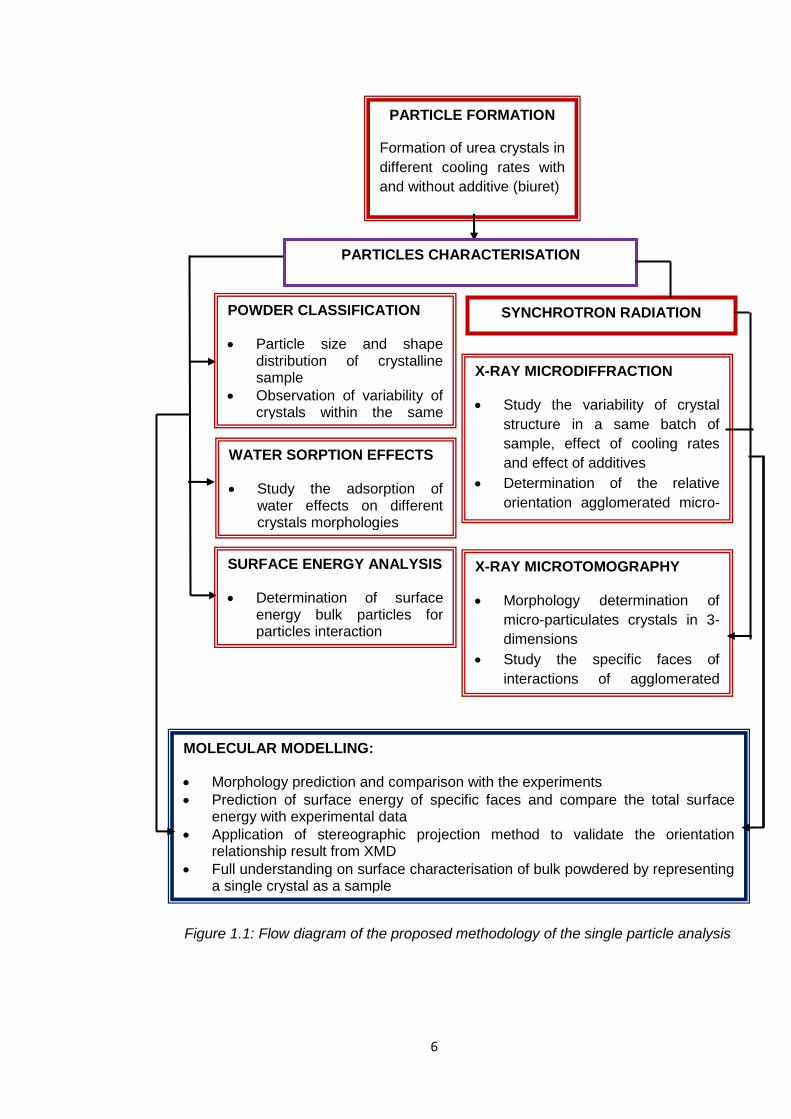
Figure 1.1: Flow diagram of the proposed methodology of the single particle analysis

PARTICLE FORMATION

Formation of urea crystals in

different cooling rates with

and without additive (biuret)

POWDER CLASSIFICATION

Particle size and shape distribution of crystalline sample

Observation of variability of crystals within the same batch of a sample

PARTICLES CHARACTERISATION

SURFACE ENERGY ANALYSIS

Determination of surface energy bulk particles for particles interaction

SYNCHROTRON RADIATION

X-RAY MICRODIFFRACTION

Study the variability of crystal

structure in a same batch of

sample, effect of cooling rates

and effect of additives

Determination of the relative

orientation agglomerated micro-

particulates

X-RAY MICROTOMOGRAPHY

Morphology determination of

micro-particulates crystals in 3-

dimensions

Study the specific faces of

interactions of agglomerated

micro-particulates

MOLECULAR MODELLING:

Morphology prediction and comparison with the experiments

Prediction of surface energy of specific faces and compare the total surface energy with experimental data

Application of stereographic projection method to validate the orientation relationship result from XMD

Full understanding on surface characterisation of bulk powdered by representing a single crystal as a sample

WATER SORPTION EFFECTS

Study the adsorption of water effects on different crystals morphologies

Figure 1.1: Flow diagram of the proposed methodology of the single particle analysis

7

1.3 Project Management

This research project was supervised by Prof. Kevin J. Roberts and Dr.

Vasuki Ramachandran at the University of Leeds, UK in collaboration with

Dr. Gwyndaf Evans at the Synchrotron Radiation Institute, Diamond Light

Source (DLS), Didcot, Oxfordshire, UK. The latter provided a research grant

and synchrotron radiation time at the beamline I24 and I04. The main idea

of this project is to develop a high novelty combination technique of XMD

and XMT at microfocus beamline I24. This project is supervised by:

1. Prof. Kevin J. Roberts, University of Leeds, UK

2. Dr. Gwyndaf Evans, DLS

3. Dr. Vasuki Ramachandran, University of Leeds, UK

The research also involved the team from beamline I24, at the Diamond

Light Source, Dr. Anna Warren for XMD and XMT data collection and Dr.

Richard Gildea who developed the stereographic projection program for

agglomeration data analysis. The laboratory work for surface analysis was

involved Dr. David R. Merrifield who supported in work using inverse gas

chromatography and dynamic vapour sorption. The funding for the study in

four years period funded by Ministry of Higher Education of Malaysia and

Universiti Teknologi MARA (UiTM), Malaysia.

1.4 Structure of the Report

The report is divided into seven chapters (figure 1.2). Chapter I describes

the research background and the aims and objectives of the research.

Chapter II and III explain the fundamental of crystallography and

crystallisation and also the principles of the techniques used in this study.

Chapter IV provides information about the materials and methods used in

this study. Chapter V discusses the experimental results and molecular

modelling simulation on the effect of morphology of urea influenced by

different process conditions. Chapter VI discusses the XMD and XMT

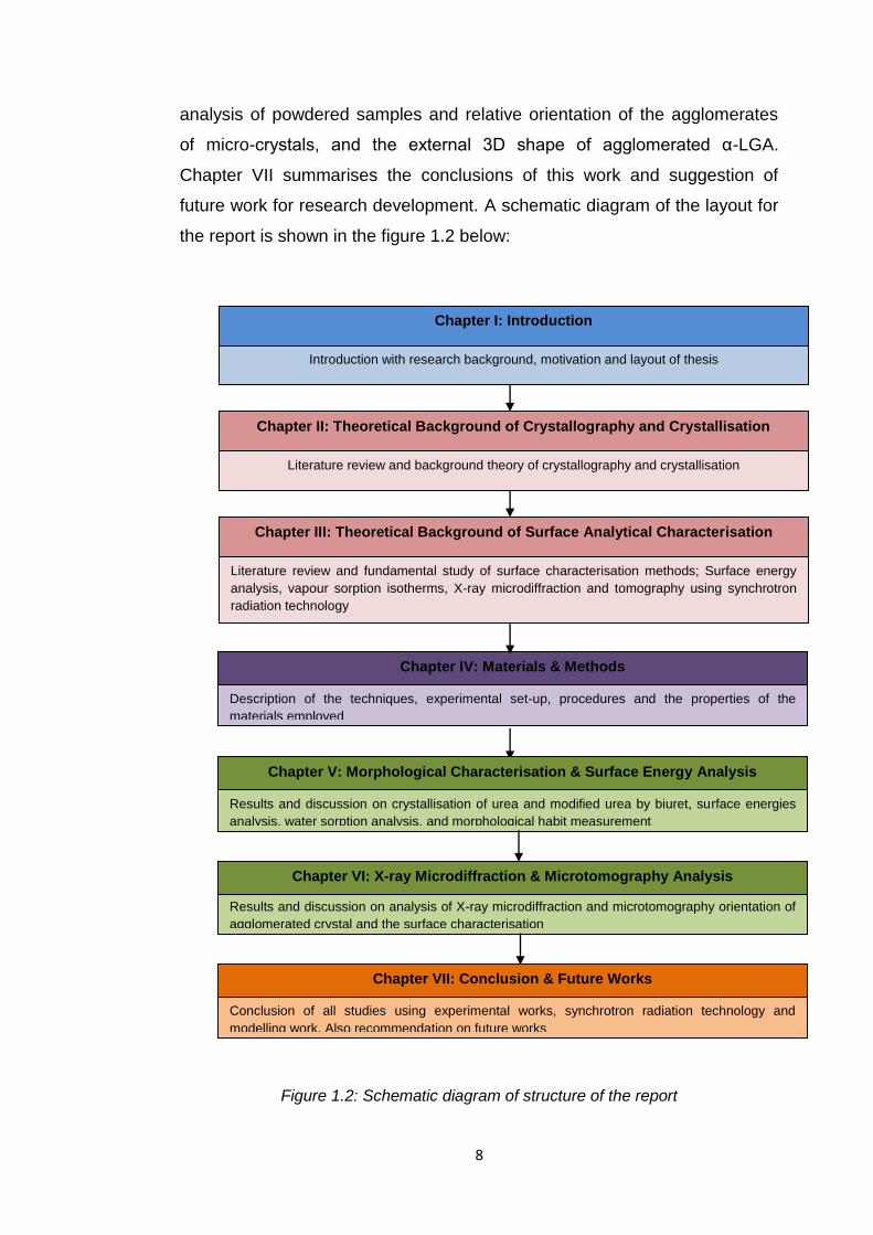
8

analysis of powdered samples and relative orientation of the agglomerates

of micro-crystals, and the external 3D shape of agglomerated α-LGA.

Chapter VII summarises the conclusions of this work and suggestion of

future work for research development. A schematic diagram of the layout for

the report is shown in the figure 1.2 below:

Figure 1.2: Schematic diagram of structure of the report

Literature review and background theory of crystallography and crystallisation

Literature review and fundamental study of surface characterisation methods; Surface energy

analysis, vapour sorption isotherms, X-ray microdiffraction and tomography using synchrotron

radiation technology

Chapter I: Introduction

Chapter II: Theoretical Background of Crystallography and Crystallisation

Chapter III: Theoretical Background of Surface Analytical Characterisation

Introduction with research background, motivation and layout of thesis

Description of the techniques, experimental set-up, procedures and the properties of the

materials employed

Chapter IV: Materials & Methods

Results and discussion on crystallisation of urea and modified urea by biuret, surface energies

analysis, water sorption analysis, and morphological habit measurement

Chapter V: Morphological Characterisation & Surface Energy Analysis

Results and discussion on analysis of X-ray microdiffraction and microtomography orientation of

agglomerated crystal and the surface characterisation

Chapter VI: X-ray Microdiffraction & Microtomography Analysis

Conclusion of all studies using experimental works, synchrotron radiation technology and

modelling work. Also recommendation on future works

Chapter VII: Conclusion & Future Works

9

References

1. Evans, P.R., (1999). Some Notes on Choices in Data Collection. Act.

Cryst. (D) (55):1771-1772.

2. Harding, M.M., (1995). Synchrotron Radiation-New Opportunities for

Chemical Crystallography. Act Crystallogr. B. (51):432-446.

3. Ho, R., Naderi, M., Heng, J.Y.Y., Williams, D.R., Thielmann, F.,

Bouza, P., Keith, A.R., Thiele, G., Burnett, D.,J., (2012). Effect of

Milling on Particle Shape and Surface Heterogeneity of Needle-

Shaped Crystals. Pharm. Res. (29) 2806-2816.

4. Merrifield, D.R., Ramachandran, V., Roberts, K.J., Armour, W.,

Axford, D., Basham, M., Connolley, T., Evans, G., McAuley, K.E.,

Owen, R.L., Sandy, J., (2011). A Novel Technique Combining High-

Resolution Synchrotron X-ray Microtomography and X-ray Diffraction

for Characterisation of Micro-particulates. Meas. Sci.Technol. (22).

5. York, P., (1983). Solid-state Properties of Powders in the formulation

and processing of solid dosage forms. Int. J. Pharm. (14) 1-28.

10

CHAPTER II

CRYSTALLOGRAPHY, CRYSTALLISATION & CRYSTAL

PROPERTIES

11

2.1 Introduction

This chapter discusses the background to the basics of crystallography, the

structure of crystals, how molecules arrange themselves in a crystal lattice

and the bonding forces involved. It also discusses the crystallisation process

which is important in producing particles with desired crystal morphology and

polymorphic form.

2.2 Basic Crystallography

The understanding of the atom distribution in the crystalline state was

discovered by Max Von Laue, W.H. and W.L. Braggs in 1912 (Braggs,

1913). The first X-ray diffraction experiments were carried out by them to

work out the structure of rock salt, whilst W. H. Bragg discovered the

wavelength of monochromatic X-ray beams (Barret & Massalski, 1980). An

ordered arrangement of atoms or molecules which repeats in three-

dimensions forms a crystal. Crystalline materials contain a regular repeating

pattern of atoms or molecules, the smallest repeat of which is known as a

unit cell. A crystal is the most stable form since the energy of the atomic

interaction is at its lowest state compared amorphous material which has a

random arrangement of atoms or molecules. Each crystal has its own shape,

in facets which grow naturally during crystallisation, the shape and faces of

the crystal are dependent on the atoms and molecules inside the crystal.

2.2.1 Crystal Lattice

Crystalline solids form by the long range ordering of atoms in a repeating

pattern called a unit cell. The atoms arrangement is repeated in a specific

direction and distance (Glusker & Trueblood, 2010). The unit cell contains

the information about the atoms coordinates, types of atoms and site

occupancy. The repetition of the unit cell can be represented by the

geometry of the repetition. The lengths (a, b, c) of the unit cell are measured

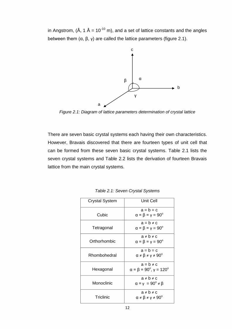
12

in Angstrom, (Å, 1 Å = 10-10 m), and a set of lattice constants and the angles

between them (α, β, γ) are called the lattice parameters (figure 2.1).

Figure 2.1: Diagram of lattice parameters determination of crystal lattice

There are seven basic crystal systems each having their own characteristics.

However, Bravais discovered that there are fourteen types of unit cell that

can be formed from these seven basic crystal systems. Table 2.1 lists the

seven crystal systems and Table 2.2 lists the derivation of fourteen Bravais

lattice from the main crystal systems.

Table 2.1: Seven Crystal Systems

Crystal System Unit Cell

Cubic

a = b = c α = β = γ = 90o

Tetragonal

a = b ≠ c

α = β = γ = 90o

Orthorhombic

a ≠ b ≠ c

α = β = γ = 90o

Rhombohedral

a = b = c α ≠ β ≠ γ ≠ 90o

Hexagonal

a = b ≠ c

α = β = 90o, γ = 120o

Monoclinic

a ≠ b ≠ c

α = γ = 90o ≠ β

Triclinic

a ≠ b ≠ c

α ≠ β ≠ γ ≠ 90o

c

β α

γ

b

a

13

Table 2.2: 14 Bravais lattice from seven main crystal systems

Cubic

Tetragonal Hexagonal

Orthorhombic

Monoclinic

Rhombohedral Triclinic

Primitive (P) Body-centred (I) Face-centred (F)

a

a

a a

a

a a

a

a

a

a

c

Primitive (P) Body-centred (I)

a

a

c a

a

c

a

b

c

Primitive (P) Body-centred (I) Base-centred (C) Face-centred (F)

a

b

c a

b

c a

b

c

Primitive (P)

a

b

c a

b

c

Primitive (P) Base-centred (C)

a

a

a

a

b

c

14

2.2.2 Crystallographic Directions and Planes

All crystal structures have different faces as described as a plane with

specific directions. In crystallography Miller indices form a notation for planes

within a crystal lattice. Figure 2.2 shows a determination of crystal plane in

crystal lattice system (Millburn, 1973).

Figure 2.2: Designation of a crystal plane by Miller indices

The A’ B’ C’ plane is denoted by:

A’ = OA’ B’ = OB’ C’ = OC’

OA OB OC

The plane of Miller indices for the unit cell can be expressed as

,

,

a

b

c

O

A’

B’

C’

A

B

C

D E

F

G

15

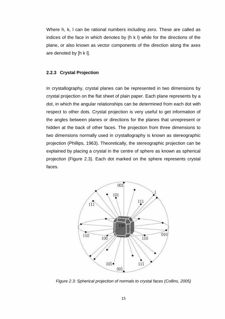
Where h, k, l can be rational numbers including zero. These are called as

indices of the face in which denotes by (h k l) while for the directions of the

plane, or also known as vector components of the direction along the axes

are denoted by [h k l].

2.2.3 Crystal Projection

In crystallography, crystal planes can be represented in two dimensions by

crystal projection on the flat sheet of plain paper. Each plane represents by a

dot, in which the angular relationships can be determined from each dot with

respect to other dots. Crystal projection is very useful to get information of

the angles between planes or directions for the planes that unrepresent or

hidden at the back of other faces. The projection from three dimensions to

two dimensions normally used in crystallography is known as stereographic

projection (Phillips, 1963). Theoretically, the stereographic projection can be

explained by placing a crystal in the centre of sphere as known as spherical

projection (Figure 2.3). Each dot marked on the sphere represents crystal

faces.

Figure 2.3: Spherical projection of normals to crystal faces (Collins, 2005)

16

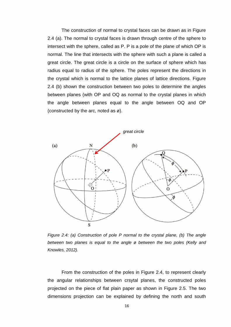
The construction of normal to crystal faces can be drawn as in Figure

2.4 (a). The normal to crystal faces is drawn through centre of the sphere to

intersect with the sphere, called as P. P is a pole of the plane of which OP is

normal. The line that intersects with the sphere with such a plane is called a

great circle. The great circle is a circle on the surface of sphere which has

radius equal to radius of the sphere. The poles represent the directions in

the crystal which is normal to the lattice planes of lattice directions. Figure

2.4 (b) shown the construction between two poles to determine the angles

between planes (with OP and OQ as normal to the crystal planes in which

the angle between planes equal to the angle between OQ and OP

(constructed by the arc, noted as ø).

Figure 2.4: (a) Construction of pole P normal to the crystal plane, (b) The angle

between two planes is equal to the angle ø between the two poles (Kelly and

Knowles, 2012).

From the construction of the poles in Figure 2.4, to represent clearly

the angular relationships between crsytal planes, the constructed poles

projected on the piece of flat plain paper as shown in Figure 2.5. The two

dimensions projection can be explained by defining the north and south

great circle

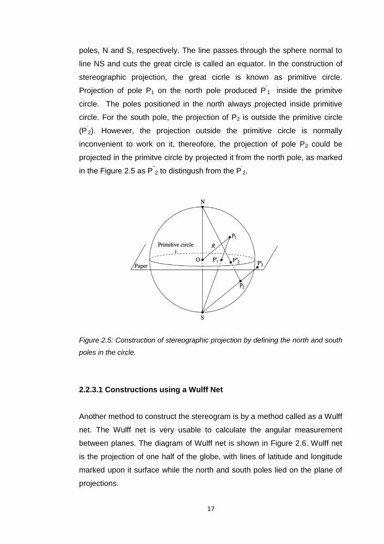
17

poles, N and S, respectively. The line passes through the sphere normal to

line NS and cuts the great circle is called an equator. In the construction of

stereographic projection, the great cicrle is known as primitive circle.

Projection of pole P1 on the north pole produced P’1 inside the primitve

circle. The poles positioned in the north always projected inside primitive

circle. For the south pole, the projection of P2 is outside the primitive circle

(P’2). However, the projection outside the primitive circle is normally

inconvenient to work on it, thereofore, the projection of pole P2 could be

projected in the primitve circle by projected it from the north pole, as marked

in the Figure 2.5 as P’’2 to distingush from the P’

2.

Figure 2.5: Construction of stereographic projection by defining the north and south

poles in the circle.

2.2.3.1 Constructions using a Wulff Net

Another method to construct the stereogram is by a method called as a Wulff

net. The Wulff net is very usable to calculate the angular measurement

between planes. The diagram of Wulff net is shown in Figure 2.6. Wulff net

is the projection of one half of the globe, with lines of latitude and longitude

marked upon it surface while the north and south poles lied on the plane of

projections.

18

(a) (b)

Figure 2.6: (a) The construction of Wulff net with projection of latitude and longitude

on the sphere of projection, (b) Wulff net drawn with 2o intervals (Kelly and

Knowles, 2012).

The net can be used together with the stereogram by placing one on

top of another by using transparent tracing paper in order to measure the

angular relationships between crystal planes, with the equal radius between

both sphere and the location of the centre. The angle between poles within

the primitive circle can be measured by rotating the stereogram until the two

poles lie on the same great circle and the angles measured by counting the

small circles between the poles. The measurement is explained in Figure

2.7.

longitude

latitude

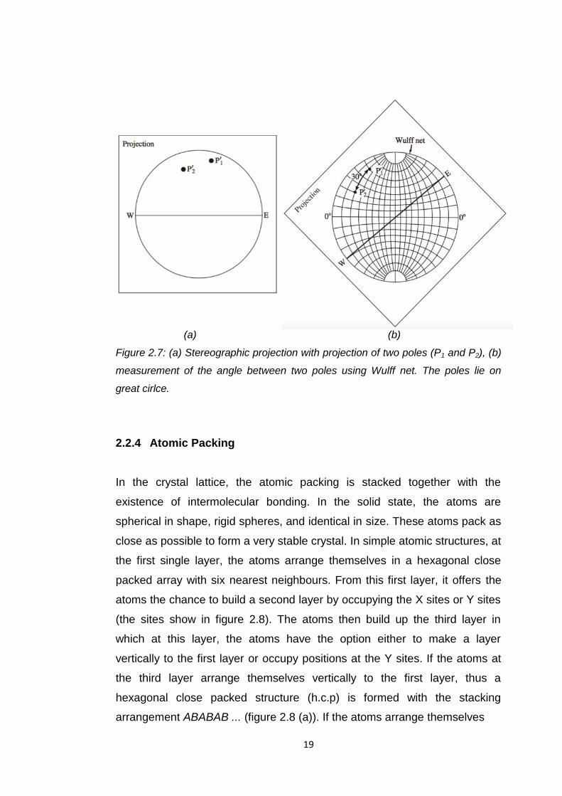
19

(a) (b)

Figure 2.7: (a) Stereographic projection with projection of two poles (P1 and P2), (b)

measurement of the angle between two poles using Wulff net. The poles lie on

great cirlce.

2.2.4 Atomic Packing

In the crystal lattice, the atomic packing is stacked together with the

existence of intermolecular bonding. In the solid state, the atoms are

spherical in shape, rigid spheres, and identical in size. These atoms pack as

close as possible to form a very stable crystal. In simple atomic structures, at

the first single layer, the atoms arrange themselves in a hexagonal close

packed array with six nearest neighbours. From this first layer, it offers the

atoms the chance to build a second layer by occupying the X sites or Y sites

(the sites show in figure 2.8). The atoms then build up the third layer in

which at this layer, the atoms have the option either to make a layer

vertically to the first layer or occupy positions at the Y sites. If the atoms at

the third layer arrange themselves vertically to the first layer, thus a

hexagonal close packed structure (h.c.p) is formed with the stacking

arrangement ABABAB ... (figure 2.8 (a)). If the atoms arrange themselves

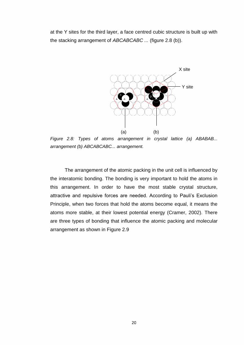
20

at the Y sites for the third layer, a face centred cubic structure is built up with

the stacking arrangement of ABCABCABC ... (figure 2.8 (b)).

Figure 2.8: Types of atoms arrangement in crystal lattice (a) ABABAB...

arrangement (b) ABCABCABC... arrangement.

The arrangement of the atomic packing in the unit cell is influenced by

the interatomic bonding. The bonding is very important to hold the atoms in

this arrangement. In order to have the most stable crystal structure,

attractive and repulsive forces are needed. According to Pauli’s Exclusion

Principle, when two forces that hold the atoms become equal, it means the

atoms more stable, at their lowest potential energy (Cramer, 2002). There

are three types of bonding that influence the atomic packing and molecular

arrangement as shown in Figure 2.9

(a)

X site

Y site

(b)

21

Figure 2.9: The diagram of type of bonding forces exist in matter

Covalent bonding is a chemical bond in which the atoms share the electrons

to complete the outer valency shell. The bond is affected by the

electronegativity of the atoms in which the sharing of electrons between

equal electronegative atoms forms non-polar bonding while unequal

electronegativity causes polar bonding.

Ionic bonding is an attractive force between two different electron

charges; known as cations and anions. The ionic bonding occurs when the

electronegative charged atom releases its electron to achieve a stable

electron configuration while the electropositive charges atom accepts the

released electronegative charges to achieve its stable electron configuration.

The non-bonded interaction, called van der Waals is the weakest

among the three types of bonding and is an intermolecular interaction. It

exists because of the polarisability of an electron orbital. Van der Waals

bonding balances the electronic charge imbalance of ionic and covalent

bonding. There are three types of van der Waals forces:

(i) Keesom force (dipole- dipole interactions)

(ii) Debye force (dipole-induced dipole interactions)

(iii) London dispersion force (induced dipole-induced dipole interactions)

Ionic:

Strong and un-directed

Covalent:

Strong and directed

Bonding Forces

Van der Waals:

Weak and un-directed

Metal:

Mixed and un-directed

Hydrogen:

Weak and directed

22

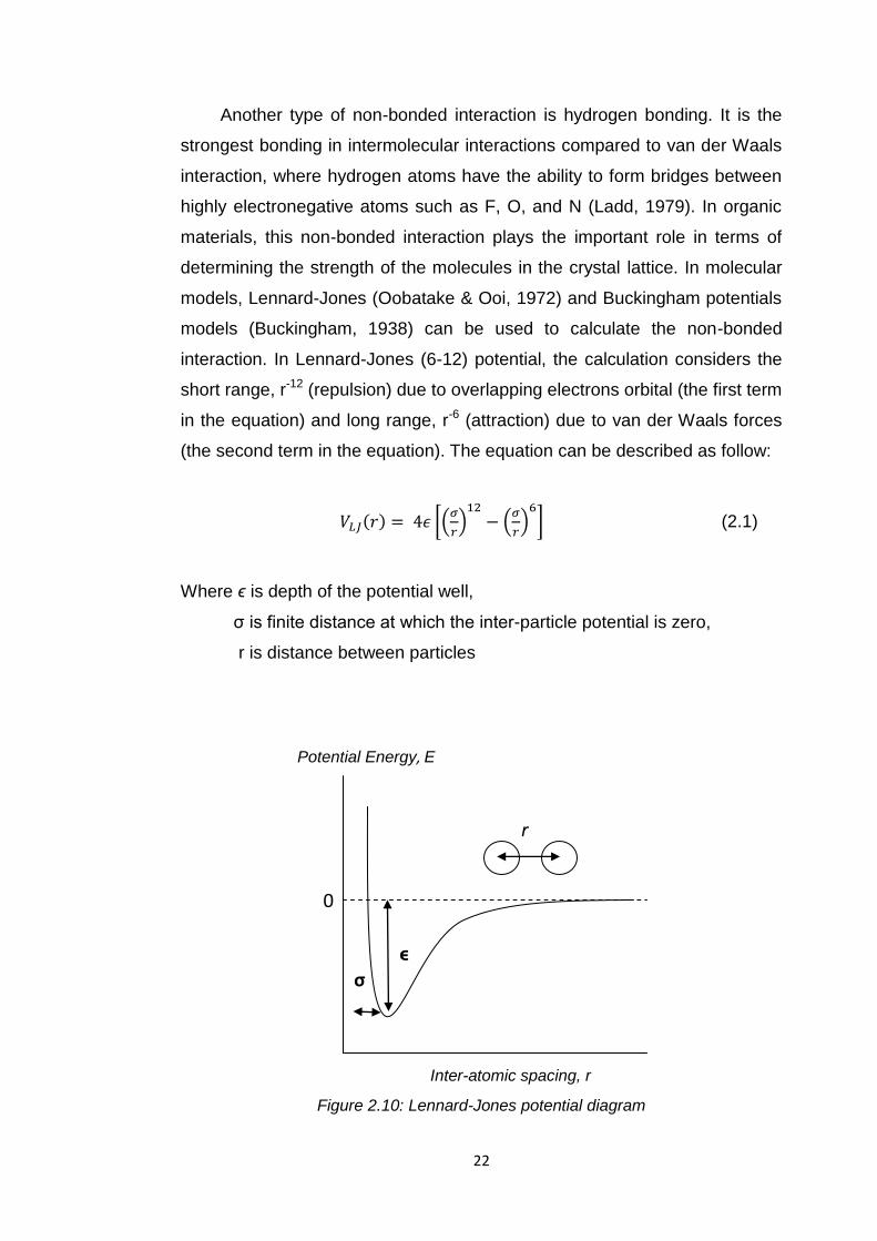
Another type of non-bonded interaction is hydrogen bonding. It is the

strongest bonding in intermolecular interactions compared to van der Waals

interaction, where hydrogen atoms have the ability to form bridges between

highly electronegative atoms such as F, O, and N (Ladd, 1979). In organic

materials, this non-bonded interaction plays the important role in terms of

determining the strength of the molecules in the crystal lattice. In molecular

models, Lennard-Jones (Oobatake & Ooi, 1972) and Buckingham potentials

models (Buckingham, 1938) can be used to calculate the non-bonded

interaction. In Lennard-Jones (6-12) potential, the calculation considers the

short range, r-12 (repulsion) due to overlapping electrons orbital (the first term

in the equation) and long range, r-6 (attraction) due to van der Waals forces

(the second term in the equation). The equation can be described as follow:

(2.1)

Where ϵ is depth of the potential well,

σ is finite distance at which the inter-particle potential is zero,

r is distance between particles

Figure 2.10: Lennard-Jones potential diagram

σ

ϵ

0

Potential Energy, E

Inter-atomic spacing, r

r

23

Figure 2.10 represents Lennard-jones potential which the potential energy

diagrams against the inter-atomic distance, r between the atoms.

Buckingham potential is alternative equation of Lennard-Jones which it

does not take into account the short-range term of the repulsion, thus, the

equation becomes

(2.2)

2.2.5 Crystal Defects

An ideal crystal is one which contains no defects, however, in reality, defects

in crystals always occur. The distortion or irregularity in atomic arrangement

can cause a crystal lattice defect. Defects in crystals are not always

disadvantageous. Defects in crystal lattice can intentionally be introduced to

improve the mechanical properties of a material. There are four types of

crystal defects; (i) point defects (0-D), (ii) linear defects (1-D), (iii) planar

defects (2-D), (iv) bulk defects (3-D).

Point defects (as shown in figure 2.11) occur when an atom is missing

or irregularly placed in the lattice structure. Point defects can occur in four

conditions:

lattice vacancies when the atoms are absent (also called Schottky

defect)

self-interstitials when atoms occupy the positions between ideal lattice

atomic position

substitution impurity atoms in which the atoms replace the host atoms

in specific sites within the crystal lattice

interstitial impurity atoms in which the atoms occupy the interstitial

place in the crystal lattice.

However, it is also possible for the two point defects to occur simultaneously.

For example, the lattice vacancy and self-interstitial atom defects can occur

24

in pairs when the atom moves out to an interstitial position and vacates its

original position. This pair of defects is also called a Frenkel defect.

Figure 2.11: 4 types of point defect in a crystal lattice

Linear defects, commonly known as ‘dislocations’, are defects occur

when some of the atoms are not in their positions in the crystal structure.

There are two primary types of dislocations; (i) edge dislocations (figure 2.12

(i)), (ii) screw dislocations (figure 2.12 (ii)). Sometimes, a combination of

both dislocations may occur, as which is also a common situation in crystal

defects (figure 2.12 (iii)). Burgers vector is used to describe the magnitude of

distortion of the plane. Edge dislocations occur when a line of atoms

terminate its plane in the middle of the crystal lattice. In edge dislocations,

Burgers vector is perpendicular to the line of direction. A screw dislocation

occurs when Burger’s vector is parallel to the dislocation line.

Figure 2.12: Diagram of dislocations occur in crystal lattice

vacancy

substitutional

interstitial

self interstitial

25

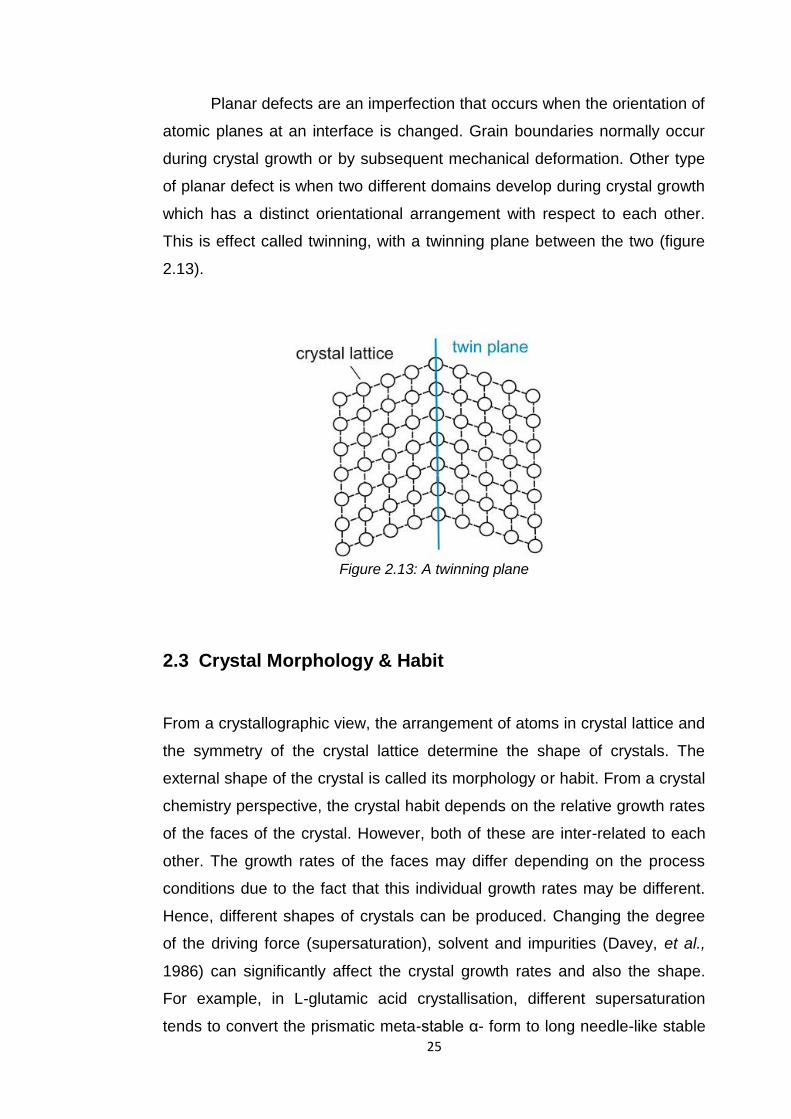
Planar defects are an imperfection that occurs when the orientation of

atomic planes at an interface is changed. Grain boundaries normally occur

during crystal growth or by subsequent mechanical deformation. Other type

of planar defect is when two different domains develop during crystal growth

which has a distinct orientational arrangement with respect to each other.

This is effect called twinning, with a twinning plane between the two (figure

2.13).

Figure 2.13: A twinning plane

2.3 Crystal Morphology & Habit

From a crystallographic view, the arrangement of atoms in crystal lattice and

the symmetry of the crystal lattice determine the shape of crystals. The

external shape of the crystal is called its morphology or habit. From a crystal

chemistry perspective, the crystal habit depends on the relative growth rates

of the faces of the crystal. However, both of these are inter-related to each

other. The growth rates of the faces may differ depending on the process

conditions due to the fact that this individual growth rates may be different.

Hence, different shapes of crystals can be produced. Changing the degree

of the driving force (supersaturation), solvent and impurities (Davey, et al.,

1986) can significantly affect the crystal growth rates and also the shape.

For example, in L-glutamic acid crystallisation, different supersaturation

tends to convert the prismatic meta-stable α- form to long needle-like stable

26

β-form at specific temperature (Ferrari and Davey, 2004). The solvent effect

in crystallization of aspirin shows that if different solvents are used for

crystallisation, hence, may produce different shapes of crystals i.e aspirin

(Watanabe et al., 1982).

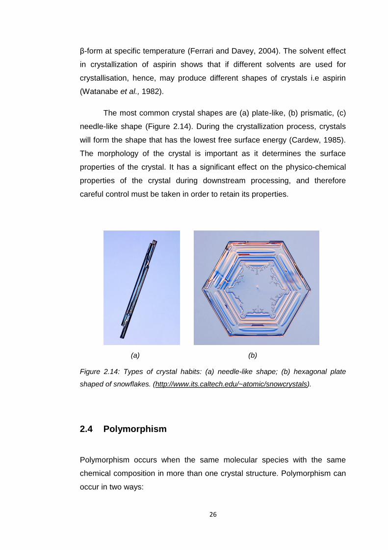
The most common crystal shapes are (a) plate-like, (b) prismatic, (c)

needle-like shape (Figure 2.14). During the crystallization process, crystals

will form the shape that has the lowest free surface energy (Cardew, 1985).

The morphology of the crystal is important as it determines the surface

properties of the crystal. It has a significant effect on the physico-chemical

properties of the crystal during downstream processing, and therefore

careful control must be taken in order to retain its properties.

(a) (b)

Figure 2.14: Types of crystal habits: (a) needle-like shape; (b) hexagonal plate

shaped of snowflakes. (http://www.its.caltech.edu/~atomic/snowcrystals).

2.4 Polymorphism

Polymorphism occurs when the same molecular species with the same

chemical composition in more than one crystal structure. Polymorphism can

occur in two ways:

http://www.its.caltech.edu/~atomic/snowcrystals

27

(1) Packing polymorphisms in which the molecules have different crystal

packing between two polymorphs (Braun, et al., 2008). Figure 2.15

shows the packing polymorphism of paracetamol form I and II.

(2) Conformational polymorphisms in which the molecules flexibly change

their conformation arrangements of the molecules, for example change

in torsion angles of the bonding between atoms or functional group

(Cabeza & Bernstein, 2014).

(a) (b)

Figure 2.15: Two polymorphs of paracetamol (a) form I and (b) form II show

different arrangement of molecules for crystal packing (Redinha et al., 2013).

The formation of different polymorphs can be effected example by

recrystallisation of the compound in different solvents and or through

variation of crystallisation conditions such as temperature, concentration and

pH. (Byrn et al., 1995). For example, crystallisation of hydrocetridine from

different solvents can form crystals with different polymorphs. Different

conditions such as supersaturation and the temperature of crystallisation

process will also affect the crystal morphology even if the same solvents

used (Chen et al., 2008). Polymorphism can also be controlled by using

“tailor made additives”, being either solvents or additives which have similar

molecular structure as the host molecule (Roberts et al., 1994), (Graham et

al., 2013).

28

The formation of polymorphs is important in pharmaceutical processing

as the difference in physical properties can have an impact on the

performance of the pharmaceutical drugs. This is because different

polymorphs can have different physical properties such as molar density,

hygroscopicity, melting temperature, heat capacity, solubility, dissolution

rate, stability, habit, hardness, and compactibility. Thus, fully controlling the

process is very crucial to ensure that only the desired polymorph will form.

Another different case exists when the crystal has incorporated solvent

molecules in its structure (non-solvated crystal). On first examination such

as a situation would appear as if polymorph had been produced. However, it

would not be polymorph but is often called a pseudo-polymorph because the

chemical compositions of the non-solvated and solvated crystals differ

(Giron, 2001).

The existence of polymorphic forms can be affected by either

thermodynamics or kinetics. If the thermodynamic factor determines the

polymorphic formation, the polymorph produced depends on the stability of

the crystal. The most stable form of a polymorph is that which has the lowest

free energies. This can often be characterised by the lowest solubility,

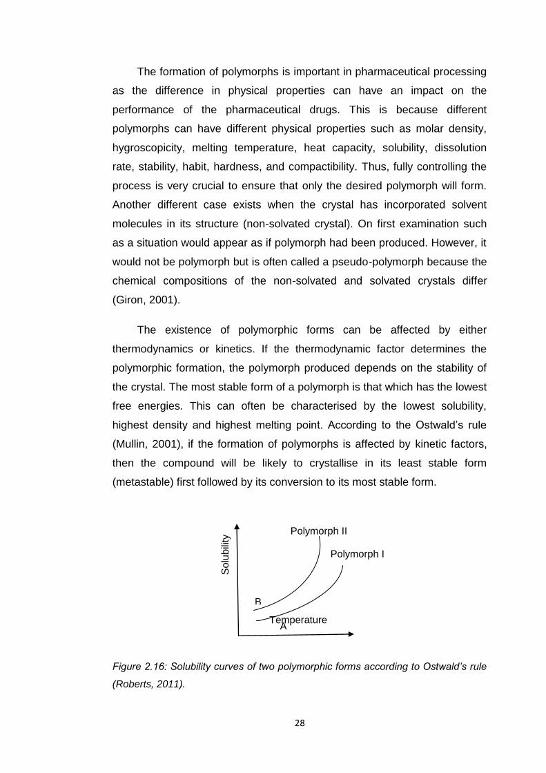
highest density and highest melting point. According to the Ostwald’s rule

(Mullin, 2001), if the formation of polymorphs is affected by kinetic factors,

then the compound will be likely to crystallise in its least stable form

(metastable) first followed by its conversion to its most stable form.

Figure 2.16: Solubility curves of two polymorphic forms according to Ostwald’s rule

(Roberts, 2011).

Temperature

So

lubili

ty

B

o

A

o

Polymorph I

Polymorph II

29

Figure 2.16 above gives an example of the formation of polymorphs I

and II by Ostwald’s rule. Consider that the compound is crystallised in two

different solvents, A and B. Solvent A is supersaturated to polymorph I but

not II, while solvent B is supersaturated with respect to both polymorphs. In

certain conditions, the least stable polymorph form which is polymorph II will

transform to polymorph I which is the most stable form (Mullin, 2001). The

anti-viral HIV drug, Stavudine, has two polymorphic forms. During the

crystallisation, the effect of supersaturation was studied. In agreement with

Ostwald’s rule, Stavudine form I which is is the least stable polymorph

formed first, followed by its conversion to the more stable form II (Mirmehrabi

& Rohani, 2006).

There are two types of structural inter-relationship between polymorphs:

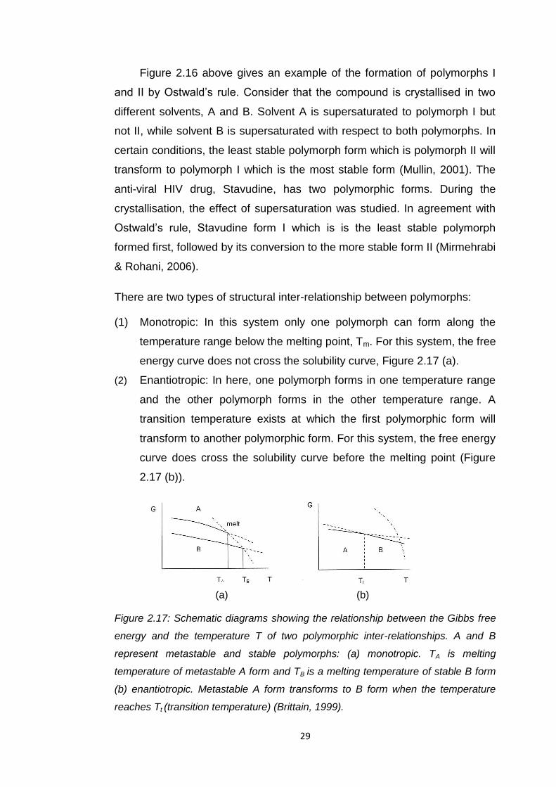
(1) Monotropic: In this system only one polymorph can form along the

temperature range below the melting point, Tm. For this system, the free

energy curve does not cross the solubility curve, Figure 2.17 (a).

(2) Enantiotropic: In here, one polymorph forms in one temperature range

and the other polymorph forms in the other temperature range. A

transition temperature exists at which the first polymorphic form will

transform to another polymorphic form. For this system, the free energy

curve does cross the solubility curve before the melting point (Figure

2.17 (b)).

(a) (b)

Figure 2.17: Schematic diagrams showing the relationship between the Gibbs free

energy and the temperature T of two polymorphic inter-relationships. A and B

represent metastable and stable polymorphs: (a) monotropic. TA is melting

temperature of metastable A form and TB is a melting temperature of stable B form

(b) enantiotropic. Metastable A form transforms to B form when the temperature

reaches Tt (transition temperature) (Brittain, 1999).

30

2.5 Crystallisation

Crystallisation from solution phases is a purification process using

liquid/solid separation techniques which separates a solid from its ‘mother’

solution. In this process, the solution can be formed by the addition of a solid

to the solvent. Depending on the solubility of the solid in the solvent, at

certain temperature and pressure, a homogenous solution can be produced.

When the maximum amount of solute is dissolved in a given volume, the

solution is said to be saturated. Cooling of such a solution can result in

crystallisation process that involves three stages:

(1) Supersaturation

(2) Nucleation

(3) Crystal Growth

2.5.1 Supersaturation

The crystallisation process is dependent on a suitable driving force, i.e

supersaturation. A supersaturated solution in one in which the solute

concentration is higher than solution’s the equilibrium solubility at a given

temperature. ∆c is denoted as the driving force. S, the supersaturation, is the

ratio of actual (c) to equilibrium (c*) solubilities given by:

(2.3)

and

(2.4)

Thus, the absolute or relative supersaturation, σ, can be expressed by:

(2.5)

31

There are a number of ways that can be used to supersaturation to occur:

the temperature of the solution can be changed depending on the

sign of the solubility coefficient.

solution pH can be changed in cases where the solution is an

electrolyte.

evaporation of the solvent. This is a simple technique often used in

the production of non-speciality bulk chemicals.

using a mixture of solvents in which the second added solvent has a

low solubility but highly miscible than the saturating solution prepared

from the first solvent.

2.5.2 Metastable Zone Width (MSZW)

Measurement of the metastable zone width (MSZW) is often used to assess

the nucleation behaviour and solubility of the solute in a specified solvent in

the crystallisation process (Mullin, 2001). The MSZW value can be highly

dependent on process conditions. Factors that influence the value of MSZW

are cooling / supersaturation rate, the purity of the solution and the nature of

the crystals themselves. The presence of nucleation surpressing impurities

can affect the MSZW value which commonly widens the metastable zone.

Changes in temperature can also make the MSZW become broader. For

example, the nucleation behaviour may vary if the temperature of the

solution is maintained at a higher temperature than the equilibrium

temperature for a long period of time, in comparison to the case where the

solution temperature is maintained just above the saturation temperature.

Solution agitation can also be used to narrow the MSZW.

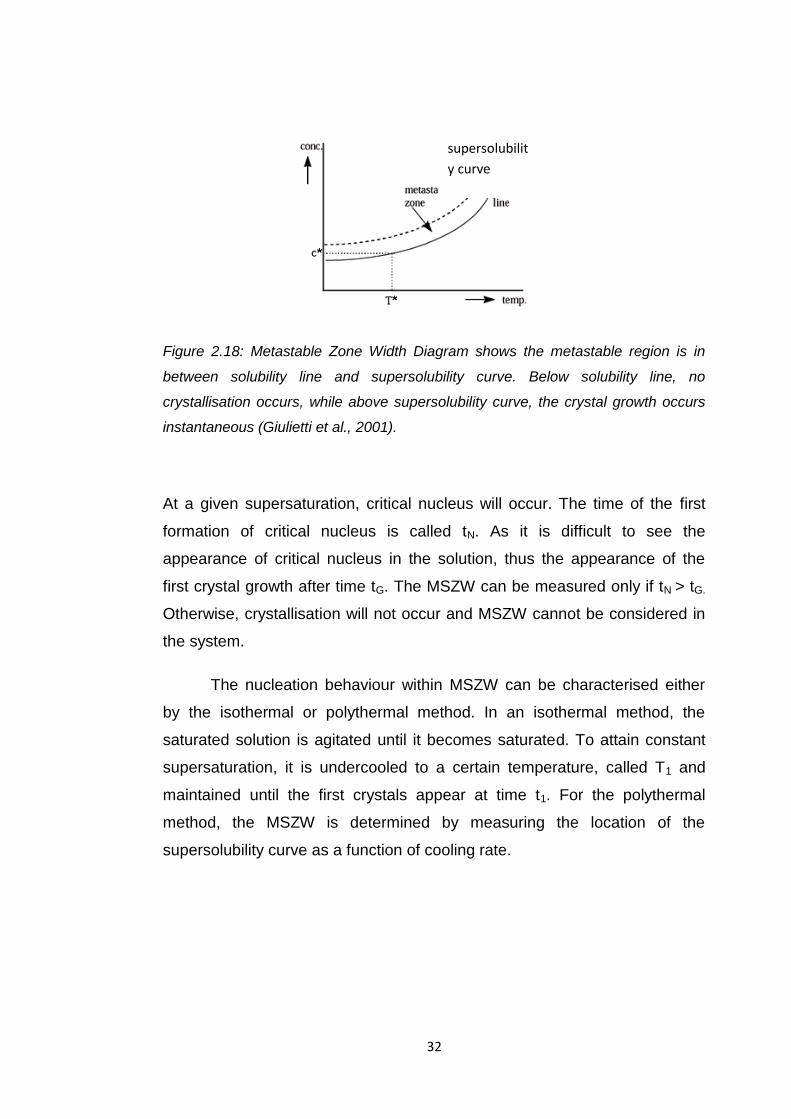
32

Figure 2.18: Metastable Zone Width Diagram shows the metastable region is in

between solubility line and supersolubility curve. Below solubility line, no

crystallisation occurs, while above supersolubility curve, the crystal growth occurs

instantaneous (Giulietti et al., 2001).

At a given supersaturation, critical nucleus will occur. The time of the first

formation of critical nucleus is called tN. As it is difficult to see the

appearance of critical nucleus in the solution, thus the appearance of the

first crystal growth after time tG. The MSZW can be measured only if tN > tG.

Otherwise, crystallisation will not occur and MSZW cannot be considered in

the system.

The nucleation behaviour within MSZW can be characterised either

by the isothermal or polythermal method. In an isothermal method, the

saturated solution is agitated until it becomes saturated. To attain constant

supersaturation, it is undercooled to a certain temperature, called T1 and

maintained until the first crystals appear at time t1. For the polythermal

method, the MSZW is determined by measuring the location of the

supersolubility curve as a function of cooling rate.

supersolubilit

y curve

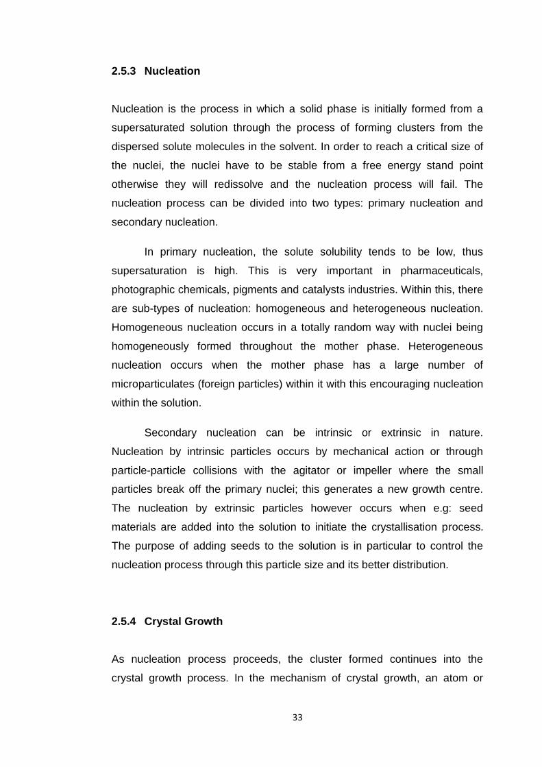
33

2.5.3 Nucleation

Nucleation is the process in which a solid phase is initially formed from a

supersaturated solution through the process of forming clusters from the

dispersed solute molecules in the solvent. In order to reach a critical size of

the nuclei, the nuclei have to be stable from a free energy stand point

otherwise they will redissolve and the nucleation process will fail. The

nucleation process can be divided into two types: primary nucleation and

secondary nucleation.

In primary nucleation, the solute solubility tends to be low, thus

supersaturation is high. This is very important in pharmaceuticals,

photographic chemicals, pigments and catalysts industries. Within this, there

are sub-types of nucleation: homogeneous and heterogeneous nucleation.

Homogeneous nucleation occurs in a totally random way with nuclei being

homogeneously formed throughout the mother phase. Heterogeneous

nucleation occurs when the mother phase has a large number of

microparticulates (foreign particles) within it with this encouraging nucleation

within the solution.

Secondary nucleation can be intrinsic or extrinsic in nature.

Nucleation by intrinsic particles occurs by mechanical action or through

particle-particle collisions with the agitator or impeller where the small

particles break off the primary nuclei; this generates a new growth centre.

The nucleation by extrinsic particles however occurs when e.g: seed

materials are added into the solution to initiate the crystallisation process.

The purpose of adding seeds to the solution is in particular to control the

nucleation process through this particle size and its better distribution.

2.5.4 Crystal Growth

As nucleation process proceeds, the cluster formed continues into the

crystal growth process. In the mechanism of crystal growth, an atom or

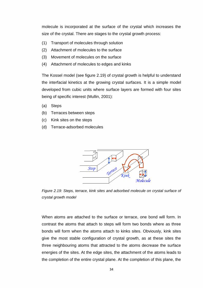
34

molecule is incorporated at the surface of the crystal which increases the

size of the crystal. There are stages to the crystal growth process:

(1) Transport of molecules through solution

(2) Attachment of molecules to the surface

(3) Movement of molecules on the surface

(4) Attachment of molecules to edges and kinks

The Kossel model (see figure 2.19) of crystal growth is helpful to understand

the interfacial kinetics at the growing crystal surfaces. It is a simple model

developed from cubic units where surface layers are formed with four sites

being of specific interest (Mullin, 2001):

(a) Steps

(b) Terraces between steps

(c) Kink sites on the steps

(d) Terrace-adsorbed molecules

Figure 2.19: Steps, terrace, kink sites and adsorbed molecule on crystal surface of

crystal growth model

When atoms are attached to the surface or terrace, one bond will form. In

contrast the atoms that attach to steps will form two bonds where as three

bonds will form when the atoms attach to kinks sites. Obviously, kink sites

give the most stable configuration of crystal growth, as at these sites the

three neighbouring atoms that attracted to the atoms decrease the surface

energies of the sites. At the edge sites, the attachment of the atoms leads to

the completion of the entire crystal plane. At the completion of this plane, the

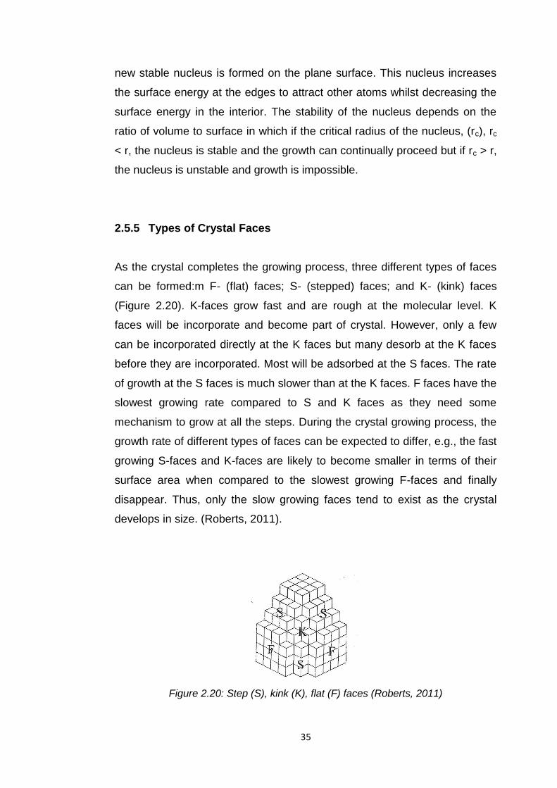
35

new stable nucleus is formed on the plane surface. This nucleus increases

the surface energy at the edges to attract other atoms whilst decreasing the

surface energy in the interior. The stability of the nucleus depends on the

ratio of volume to surface in which if the critical radius of the nucleus, (rc), rc

< r, the nucleus is stable and the growth can continually proceed but if rc > r,

the nucleus is unstable and growth is impossible.

2.5.5 Types of Crystal Faces

As the crystal completes the growing process, three different types of faces

can be formed:m F- (flat) faces; S- (stepped) faces; and K- (kink) faces

(Figure 2.20). K-faces grow fast and are rough at the molecular level. K

faces will be incorporate and become part of crystal. However, only a few

can be incorporated directly at the K faces but many desorb at the K faces

before they are incorporated. Most will be adsorbed at the S faces. The rate

of growth at the S faces is much slower than at the K faces. F faces have the

slowest growing rate compared to S and K faces as they need some

mechanism to grow at all the steps. During the crystal growing process, the

growth rate of different types of faces can be expected to differ, e.g., the fast

growing S-faces and K-faces are likely to become smaller in terms of their

surface area when compared to the slowest growing F-faces and finally

disappear. Thus, only the slow growing faces tend to exist as the crystal

develops in size. (Roberts, 2011).

Figure 2.20: Step (S), kink (K), flat (F) faces (Roberts, 2011)

36

2.6 Agglomeration

Agglomeration is the sticking of particles to one another resulting in the

forming caking through the bridges or lumps. In fine chemical industries for

example in the pharmaceutical industry, agglomeration is desired in order to

improve powder properties i.e, the flowability, compaction behaviour,

increasing the surface area of particles, and reducing the dusting problem

during the handling process (Jeck, 2006). The agglomeration occurs by the

binding mechanism that holds the particles together. Binding occurs by

adhesion forces between particles. These forces determine the strength of

the agglomeration. During agglomeration, new particle sizes form, with

larger sizes than single particle. Agglomerates can be in the form of tablets,

granules, bricks or compaction of particles. The formation of new particle

sizes does not change the original solid particles, size and shape. Jeck,

2006 also explained that agglomeration tends to occur at the fast growing

faces of the crystals.

There are two primary types of agglomerates; (i) soft agglomerates

and (ii) hard agglomerates. The first type of agglomerates may influence the

bulk powder properties as mild forces occur during processing that have a

tendency to break the agglomerates. The latter type normally form larger

size of particles than the primary particles before the agglomeration (Figure

2.21) , thus the breakage can happen if large forces are applied to the

particles such as may take place during the milling process (Nichols, et al.,

2002).

Figure 2.21: Schematic diagram of formation of agglomerates from a group of

particles.

37

In Brunsteiner et al., 2005, a study had been carried out to understand the

agglomeration process at the molecular level by simulating surface

interactions between agglomerates particles. In their study, inorganic and

organic materials had been used to observe the respective differences

between the agglomeration processes for these two types of material. They

discovered that the extent of supersaturation influenced the strength of the

agglomeration.

Using fundamental approaches, the characterisation of particle-particle

interactions forms an important interest in this study. Several methods have

been selected for the characterisation of the agglomerates; surface energy

analysis to determine the average dispersive energy for the batch crystals,

X-ray diffraction to determine the orientation relationship between crystals

and molecular modelling simulation to fully understand the surface chemistry

of the compounds. These methods are described in chapter 3 and 4 of this

thesis.

2.7 Closing Remarks

This chapter has reviewed and discussed the fundamental theories of

crystallography and crystallization process including the basic

crystallography, crystal chemistry and the stages in crystallization process

including nucleation and growth process, mechanism of crystal growth and

morphology of the crystals.

38

References

1. Barret, C., Massalski, T.B., (1980). Structure of Metals. Crystallographic

Methods, Principles and Data In: International Series on Materials

Science and Technology. Third revised ed., vol 35. Pergamon, Oxford.

2. Bragg, W.H., Bragg, W.L., (1913). The Reflection of X-rays by Crystals.

Proc. R. Soc. Lond A: (88) 428-438.

3. Braun, D.E., Gelbrich, T., Kahlenberg, V., Laus, G., Wieser, J.,

Griesser, U.J., (2008). Packing Polymorphism of a Conformationally

Flexible Molecule (Aprepitant). New J. Chem. (32) 1677-1685.

4. Britain, H. G. (1999). Polymorphism in Pharmaceutical Solids. Vol 95.

Marcel Dekker, Inc. New York.

5. Brunsteiner, M., Jones, A.G., Pratola, F., Price, S.L., Simon, S.J.R.,

(2005). Toward A Molecular Understanding of Crystal Agglomeration. J.

Cryst. Growth Des. (5) 3-6.

6. Buckingham, R.A,.(1938). The Classical Equation of State of Gaseous

Helium, Neon, and Argon. Proc. R. Soc. Lond A: Mathematical,

Physical and Engineering Sciences (168) 264-283.

7. Cardew, P.T., (1985). The Growth Shape of Crystals. J. Cryst. Growth.

(73) 385-391.

8. Chen, J., Wang, J., Ulrich, J., Yin, Q., Xue, L., (2008). Effect of Solvent

on the Crystal Structure and Habit of Hydrocortisone. J. Cryst. Growth

Des. (8) 1490-1494.

9. Crystallography. (n.d.) Collins Discovery Encyclopedia, First ed.

(2005).

10. Cramer, C.J., (2002). Essentials of Computational Chemistry: Theories

and Models. First ed. John, Wiley & Sons, England.

11. Curz-Cabeza, A.J., Bernstein, J., (2014). Conformational

Polymorphism. Chem. Rev. (114) 2171-2190.

12. Davey, R., Fila, W., Garside, J., (1986). The Influence of Biuret on the

Growth Kinetics of Urea from Aqueous Solutions. J. Cryst. Growth. (79)

607-613.

39

13. Ferrari, E.S., Davey, R.J., (2004). Solution-mediatied Transformation of

α- to β- L-Glutamic Acid: Rate Enhancement Due to Secondary

Nucleation. J. Cryst. Growth Des. (4) 1061-1068.

14. Giron, D., (2001). Investigations of Polymorphism and Pseudo-

polymorphism in Pharmaceuticals by Combined Thermoanalytical

Techniques. J. Therm. Anal. Cal. (64) 37-60.

15. Giulietti, M., Seckler, M.M., Derenzo, S., Re, M.I., Cekinski, E., (2001).

Industrial Crystallisation and Precipitation from Solutions: States of the

Technique. Brazilian Journal of Chemical Engineering.

16. Glusker, J.P., Trueblood, K.N., (2010). Crystal Structure Analysis. Third

ed. Oxford University Press.

17. Graham, K.R., Stalder, R., Wieruszweski, P.M., Patel, D.G., Salazar,

D.H., Reynolds, J.R., (2013). Tailor-Made Additives for Morphology

Control in Molecular Bulk-Heterojunction Photovoltaics. ACS Appl.

Mater Interfaces. (5) 63-71.

18. Hilfiker, R., (2006). Polymorphism:In the Pharmaceutical Industry.

19. Jeck, S. (2006) Molecular Modeling of Particle-Particle Interactions

Relevant in Understanding Pharmaceutical Formulation Design: A Case

Study of Acetylsalicylic Acid and Ascorbic Acid. Student Exchange

Project Thesis, University of Leeds. Associated paper:

Hammond, R.B., Jeck, S., Ma, C.Y., Pencheva, K., Roberts, K.J.,

Auffret, T., (2009). J. Pharm. Sci. (98) 4589-4602.

20. Ladd, M.F.C., (1979). Structure and Bonding in Solid State Chemistry.

(Ellis Horwood Series in Chemical Science). Ellis Horwood Ltd, New

York.

21. Kelly, A., Knowles, K.M., (2012). Crystallograhy and Crystal Defects.

Second ed. John Wiley & Sons, Ltd, Chichester, UK.

22. Milburn, G.H.W., (1973). X-ray Crystallography. First Ed. Butterworths

and Co. Ltd., London.

23. Mirmehrabi, M., Rohani, S., (2006). Polymorphic Behaviour and Crystal

Habit of an Anti-Viral/ HIV Drug: Stavudine. J. Cryst. Growth Des. (6)

14-149.

24. Mullin, J.W., (2001). Crystallisation. Fourth ed. Butterworth-Heinemann,

Oxford.

40

25. Nichols, G., Byard, S., Bloxham, M.J., Botterill, J., Dawson, N.J.,

Dennis, A., Diart, V., North, N.C., Sherwood, J.D., (2002). A Review of

the Terms Agglomerate and Aggregate with Recommendation for

Nomenclature Used in Powder and Particle Characterisation. J. Pharm.

Sci., (91) 10.

26. Oobatake, M., Ooi, T., (1972). Determination of Energy Parameters in

Lennard-Jones Potentials from Second Virial Coefficients. Prog. Of

Theoretical Physics.(48) 2132-2143.

27. Phillips, F.C., (1963). An Introduction to Crystallography. Third ed.

Longmans, Green and Co. Ltd, London.

28. Redinha, J.S., Jesus, .A.J.L., Pais, A.A.C.C., Almeida, J.A.S., (2013).

Crystallisation: From the Conformer to the Crystal. Book Article:

Advanced Topics on Crystal Growth. Dr. Sukarno Ferreira (Ed.)

29. Roberts, K.J., (2011). Pharmaceutical Product Formulation.

PEME5360M Course Notes, School of Process, Environmental and

Materials Engineering, University of Leeds.

30. Roberts, K.J., Sherwood, J.N., Yoon, C.S., (1994). Understanding the

the Solvent-Induced Habit Modification on Benzophenone in Terms of

Molecular Recognition at the Crystal / Solution Interface. Chem. Mater.

(6) 1099-1102.

31. Watanabe, A., Yamaoka, Y., Kozo, T., (1982). Crystal Habits and

Dissolution Behaviour of Aspirin. Chem. Pharm. Bull. 30 (8) 2958-2963.

41

CHAPTER III

SURFACE AND SOLID-STATE ANALYSIS AND

CHARACTERISATION OF MICRO-CRYSTALS

42

3.1 Introduction

This chapter discusses the theoretical background to the solid-state and

surface characterisation techniques used in this work. It includes the

investigation of surface energy analysis of solid particles conducted by

inverse gas chromatography (IGC), the use of dynamic vapour sorption

(DVS) for characterisation of water sorption effect to the surface of solid

particles, the measurement of the size and shape of the crystals and the

technology of synchrotron radiation for the measurement of the crystal

structure, crystal aggregation and 3-D morphology use in X-ray micro-

diffraction and X-ray micro-tomography techniques.

3.2 Surface Analysis Techniques

3.2.1 Inverse Gas Chromatography (IGC) For Surface Energy Analysis

The determination of the surface free energy in particles processing is very

important in order to determine the stability, adhesion and cohesion between

particles and also the interactions among the molecules in the crystal

packing. These properties are important to understand to ensure the final

products meet their specification. The results from surface characterisation

of solid particles help the related industries to improve the surface properties

and whether to do some modifications to increase product performance. It

also helps to fundamentally understand the surface chemistry of the

particles. Surface free energy characterisation is important in pharmaceutical

dosage and pharmaceutical processing and to help determine the granule

strength, morphology, failure process, and the formation of film on the

binders (Hooton et al., 2006).

In surface energetic studies, the interactions between solid surfaces

and the external environment occur due to the termination of the bulk crystal

structure at the crystal surfaces with the resultant surface energies reflecting

the nature and strength of the ‘broken bond’ component of the existence of

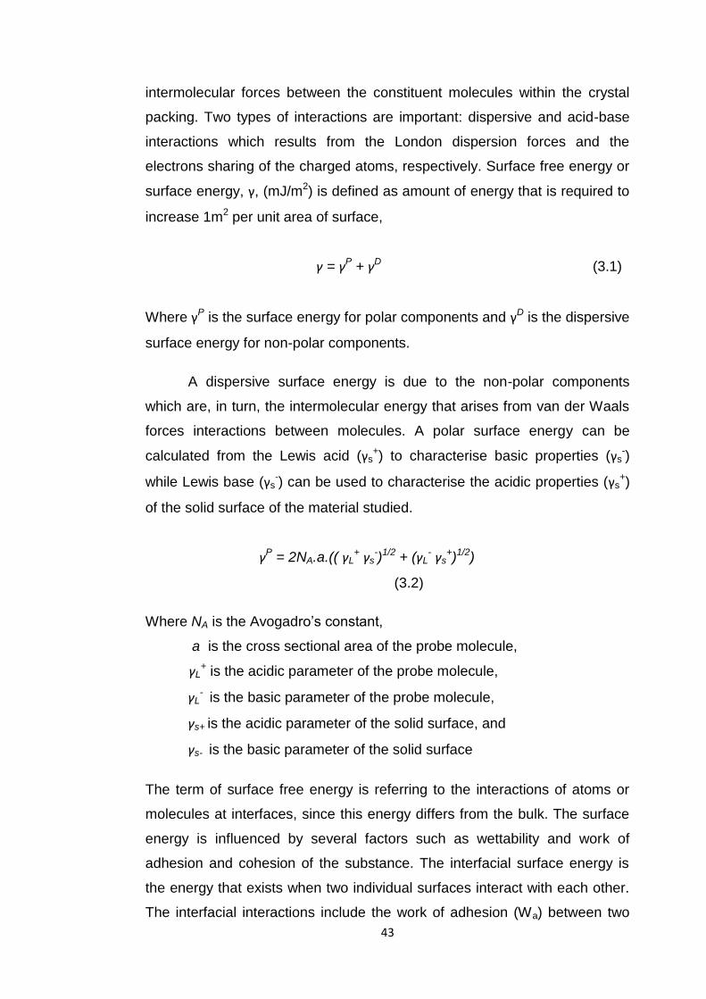
43

intermolecular forces between the constituent molecules within the crystal

packing. Two types of interactions are important: dispersive and acid-base

interactions which results from the London dispersion forces and the

electrons sharing of the charged atoms, respectively. Surface free energy or

surface energy, γ, (mJ/m2) is defined as amount of energy that is required to

increase 1m2 per unit area of surface,

γ = γP + γD (3.1)

Where γP is the surface energy for polar components and γD is the dispersive

surface energy for non-polar components.

A dispersive surface energy is due to the non-polar components

which are, in turn, the intermolecular energy that arises from van der Waals

forces interactions between molecules. A polar surface energy can be

calculated from the Lewis acid (γs+) to characterise basic properties (γs

-)

while Lewis base (γs-) can be used to characterise the acidic properties (γs

+)

of the solid surface of the material studied.

γP = 2NA.a.(( γL+ γs

-)1/2 + (γL- γs

+)1/2)

(3.2)

Where NA is the Avogadro’s constant,

a is the cross sectional area of the probe molecule,

γL+ is the acidic parameter of the probe molecule,

γL- is the basic parameter of the probe molecule,

γs+ is the acidic parameter of the solid surface, and

γs- is the basic parameter of the solid surface

The term of surface free energy is referring to the interactions of atoms or

molecules at interfaces, since this energy differs from the bulk. The surface

energy is influenced by several factors such as wettability and work of

adhesion and cohesion of the substance. The interfacial surface energy is

the energy that exists when two individual surfaces interact with each other.

The interfacial interactions include the work of adhesion (Wa) between two

44

phases and work of cohesion (Wc) of one phase. The subtraction of the work

of adhesion from the work of cohesion gives the value for the spreading

coefficient, λ, which is an important parameter in determining the granule

strength. A positive value of the spreading coefficient is indicative of strong

granules whilst a negative value is more consistent of weak granules (Rowe,

1989a), thus:

λ = Wa – Wc (3.3)

In the earlier studies of the surface energetic nature of solid particles,

contact angle measurements were a popular method in determining the

surface energy of the solid. The contact angle between liquid and solid is

measured by dropping a small drop of liquid on the solid surface and

measuring the interaction between the liquid and solid by using Young’s

equation (Zisman, 1964). There are several methods that have used contact

angle techniques to measure the surface energy of the solid, including the

sessile drop method (Nizhenko et al., 1964), Wilhelmy method (Heertjes et

al., 1971), and powder contact angle method using a static capillary rise

technique (Dunstan & White, 1986). However, the results obtained from

contact angle techniques can be affected by the compression of the powder

on the disk in which the compression may change the surface properties,

affecting the accuracy of the measurement (Grimsey et al., 2002). In the

early 1970s, inverse gas chromatography (IGC) had been introduced for

surface energy determination. In 1989, this technique had been used to

study the water binding on egg solid (Demertzis & Kontominas, 1989). Dove

et al., 1996 did a comparison study between contact angle techniques and

inverse gas chromatography. The two methods of contact angle

measurement used were compressing a plate of powder and sticking

uncompressed powder on the plate. From this investigation, they found that

the inverse gas chromatography technique gave similar values to the contact

angle measurement techniques. The first authors to introduce inverse gas

chromatography method in pharmaceutical field were Huu-Phouc et al., in

1986 in who used IGC to determine the partial solubility parameters of

lactose.

45

The surface energy of powder materials can also be determined by

IGC. Generally, IGC determines the thermodynamic parameters of the

solids, specifically the partition and solubility coefficients, enthalpies of

adsorption, free energy of adsorption and also the sorption isotherms of the

adsorbate. The utility of IGC in measuring the surface properties of the

materials have made it very useful in the pharmaceutical, food, dying or

painting industries. In the food industry, for example, the thermodynamic

properties of aromatic-starch interactions (Boutboul et.al, 2002) have been

determined. In other studies, the polar and total surface energy distributions

of lactose from the known dispersive surface energy has been obtained from

the IGC calculation (Das et al., 2011).

In IGC, the solid material is packed in a long, thin packed column

which acts as an adsorbent and is a stationary phase while the volatile

probes pass through the column as the adsorbate. To determine the

dispersive surface energy, a series of n-alkanes can be used as non-polar

solutes while polar probes such as alcoholic solvents to study the acid-base

interactions of the solid particles for polar surface energy determination. The

probe residence time, tr (min) can be calculated as the probes passed

through the column and hence the shape of the resultant chromatogram

indicate the characteristics of the stationary phase and its interaction with

the probes. From the residence time, the net retention volume, VN can be

calculated by using the equation 3.4:

VN = Fc.J (tr – to) (3.4)

From the net retention volume, the specific retention volume can be obtained

from the following equation 3.5:

(3.5)

Where,

Fc is the carrier gas flow rate, ml/min,

to is the hold-up time of non-retained compound (methane), min,

46

m is the mass of stationary phase, g,

T is the temperature of the column, K, and

J is the correction factor for the compressibility of the carrier gas.

J can be obtained from the equation 3.6 below:

(3.6)

where, Pi and Po are inlet and outlet pressures respectively.

In IGC, there are two methods of dispersive surface energy

calculation have been commonly used are Dorris-Gray and Schultz

methods. Different values had been obtained, with the larger value coming

from the Doris-Gray method compared to Schultz method (Shi et al., 2002).

The dispersive surface energy can be calculated from the adsorption free

energy of the probes, ∆Gads which can be calculated by the following

equation 3.7. Thus:

∆Gads = -RT. ln VN + C (3.7)

where, R is a universal gas constant, T is the temperature of the column, VN

is a net retention volume of the n-alkane probes with the carbon number, n,

and C is a constant, depending on the reference state absorption.

Injection of polar probes into the column causes an interaction between

dispersive and special interaction of molecules probes with the solid

samples in the column. Thus, ∆Gads is given by equation 2.8:

∆Gads = ∆GDP + ∆GSP (3.8)

Where ∆GDP is a dispersive interactions while ∆GSP is a special interactions.

The dispersive surface energy is calculated by using Fowkes equation which

takes into consideration the work of adhesion and the dispersive component

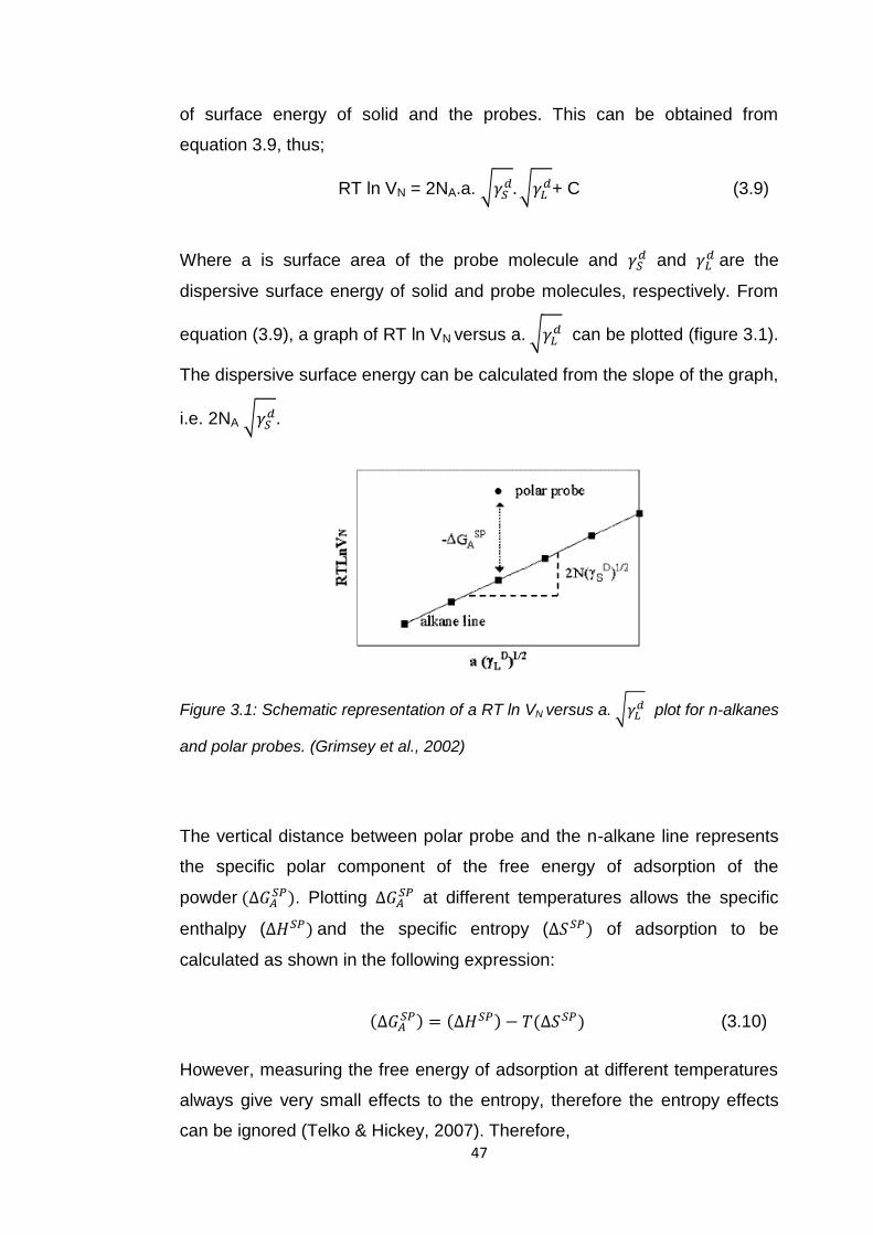
47

of surface energy of solid and the probes. This can be obtained from

equation 3.9, thus;

RT ln VN = 2NA.a.

+ C (3.9)

Where a is surface area of the probe molecule and and

are the

dispersive surface energy of solid and probe molecules, respectively. From

equation (3.9), a graph of RT ln VN versus a. can be plotted (figure 3.1).

The dispersive surface energy can be calculated from the slope of the graph,

i.e. 2NA .

Figure 3.1: Schematic representation of a RT ln VN versus a. plot for n-alkanes

and polar probes. (Grimsey et al., 2002)

The vertical distance between polar probe and the n-alkane line represents

the specific polar component of the free energy of adsorption of the

powder . Plotting

at different temperatures allows the specific

enthalpy ( and the specific entropy ( of adsorption to be

calculated as shown in the following expression:

(3.10)

However, measuring the free energy of adsorption at different temperatures

always give very small effects to the entropy, therefore the entropy effects

can be ignored (Telko & Hickey, 2007). Therefore,

48

(3.11)

Acid-base properties of the surface energy of solid particles can be obtained

by using Gutmann’s equation (Comte, et al., 2005), thus:

(3.12)

Where ∆G is the specific interaction adsorption surface energy of solid

particle,

KA is the acidity value of solid particle,

KB is the basicity value of solid particle,

AN* is the acceptor number, and

DN is the donor number

The determination of acid-base properties in the surface energy

determination is important to understand the surface properties of particles.

The interaction of electron acceptors and donors (Lewis acid-base) gives

information on the acidity and basicity of the solid particles (Panzer and

Schreiber, 1992, Donnet et al., 1991). Furthermore, the calculation of

surface energy and acid-base interactions of particles, determines the

surface thermodynamic properties of solid particles (Chehimi et al., 1995).

From previous studies it is now known that the morphology of the substrate

materials has a significant effect on the surface energy determination of the

crystal. Storey carried out experimental work using several ibuprofen

crystals that were recrystallised in different solvents; hexane, acetonitrile and

methanol which produced different shaped crystals. This, in turn, was found

to change the dispersive surface energy due to the different intermolecular

interactions involved for the different surface chemistries of the crystal habit

faces (Storey, 1997). The IGC has also been used for thermal analysis and

has been shown to give highly accurate results as it has been found to be

very sensitive to changes in the relative humidity of the probe vapours.

These changes of relative humidity have been changed the surface energy

49

of solid particles. As the relative humidity increased, the surface energies

were found to decrease. This is was found to be consistent with the

adsorbed water molecules competing for the same sites as the probes

decreasing their interaction with the surface (Sunkersett et al., 2001). To

demonstrate that IGC gives the accurate vapour sorption results, a

comparison study between isothermal microcalorimetry and IGC was carried

out (Buckton et al., 1999). In this, three samples of saquinavir mesylate an

anti-viral drug at different drying conditions was used to determine the

dispersive surface energies and the water sorption of the samples. As both

methods were found to be highly accurate in terms of measuring the

changes between samples that IGC can be as good as isothermal

calorimetry in terms of its sensitivity even when small changes in the sample

occurred.

3.2.2 Dynamic Vapour Sorption

Besides IGC, this work showed an alternative approach to study the sorption

isotherm for solid particles is dynamic vapour sorption (DVS). DVS has been

developed from gravimetric techniques and measures how much a sample

adsorbs and desorbs water vapour. In a similar to IGC, DVS is also widely

used in fine and a powder industry due to the very sensitive measurements it

provides only requires 1-100 mg of sample. Sorption isotherm analysis is

mainly used to characterise solid-vapor interactions. It measures the vapour

absorbed or desorbed to and from the samples as a function of vapour

pressure (Smith et al., 2004). In water sorption analysis, three methods have

been used; (i) the weighing bottle and salt solution method, (ii) the

gravimetric method, (iii) the volumetric method (McLaren & Rowen, 1951).

The weighing bottle and salt solution method is the oldest technique.

However, the sensitivity of this technique is low and it can take a long time to

reach the equilibrium state because of the gases interference in the system

and the associated inaccuracies that need to be eliminated. In DVS, the

gravimetric method is used in which a high sensitive microbalance is used to

50

weigh the sample. Because of high sensitivity, it gives high accuracy and

also gives rapid results (Williams & Levoguer, 2006). This technique is

widely used in the polymer, food, pharmaceutical, building materials

industries etc. In pharmaceutical processing, it is very important to measure

the water sorption isotherms of the powders because of the concern of

bioavailability of the pharmaceutical products when administered to the

human body and also their tendency to changes in their polymorphic form

during the storage. For example, after the spray drying process in drugs

formulation, the stability of the products in absorbing water must be

observed (Tzannis and Prestrelski, 1998). During the processing of

pharmaceutical solids, the amorphous materials may be produced which will

affect the products stability and producibility. This is because amorphous

materials are highly unstable due to the random arrangement of molecules.

Thus, DVS can also be used to determine the amorphous content in the

drugs powder (Mackin et al., 2002), (Columbano et al., 2002). In amorphous

materials the glass transition temperature, Tg, is important which is the

starting temperature for crystalline materials to change to the amorphous

state or vice versa. Thus, it is important to know the Tg for pharmaceutical

compounds that easily transform in amorphous form state. Such a study had

been carried out on amorphous lactose to determine its Tg, thus enabling the

effective control over the crystallization process to prevent the formation of

the amorphous phase (Buckton & Darcy, 1996).

3.3 X-ray Techniques

3.3.1 X-Ray Diffraction

X-ray diffraction (XRD) is a technique to determine the structure of the

matter. It gives information on molecular packing in the unit cell, coordinates

of each atom and intermolecular interactions. Including this information, the

orientation of the crystal can also be determined using this technique. As in

real crystal products, most of the crystals have defects, thus, by using XRD,

defects in crystal can also be characterised. It can also determine whether

51

the solid is in the crystal or amorphous form. There are two types of popular

XRD techniques that have been used, powder XRD and single crystal XRD.

In powder XRD, powdered sample is used, with a large number of

crystallites. An X-ray beam is impinged on the powder sample, which will

diffract and produce diffraction planes with different angles depend on the

crystal orientation, size and strain. As the particle size decreases, the peak

width becomes larger due to the decrease in destructive interference close

to the Bragg angles associated with the increase in surface to bulk ratio of

the particle. Powder XRD can also be used to determine the existence of

polymorphs within a sample. Each polymorph has a different crystal

structure with different atomic positions, size and shape, thus, the diffraction

patterns of each will be different. However, the result of powder XRD is not

as precise as in single crystal XRD, where it is possible to obtain more

structural detail including bond lengths and angles. In a similar manner to

powder XRD, in single crystal XRD, the X-ray beams is impinged on the

sample, however, in this case, only one single crystal would be used for

examination by the beam with the sample being rotated to select different

crystal planes for diffraction.

In XRD, electromagnetic radiation waves are used. The

electromagnetic radiation accelerates in a vacuum very close with the

velocity of light. The energy produced by the moving charged particles or

electrons are called photons in an electric field, E. The vectors electric field

and magnetic field, H, are both orthogonal to the direction of wave

propagation (figure 3.2). As the wave is incident on the atoms in the crystal

lattice, it scatters the X-ray waves in all directions. As a result, the X-ray

waves give a diffraction pattern dependent on the crystal structure and

interplanar spacing, d, of the lattice. The interplanar spacing is dependent on

the lattice parameters, a, b, and c of the unit cell. The electromagnetic

radiation is measured by energy, E, wavelength, λ or frequency, . All these

parameters are related each other in the equation 3.13 and 3.14:

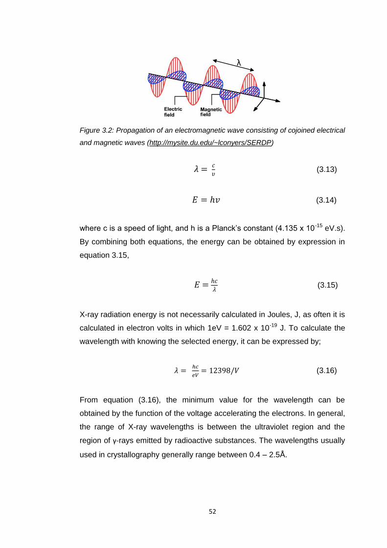
52

Figure 3.2: Propagation of an electromagnetic wave consisting of cojoined electrical

and magnetic waves (http://mysite.du.edu/~lconyers/SERDP)

(3.13)

(3.14)

where c is a speed of light, and h is a Planck’s constant (4.135 x 10-15 eV.s).

By combining both equations, the energy can be obtained by expression in

equation 3.15,

(3.15)

X-ray radiation energy is not necessarily calculated in Joules, J, as often it is

calculated in electron volts in which 1eV = 1.602 x 10-19 J. To calculate the

wavelength with knowing the selected energy, it can be expressed by;

(3.16)

From equation (3.16), the minimum value for the wavelength can be

obtained by the function of the voltage accelerating the electrons. In general,

the range of X-ray wavelengths is between the ultraviolet region and the

region of γ-rays emitted by radioactive substances. The wavelengths usually

used in crystallography generally range between 0.4 – 2.5Å.

λ

http://mysite.du.edu/~lconyers/SERDP

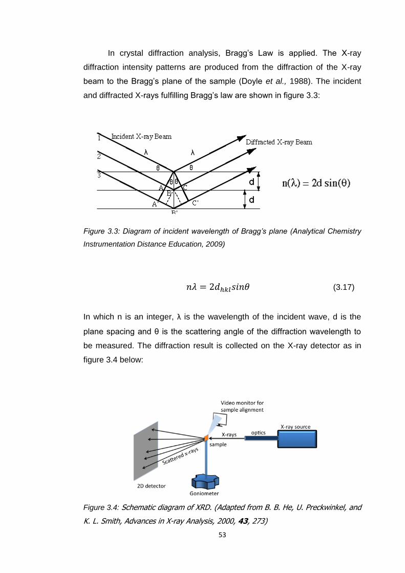
53

In crystal diffraction analysis, Bragg’s Law is applied. The X-ray

diffraction intensity patterns are produced from the diffraction of the X-ray

beam to the Bragg’s plane of the sample (Doyle et al., 1988). The incident

and diffracted X-rays fulfilling Bragg’s law are shown in figure 3.3:

Figure 3.3: Diagram of incident wavelength of Bragg’s plane (Analytical Chemistry

Instrumentation Distance Education, 2009)

(3.17)

In which n is an integer, λ is the wavelength of the incident wave, d is the

plane spacing and θ is the scattering angle of the diffraction wavelength to

be measured. The diffraction result is collected on the X-ray detector as in

figure 3.4 below:

Figure 3.4: Schematic diagram of XRD. (Adapted from B. B. He, U. Preckwinkel, and

K. L. Smith, Advances in X-ray Analysis, 2000, 43, 273)

λ λ

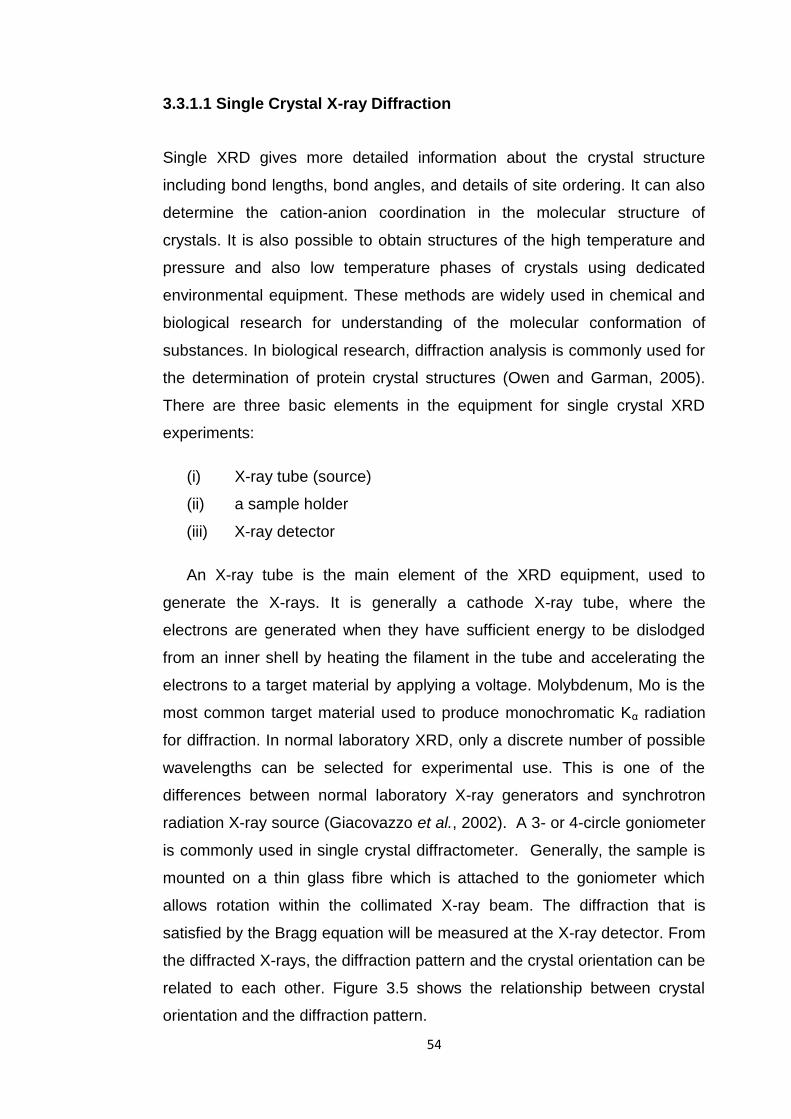
54

3.3.1.1 Single Crystal X-ray Diffraction

Single XRD gives more detailed information about the crystal structure

including bond lengths, bond angles, and details of site ordering. It can also

determine the cation-anion coordination in the molecular structure of

crystals. It is also possible to obtain structures of the high temperature and

pressure and also low temperature phases of crystals using dedicated

environmental equipment. These methods are widely used in chemical and

biological research for understanding of the molecular conformation of

substances. In biological research, diffraction analysis is commonly used for

the determination of protein crystal structures (Owen and Garman, 2005).

There are three basic elements in the equipment for single crystal XRD

experiments:

(i) X-ray tube (source)

(ii) a sample holder

(iii) X-ray detector

An X-ray tube is the main element of the XRD equipment, used to

generate the X-rays. It is generally a cathode X-ray tube, where the

electrons are generated when they have sufficient energy to be dislodged

from an inner shell by heating the filament in the tube and accelerating the

electrons to a target material by applying a voltage. Molybdenum, Mo is the

most common target material used to produce monochromatic Kα radiation

for diffraction. In normal laboratory XRD, only a discrete number of possible

wavelengths can be selected for experimental use. This is one of the

differences between normal laboratory X-ray generators and synchrotron

radiation X-ray source (Giacovazzo et al., 2002). A 3- or 4-circle goniometer

is commonly used in single crystal diffractometer. Generally, the sample is

mounted on a thin glass fibre which is attached to the goniometer which

allows rotation within the collimated X-ray beam. The diffraction that is

satisfied by the Bragg equation will be measured at the X-ray detector. From

the diffracted X-rays, the diffraction pattern and the crystal orientation can be

related to each other. Figure 3.5 shows the relationship between crystal

orientation and the diffraction pattern.

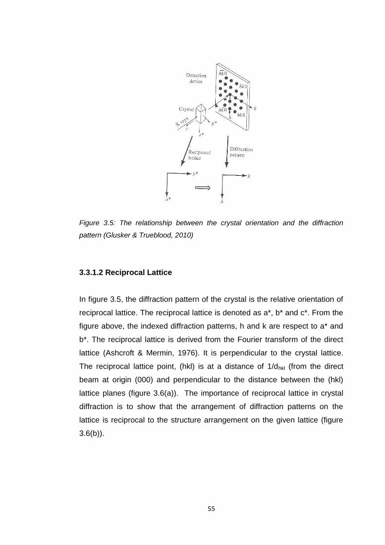
55

Figure 3.5: The relationship between the crystal orientation and the diffraction

pattern (Glusker & Trueblood, 2010)

3.3.1.2 Reciprocal Lattice

In figure 3.5, the diffraction pattern of the crystal is the relative orientation of

reciprocal lattice. The reciprocal lattice is denoted as a*, b* and c*. From the

figure above, the indexed diffraction patterns, h and k are respect to a* and

b*. The reciprocal lattice is derived from the Fourier transform of the direct

lattice (Ashcroft & Mermin, 1976). It is perpendicular to the crystal lattice.

The reciprocal lattice point, (hkl) is at a distance of 1/dhkl (from the direct

beam at origin (000) and perpendicular to the distance between the (hkl)

lattice planes (figure 3.6(a)). The importance of reciprocal lattice in crystal

diffraction is to show that the arrangement of diffraction patterns on the

lattice is reciprocal to the structure arrangement on the given lattice (figure

3.6(b)).

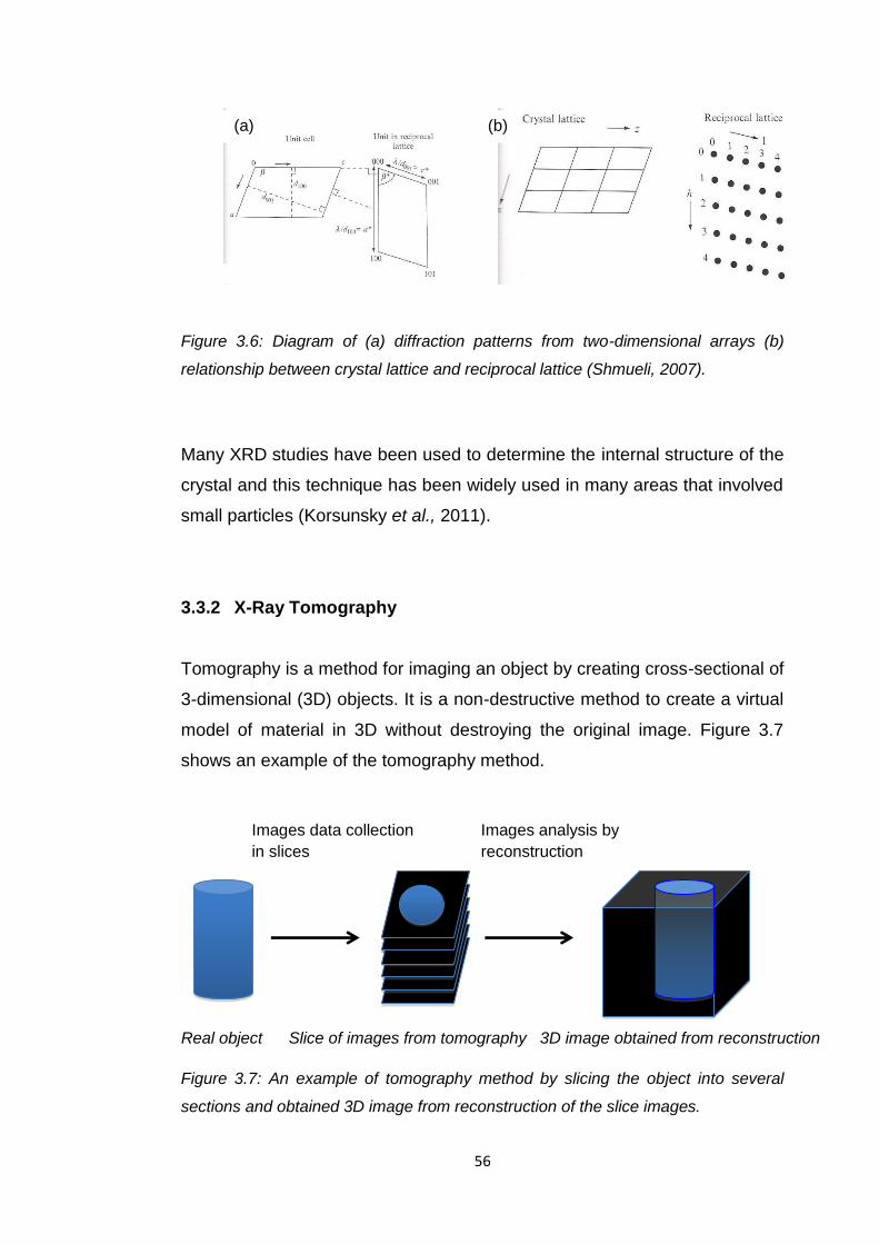
56

Figure 3.6: Diagram of (a) diffraction patterns from two-dimensional arrays (b)

relationship between crystal lattice and reciprocal lattice (Shmueli, 2007).

Many XRD studies have been used to determine the internal structure of the

crystal and this technique has been widely used in many areas that involved

small particles (Korsunsky et al., 2011).

3.3.2 X-Ray Tomography

Tomography is a method for imaging an object by creating cross-sectional of

3-dimensional (3D) objects. It is a non-destructive method to create a virtual

model of material in 3D without destroying the original image. Figure 3.7

shows an example of the tomography method.

Figure 3.7: An example of tomography method by slicing the object into several

sections and obtained 3D image from reconstruction of the slice images.

(a) (b)

Real object Slice of images from tomography 3D image obtained from reconstruction

Images data collection

in slices

Images analysis by

reconstruction

57

This technique is widely used in medicine as a computed-tomography (CT)

scan for bone imaging, tumour imaging and infant imaging (Davis & Wong,

1996, Beckman et al., 1999). It is also used in geology to determine the

porosity of the soil, space study of meteorites (Ebel & Rivers, 2007), food

industries, and electronic industries. The advantage of this technique is that

it is possible for the high intensity of the light to penetrate the dense objects.

The effect of cracks and voids in carbon/carbon composites which are used

in the aerospace industry also use X-ray tomography (XMT) to visualise the

microcracking in the samples (Paris et al., 2001). The images that are

obtained from the projection of the light will be reconstructed using

algorithms to get a clear or structural shape of the particles. Some software

can be used for the image analysis. ImageJ is used to define the region of

interest of the images obtained from the raw data (Collin, 2007), filter and

threshold for reducing noise and determine a pixel and produce the binary

image. The image analysis can be carried out by mathematical analysis,

Landis & Keane, (2010) reviewed these analytical methods. In tomographic

reconstruction mathematics, the information is obtained from two-

dimensional absorption of light images and it is reconstructed to produce a

three-dimensional digital image. The absorption of light is an algorithmic

function of how the materials absorbed the light and the distance through

which the light must travel.

3.3.3 Synchrotron Radiation

Synchrotron radiation (SR) is a technique that generates high

electromagnetic radiation energy (Ivanenko & Pomeranchuck, 1944) by

accelerating electrons that are moving along a bending magnetic field that

causes the electron beam to travel in a circular path. Synchrotron light is one

type of Radio Frequency (RF) accelerator, in which the electric field is not

static but oscillates at some frequency. The first discovery of synchrotron

light occurred from the experimental observation that the light observed from

70MeV with a small spot but bright light visibly can be seen from the output

machine (Elder et al., 1947).

58

3.3.3.1 Development of Synchrotron Radiation Source

First Generation of Storage Rings

In the earliest development of synchrotron radiation, the first generation of

synchrotron radiation sources was a development of electron storage rings,

which is an important part of the synchrotron radiation source because the

electrons accelerate in this medium (Bilderback et al., 2005). However, in

the earliest work, it was operated in a parasitic mode, primarily for high

energy physics research. The first major development of storage rings to be

dedicated to synchrotron radiation was developed at the University of

Wisconsin called Tantalus I, with 3.45 m diameter of storage ring, 8 bending

magnets had been used, producing 240MeV electron energy with 10

beamlines. This enabled some of the early pioneering research into

synchrotron radiation studies to be carried out. The synchrotron beam

circulated continuously with repeated sequences of injection, acceleration,

and extraction up to 50 Hz. The synchrotron radiation source provided high

flux, high beam stability and a reduced radiation hazard (Rowe & Mills,

1973).

Second Generation of Storage Rings

In the second generation storage rings, dedicated synchrotron sources were

designed and were used in various applications. Large numbers of

beamlines and experimental stations has been produced to serve many

users. However, bending magnets were still the main source of electron

beam acceleration the electrons for producing the SR light.

Third Generation of Storage Rings

In synchrotron radiation light sources, the high flux alone was not felt to be

sufficient as many synchrotron radiation studies relied on the brightness of

the light. The brightness is defined as (3.18),

59

(3.18)

To achieve high brightness, a large number of photons need to be produced

in a given time and small area. A small area is produced by little beam

divergence, and the photon energies also have to be concentrated.

Therefore, to increase the brightness, the vertical slits are required to narrow

the angular divergence; hence a smaller beam size is produced. A small

beam size is necessary in a crystallography experiment when a sample of

small crystals is used. It is beneficial to have a matching incident beam to

the crystal size, whilst still maintaining the angular resolution for diffracted

spots because it maximises the signal to noise ratio. Many developments

had occurred from time to time to improve the light sources to ensure they

give a high performance. The major improvement that had been done in

third generation sources to achieve high brightness was by using insertion

devices. These insertion devices are placed at the empty straight sections

between the bending magnets in the storage rings. Along the trajectory path,

insertion devices are placed that are arrays of magnets such as “undulators”

and “wigglers” to produce the wiggling movement of electrons along the path

that gives highly intense and tunable light. The insertion devices create a

sinusoidal magnetic field, to force the particles to oscillate around the mean

orbit. The light circulating the ring then travels into the beam lines in which

the experiments are carried out. The wavelength of the synchrotron light that

pass into the beam lines differ depending on the application and the

requirements of the experiments. The tunable wavelengths allow the use of

ultraviolet waves or soft or hard X-rays depending on the experiments to be

carried out. Third generation synchrotrons have achieved a mature stage in

which the high brightness and intensities of light have been produced

effectively (Winick, 1998).

60

3.3.3.2 Overview of Synchrotron Radiation Source

Figure 3.8: Schematic diagram of Synchrotron Radiation ring at Diamond Light

Source.

In this thesis work the Diamond Light Source (DLS) was used to carry

out the XRD experiments. Figure 3.8 shows the schematic diagram of the

synchrotron ring at DLS. The main elements of synchrotron radiation

facilities are the electron gun, linear accelerator, booster synchrotron, and

synchrotron ring itself. The ring is not truly in a circular shape, but it is

actually a multi-sided polygon. The electrons are generated in the electron

gun, in which the electrons are produced using a high voltage cathode under

vacuum then accelerated to about 90keV. The electrons are further

accelerated using the first particle accelerator, the Linac to give extremely

high energy at about 100MeV using radio frequency (RF) cavities. The

second particle accelerator called the booster synchrotron helps the

electrons to move in a circular track in which bending magnets are inserted

to bend the electrons to ensure they move in right path. Here, the electrons

are accelerated further to achieve of 3 GeV. The charged particles moving

along a circular orbit emit electromagnetic radiation. The parameter of

61

interest to compare with different synchrotron source is the source size,

which is how effective cross-section of the emitting particle beam, the beam,

the beam emittance which is a constant along the particle path, and the

divergence of the emitted X-ray beam (Giacovazzo, et al., 2002). These

beam lines guide the beams of light to the experimental stations. Each beam

lines have 3 main parts:

(1) Optics hutch

(2) Experimental lab

(3) Control cabin

In the optics hutch, the X-ray beam from the storage ring has the relevant

energy selected and is then focused in this section towards the sample. The

sample is placed in the experimental hutch on the goniometer, in which the

beam interacts with the sample. The control cabin is the room where the

experiments are controlled via computers that are connected to the

equipment where data is collected from the experiment. There are many

uses of synchrotron radiation. The beam lines support experiments such as

diffraction, imaging and spectroscopy with different wavelengths depending

on the type of experiments that are carried out. Synchrotron radiation single

crystal XRD has been widely used in many areas to determine the crystal

structures and confirmation of the lattice parameters such as in the

mineralogy processing industry (Pluth et al., 1997), in biology to find

complex protein crystal structures (Cusack et al., 1998) and also in the

pharmaceutical industry to determine the small molecules of pharmaceutical

drug crystals (Sharff and Jhoti, 2003). In the pharmaceutical industry, the

determination of the shape of the particles using X-ray tomography has

become a major interest to be studied since it is important to understand the

effect of surface/surface interactions between particles on the performance

of the powder after it has processed.

62

3.4 Closing Remarks

This chapter has described about the theoretical principles of the methods

used in this research including the surface characterization using IGC, DVS,

X-ray diffraction and tomography, and the technology of synchrotron

radiation.

References

1. Analytical Chemistry Instrumentation Distance Education, Chemical

Instrumentation Facility, Depatrment of Chemistry, IOWA State

University,(2009):http://www.acide.chem.iastate.edu/xrd/high%20sch

ool/xrd012006.htm

2. Ashcroft, N.W., Mermin, N.D., (1976). Solid State Physics. Holt,

Rinehart and Winston, New York.

3. Beckman, F. Heise, K., Kolsch, B., Bonse, U., Rajewsky, M.F.,

Bartscher, M., Biermann, T., (1999). Three-dimensional of Nerve

Tissue by X-ray Phase-Contrast Microtomography. Biophys. J. (76)

98-102.

4. Bilderback, D.H., Elleaume, P., Weckert, E., (2005). Review of Third

and Next Generation Synchrotron Light Sources. J. Phys. B: At. Mol.

Opt. Phys. (38) S773-S797.

5. Boutboul, A., Lenfant, F., Giampaoli, P., Feigenbaum, A., Ducruet, V.,

(2002). Use of Inverse Gas Chromatography to Determine

Thermodynamic Parameters of Aroma-Starch Interactions. J.

Chromatogr A. (969) 9-16.

6. Buckton, G., Darcy, P., (1996). Water Mobility in Amorphous Lactose

below and Close to the Glass Transition Temperature. Int. J. Pharm.

(136) 141-146.

http://www.acide.chem.iastate.edu/xrd/high%20school/xrd012006.htm

http://www.acide.chem.iastate.edu/xrd/high%20school/xrd012006.htm

63

7. Buckton, G., Dove, J.W., Davies, P., (1999). Isothermal

Microcalorimetry and Inverse Gas Chromatography to Study Small

Changes in Powder Surface Properties. Int. J. Pharm. (193) 13-19.

8. Chehimi, M., Lascelles, S., Armes, P., (1995). Characterisation of

Surface Thermodynamic Properties of p-Toluene Sulfonate-doped

Polypyrrole by Inverse Gas Chromatography. Chromatographia. (41)

671-677.

9. Collin, T.J, 2007. Image for Microscopy. BioTechniques. 43, 25-30.

10. Columbano, A., Buckton, G., Wikeley, P., (2002). A Study of the

Crystallisation of Amorphous Salbutamol.Sulphate using Water

Wapour Sorption and Near Infrared Spectroscopy. Int. J. Pharm.

(237) 71-178.

11. Comte, S., Calvet, R., Dodds, J.A., Balard, H., (2005). Surface

Properties of Low Specific Surfce Powders using Inverse Gas

Chromatography. Powder Technol. (157) 39-47.

12. Cusack, S., Belrhali, H., Bram, A., Burghammer, M., Perrakis, A. &

Riekel, C., (1998). Small is Beautiful: Protein Micro-crystallography.

Nat. Struct. Biol. 634-637.

13. Das, S.C., Larson,I.,Morton,D.A.V., Stewart, P.J., (2011).

Determination of the Polar and Total Surface Energy Distributions of

Particulates by Inverse Gas Chromatography. Langmuir Letter. (27)

521-523.

14. Davis, G.R., Wong, F.S.L., (1996). X-ray Microtomography of Bones

and Teeth. Physiol. Meas. (17) 121-146.

15. Demertzis., P.G., Kontominas, M.G., (1989). Water Binding on Egg

Powders by Inverse Gas Chromatography–Water Cluster–Analysis.

Lebensmittel-Wissenschaft Technol. (22) 228-232.

16. Donnet, J.B., Park, S.J., Balard, H., (1991). Evaluation of Specific

Interactions of Solid Surfaces by Inverse Gas Chromatography:A New

Approach Based on Polarizability of the Probes. Chromatographia.

(31) 434-440.

17. Dove, J.W., Buckton, G., Doherty, C., (1996). A Comparison of Two

Contact Angle Measurement Methods and Inverse Gas

64

Chromatography to Assess the Surface Energies of Theophylline and

Caffeine. Int. J. Pharm. (138) 199-206.

18. Doyle, S., Roberts, K.J., Sherwood, J.N., Clark, S.M., (1988).

Application of Synchrotron Radiation Energy Dispersive Diffraction to

the In-Situ Observation of Wax Crystallisation from Solution. J. Cryst.

Growth. (88) 306-310.

19. Dunstan, D., White, L.R., (1986). A Capillary Pressure Method for

Measurement of Contact Angles in Powders and Porous Media. J.

Colloid Interface Sci. (111) 60 – 64.

20. Ebel, D.S., Rivers, M.L., (2007). Meteorite 3-D Synchrotron

Microtomography: Methods and Applications. Meteoritics & Planetary

Science. (42) 1627-1646.

21. Elder, F.R., Gurewitsch, A.M., Langmuir, R.V., Pollock, H.C., (1947).

A 70 MeV Synchrotron. J. Appl. Phys. (18) 810.

22. Gerson, A.R., (2008). 3D-microdiffraction. A Facility for the Australian

Synchrotron. Current Appl. Phys. (8) 463-466.

23. Giacovazzo, C., Monaco, H.L., Artioli, G., Viterbo, D., Ferraris, G.,

Gilli, G., Zanotti, G., Catti, M., (2002). Fundamental of

Crystallography, Second ed. IUCr, Oxford Science Publications.

24. Glusker, J.P., Trueblood, K.N., (2010). Crystal Structure Analysis, A

Primer, 3rd Ed. IUCr, Oxford Science Publications.

25. Grimsey. I.M., Feeley, J.C., York, P., (2002). Analysis of the Surface

Energy of Pharmaceutical Powders by Inverse Gas Chromatography.

J. Pharm. Sci. (91) 571-583.

26. Heertjes, P.M., Smet, E.C., Witvoet, W.C., (1971). The Determination

of Interfacial Tensions with the Wilhelmy Plate Method. Chem. Eng.

Sci. (26) 1479 – 1480.

27. Hooton, J.C., German, C.S., Davies, M.C., Roberts, C.J., (2006). A

Comparison of Morphology and Surface Energy Characteristics of

Sulfathiazole Polymorphs Based Upon Single Particle Studies.

European J. Pharm. Sci, (28) 315-324.

28. Huu-Phouc, N., Luu, R.P.T., Munafo, A., Ruelle, P., Namtran, H.,

Buchmann, M., Kesselring, U.W., (1986). Experimentally Optimized

65

Determination of Partial Solubility Parameters of Lactose by Gas-

Solid Chromatography. J. Pharm. Sci. (75) 68-72.

29. Ivanenko, D., Pomeranchuk, I., (1944). On the Maximal Energy

Attainable in Betatron. Phys. Rev. (60) 53.

30. Korsunsky, A.M., Hofmann, F., Abbey, B., Song, X., Belnoue, J.P.,

Mocuta, C., Dolbnya, I., (2012). Analysis of the internal structure and

lattice (mis)orientation in individual grains of deformed nickel

polycrystals by synchrotron X-ray micro-diffraction and microscopy.

Int. J. Fatigue. (42) 1-13.

31. Landis, E.N., Keane, D.T., (2010). X-Ray microtomography, Mater.

Charact. 61, 1305-1316.

32. Mackin, L., Zanon, R., Park, J.M., Foster, K., Opalenik, H., Demonte,

M. (2002). Quantification of Low Levels (10%) of Amorphous Content

in Micronised Active Batches Using Dynamic Vapour Sorption and

Isothermal Microcalorimetry. Int. J. of Pharm. (231) 227-236.

33. McLaren, A.D., Rowen, J.W., (1951). Sorption of Water Vapor by

Proteins and Polymers: A Review. J. Polym. Sci. VIII, 289-324.

34. Nizhenko, V.I., Eremenko, V.N., Sklyarenko, L.I., (1965). Application

of the Sessile Drop Method to the Determination of the Surface

Energy and Density of the Liquids Wetting of the Backing Material.

Soviet Powder Metallurgy and Metal Ceramics. (4) 463 – 466.

35. Owen, R.L., Garman, E., (2005). A New Method for Predetermining

the Diffraction Quality of Protein Crystals: Using SOAP as a Selection

Tool. Acta Crystallogr. D. (61) 13-140.

36. Panzer, U.,Schreiber, H.P., (1992). On the Evaluation of Surface

Interactions by Inverse Gas Chromatography. Macromolecules. (25)

3633-3637.

37. Paris, O., Peterlik, H., Loidl, D., Rau, C., Weitkamp, T., (2001).

Microcracks in Carbon/Carbon Composites: A MIcrotomography

Investigation using Synchrotron Radiation, Mat. Res. Soc. Symp.

Proc. 678.

38. Pluth, J.J., Smith, J.V., Pushcharovsky, D.Y., Semenov, E.I., Bram,

A., Riekel, C., Weber, H.P., Robert, W.B., (1997). Third-generation

Synchrotron X-ray Diffraction of 6µm crystal of raite,

66

≈Na3Mn3Ti0.25Si8O20(OH)2.10H2O, Opens Up New Chemistry and

Physics of Low-temperature Minerals. Proc. Natl. Acad, Sci. USA.

(94) 12263-12267.

39. Rowe, M.E., Mills, F.E., (1973). Tantalus I:A Dedicated Storage Ring

Synchrotron Radiation Source. Particle Accelerators (4) 211-227.

40. Rowe, R.C., (1989a). Binder–substrate interactions in granulation: a

theoretical approach based on surface free energy and polarity. Int. J.

Pharm. (52)149–154.

41. Sharff, A., Jhoti, H., (2003). High-throughput Crystallography to

Enhance Drug Discovery. Chem. Biol. (7) 340-345.

42. Shi, B., Wang, Y., Jia, L., (2002). Comparison of Dorris-Gray and

Schultz methods for the calculation of surface dispersive free energy

by inverse gas chromatography. J. Chromatogr. A. (1218) 860-862.

43. Shmueli, U., (2007). Theories and Techniques of Crystal Structure

Determination. IUCr, Oxford Science Publications.

44. Smith, A.L., Mulligan, R.B., Shirazi, H.M, (2004). Determining the

Effects of Vapor Sorption in Polymers with the Quartz Crystal

Microbalance/Heat Conduction Calorimeter. J. Polym. Sci., Part B.

Polym. Phys. (42) 3893-3906.

45. Storey, R.A., (1997). The nucleation, growth, and solid state

properties of particulate pharmaceuticals. PhD Thesis, University of

Bradford, UK.

46. Sunkersett, M.R., Grimsey, I.M., Doughty, S.W., Osborn, J.C., York,

P., Rowe, R.C., (2001). The Changes in Surface Energetics with

Relative Humidity of Carbamazepine and Paracetamol as measured

by Inverse Gas Chromatography. Eur. J. Pharm. Sci. (13) 219-225.

47. Tzannis, S.T., Prestrelski, S.J., (1999). Moisture Effects on Protein-

Excipient Interactions in Spray-Dried Powders. Nature of Destabilizing

Effects of Sucrose. J. Pharm. Sci. (88) 360-370.

48. Thompson, A.C., Vaughan, D., (2001). X-ray Data Booklet. Center

for X-ray Optics Advanced Light Source. Second ed. Lawrence

Berkeley National Labortatory, USA.

67

49. Williams, D.R., Levoguer, C.L., (2006). The Characterisation of

Pharmaceutical Materials by Dynamic Vapour Sorption. Surface

Measurement Systems Ltd, UK.

50. Winick, H., (1994). Synchrotron Radiation Sources, A Primer. Series

on Synchrotron Radiation Techniques and Applications. Vol.1. World

Scientific, Singapore.

51. Winick, H., (1998). Fourth Generation of Synchrotron Radiation.

IEEE.

52. Zisman, W.A., (1964). Relation of the Equilibrium Contact Angle to

Liquid and Solid Constitution In: Contact Angle, Wettability, and

Adhesion. Adv. in Chemistry, ACS, Washington.

68

CHAPTER IV

MATERIALS & METHODS

69

4.1 Introduction

This chapter describes the materials, experimental methods, instrumentation

that has been used in this study. These relate to the research into

understanding the morphological changes when impurities are added during

the crystallisation of urea. In addition, the qualitative measurement of their

surface properties using IGC and DVS reported in chapter 5 together with

details concerning the molecular modelling techniques used to predict

molecular interactions in the bulk crystals and crystal surfaces are described

and explained. The chapter also describes methodologies used in respect of

the X-ray microdiffraction and microtomography reported in chapter 6.

4.2 Materials

4.2.1 Urea

Urea or carbamide (CH4N2O), molecular weight of 60.06 g/mol and density

of 1.32g/cm3 with 98% purity was purchased from Sigma Aldrich. Figure 4.1

shows the molecular structure of urea. Its melting point is 132oC (Zha et al.,

1995). It is an organic compound with two amide functional groups (-NH2)

joined by a carbonyl group (C=O). It has a tetragonal structure, (P-421m)

with two molecules in the unit cell with dimensions a = 5.565Å and c =

4.684Å (Docherty, 1989). The nitrogen atoms make it very soluble in water

with a solubility of 121g urea/100g water at 25oC (Lee and Lahti, 1972). The

solubility of urea in alcoholic solvents and alcohol/water mixtures has been

Figure 4.1: molecular structure of urea

70

reported by Rajalakshmi et al., 1993, Geddes, 2003, and Lee & Lahti, 1972

who measure urea solubility in methanol, ethanol, isopropanol,

water/methanol, water/ethanol, and water/isopropanol. The enthalpy of

solution for urea was found to be mostly independent of the temperature and

the concentration of urea (Kustov & Smirnova, 2010). In the agricultural

industry, urea is commonly used as a fertiliser as it is a very convenient

source of nitrogen. It is formed from the reaction of ammonia, NH3 and

carbon dioxide, CO2 either in solid or liquid form. Figure 4.2 shows the

morphology of urea crystals. Urea crystals recrystallised from an alcoholic

solution form long needle-like shaped crystals, which agree well with the

morphology prediction (Docherty, 1989). Urea crystals have a slow growing

face at (110) face as shown in figure 4.2 but faster growing faces at {001}

and {111}. Previous research by Davey et al., 1986 has shown the addition

of biuret in urea may inhibit the growth of these fast growing faces.

Figure 4.2: Morphology of urea showing the slower growing prismatic {110} faces

and the faster growing {111} and {001} faces (Davey et al., 1986)

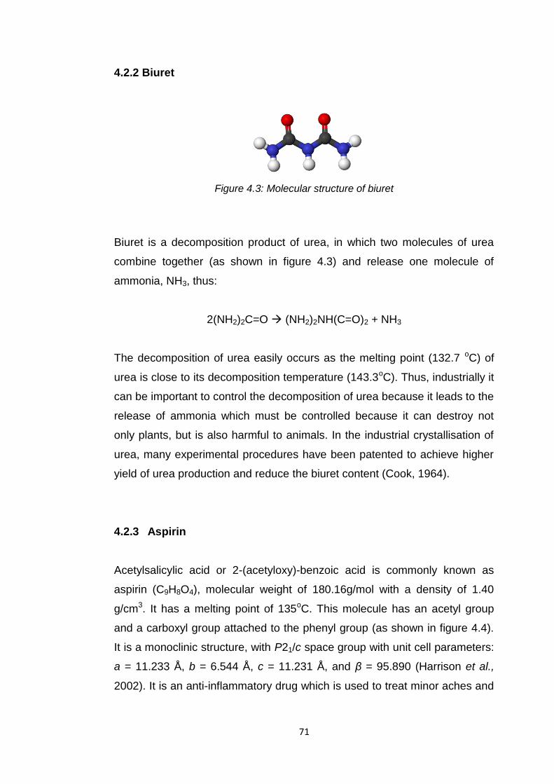
71

4.2.2 Biuret

Figure 4.3: Molecular structure of biuret

Biuret is a decomposition product of urea, in which two molecules of urea

combine together (as shown in figure 4.3) and release one molecule of

ammonia, NH3, thus:

2(NH2)2C=O (NH2)2NH(C=O)2 + NH3

The decomposition of urea easily occurs as the melting point (132.7 oC) of

urea is close to its decomposition temperature (143.3oC). Thus, industrially it

can be important to control the decomposition of urea because it leads to the

release of ammonia which must be controlled because it can destroy not

only plants, but is also harmful to animals. In the industrial crystallisation of

urea, many experimental procedures have been patented to achieve higher

yield of urea production and reduce the biuret content (Cook, 1964).

4.2.3 Aspirin

Acetylsalicylic acid or 2-(acetyloxy)-benzoic acid is commonly known as

aspirin (C9H8O4), molecular weight of 180.16g/mol with a density of 1.40

g/cm3. It has a melting point of 135oC. This molecule has an acetyl group

and a carboxyl group attached to the phenyl group (as shown in figure 4.4).

It is a monoclinic structure, with P21/c space group with unit cell parameters:

a = 11.233 Å, b = 6.544 Å, c = 11.231 Å, and β = 95.890 (Harrison et al.,

2002). It is an anti-inflammatory drug which is used to treat minor aches and

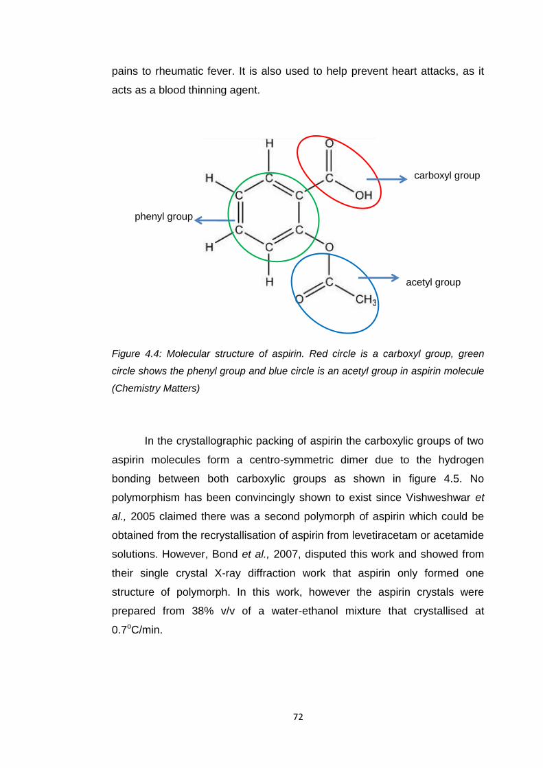
72

pains to rheumatic fever. It is also used to help prevent heart attacks, as it

acts as a blood thinning agent.

Figure 4.4: Molecular structure of aspirin. Red circle is a carboxyl group, green

circle shows the phenyl group and blue circle is an acetyl group in aspirin molecule

(Chemistry Matters)

In the crystallographic packing of aspirin the carboxylic groups of two

aspirin molecules form a centro-symmetric dimer due to the hydrogen

bonding between both carboxylic groups as shown in figure 4.5. No

polymorphism has been convincingly shown to exist since Vishweshwar et

al., 2005 claimed there was a second polymorph of aspirin which could be

obtained from the recrystallisation of aspirin from levetiracetam or acetamide

solutions. However, Bond et al., 2007, disputed this work and showed from

their single crystal X-ray diffraction work that aspirin only formed one

structure of polymorph. In this work, however the aspirin crystals were

prepared from 38% v/v of a water-ethanol mixture that crystallised at

0.7oC/min.

carboxyl group

acetyl group

phenyl group

73

Figure 4.5: The formation of the aspirin-aspirin dimer due to hydrogen bonds

between two carboxylic groups (Kim et al., 1985).

4.2.4 L-Glutamic Acid

Figure 4.6: Molecular Structure of (a) α- and (b) β-L-glutamic acid

L-glutamic acid (LGA), (C5H9NO4) has a molecular weight of 147.13g/mol

and density of 1.46 g/cm3 at 20oC. It is a non-essential amino acid. It is one

of two amino acids that have a carboxylic acid group as a side chain. It is

also known as glutamate as the carboxylic acid side chain can become

protonated, thus giving the carboxyl group a negative charge. In the human

body, this amino acids acts as neurotransmitter in which it helps nerve cells

to receive information from and to other cells. LGA has two polymorphs, the

........

........

(a) (b)

74

& β form, which are the metastable and stable form, respectively. Both

polymorphs have orthorhombic P212121 unit cells with a = 10.282, b = 8.779,

and c = 7.068 for the α-form while for the β-form, the unit cell parameters are

a = 5.159, b = 17.30, and c = 6.948 (Lehman et al., 1972), (Lehman &

Nunes, 1980). The stable β-form is needle-like in shape, while the

metastable α-form is prismatic in shape. The α form can be produced by

rapid cooling of the LGA recrystallised in aqueous solution. Heating up a

saturated solution of LGA in water with some α form crystals present in the

solution to 45˚C will transform α to β-LGA (Kitamura, 1989).

4.3 Experimental Methods

4.3.1 Crystallisation of Urea and Urea Modified by Biuret using

AutoMATE crystalliser

The crystallisation experiment of urea was carried out by AutoMATE from

HEL Ltd (as shown in figure 4.7). It is a crystalliser system consisting four

jacketed reactors equipped with stirrer, temperature detectors and turbidity

probes. All reactors can operate simultaneously with different conditions

since each reactor temperature can be controlled independently. At first, two

samples of urea were prepared and crystallised at a cooling rate of

0.1oC/min and left overnight to observe the formation of urea crystals without

and with biuret. 12g of urea was prepared in two glass flask reactors with a

capacity of 100ml while 0.5g of biuret added in one of them. 100ml ethanol

was used as a solvent to dissolve the samples. The solutions were heated

up to 60oC to ensure all the solids dissolved and then cooled down to 35oC.

Later, five sets of urea solutions were prepared with the same conditions as

the previous sets, and crystallised at five different cooling rates (0.1, 0.25,

0.5, 0.75, and 1.0oC/min). Another five sets of samples were also prepared

with the addition of biuret and five cooling rates.

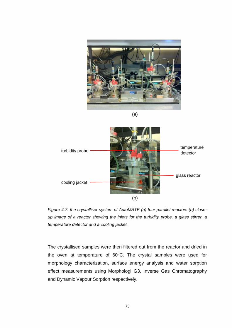
75

(a)

(b)

Figure 4.7: the crystalliser system of AutoMATE (a) four parallel reactors (b) close-

up image of a reactor showing the inlets for the turbidity probe, a glass stirrer, a

temperature detector and a cooling jacket.

The crystallised samples were then filtered out from the reactor and dried in

the oven at temperature of 60oC. The crystal samples were used for

morphology characterization, surface energy analysis and water sorption

effect measurements using Morphologi G3, Inverse Gas Chromatography

and Dynamic Vapour Sorption respectively.

turbidity probe

cooling jacket

glass reactor

temperature

detector

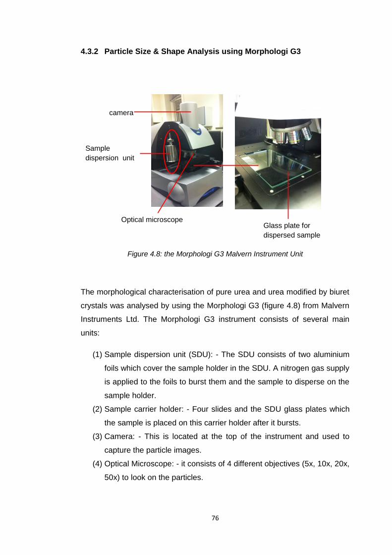
76

4.3.2 Particle Size & Shape Analysis using Morphologi G3

Figure 4.8: the Morphologi G3 Malvern Instrument Unit

The morphological characterisation of pure urea and urea modified by biuret

crystals was analysed by using the Morphologi G3 (figure 4.8) from Malvern

Instruments Ltd. The Morphologi G3 instrument consists of several main

units:

(1) Sample dispersion unit (SDU): - The SDU consists of two aluminium

foils which cover the sample holder in the SDU. A nitrogen gas supply

is applied to the foils to burst them and the sample to disperse on the

sample holder.

(2) Sample carrier holder: - Four slides and the SDU glass plates which

the sample is placed on this carrier holder after it bursts.

(3) Camera: - This is located at the top of the instrument and used to

capture the particle images.

(4) Optical Microscope: - it consists of 4 different objectives (5x, 10x, 20x,

50x) to look on the particles.

Optical microscope

Sample

dispersion unit

Glass plate for

dispersed sample

camera

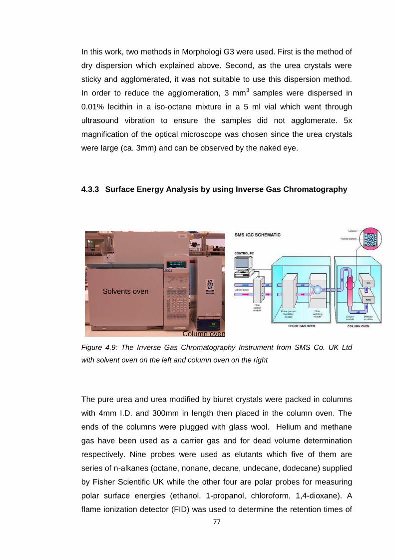
77

In this work, two methods in Morphologi G3 were used. First is the method of

dry dispersion which explained above. Second, as the urea crystals were

sticky and agglomerated, it was not suitable to use this dispersion method.

In order to reduce the agglomeration, 3 mm3 samples were dispersed in

0.01% lecithin in a iso-octane mixture in a 5 ml vial which went through

ultrasound vibration to ensure the samples did not agglomerate. 5x

magnification of the optical microscope was chosen since the urea crystals

were large (ca. 3mm) and can be observed by the naked eye.

4.3.3 Surface Energy Analysis by using Inverse Gas Chromatography

Figure 4.9: The Inverse Gas Chromatography Instrument from SMS Co. UK Ltd

with solvent oven on the left and column oven on the right

The pure urea and urea modified by biuret crystals were packed in columns

with 4mm I.D. and 300mm in length then placed in the column oven. The

ends of the columns were plugged with glass wool. Helium and methane

gas have been used as a carrier gas and for dead volume determination

respectively. Nine probes were used as elutants which five of them are

series of n-alkanes (octane, nonane, decane, undecane, dodecane) supplied

by Fisher Scientific UK while the other four are polar probes for measuring

polar surface energies (ethanol, 1-propanol, chloroform, 1,4-dioxane). A

flame ionization detector (FID) was used to determine the retention times of

Column oven

Solvents oven

78

elutants and methane. The Dorris-Gray and Schultz approaches were used

to determine surface energy determination. The surface energy calculations

were calculated using SMS-iGC Analysis Macros (version 1.8). All the

theories of calculations have been described in chapter 3. All the

experiments were undertaken at 35oC and 0% relative humidity.

4.3.4 Water Sorption Isotherm Measurement using Dynamic Vapour

Sorption

Figure 4.10: Dynamic Vapour Soprtion Unit from Surface Measurement System Co.

UK Ltd.

The quantification of water sorption effect to the surface layer of urea

samples was measured by Dynamic Vapour Sorption (figure 4.10) using

equipment obtained from Surface Measurement System Co. UK Ltd. The

samples were weighed onto a sample cup in the range of 15-10 mg using

Cahn D-200 ultra-sensitive recording microbalance. The microbalance was

placed in a fully temperature controlled incubator with ± 0.1oC temperature

stability. Because it is very sensitive to sorption and desorption of moisture,

and to avoid condensation of vapour occurring on the balance, a constant

flow rate of dry gas was supplied to purge the balance head to ensure the

baseline stability of the balance. A carrier gas, nitrogen, was used to

Sample

balance

Solvent/water

container

Analysis

software

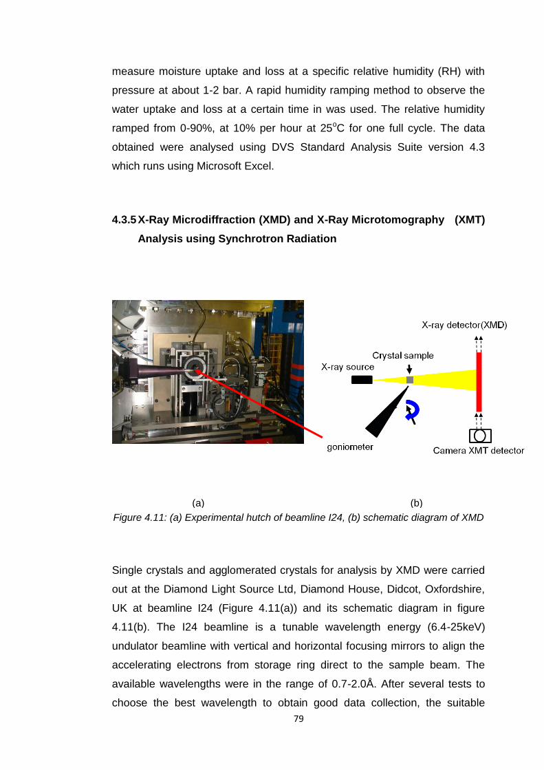
79

measure moisture uptake and loss at a specific relative humidity (RH) with

pressure at about 1-2 bar. A rapid humidity ramping method to observe the

water uptake and loss at a certain time in was used. The relative humidity

ramped from 0-90%, at 10% per hour at 25oC for one full cycle. The data

obtained were analysed using DVS Standard Analysis Suite version 4.3

which runs using Microsoft Excel.

4.3.5 X-Ray Microdiffraction (XMD) and X-Ray Microtomography (XMT)

Analysis using Synchrotron Radiation

Figure 4.11: (a) Experimental hutch of beamline I24, (b) schematic diagram of XMD

Single crystals and agglomerated crystals for analysis by XMD were carried

out at the Diamond Light Source Ltd, Diamond House, Didcot, Oxfordshire,

UK at beamline I24 (Figure 4.11(a)) and its schematic diagram in figure

4.11(b). The I24 beamline is a tunable wavelength energy (6.4-25keV)

undulator beamline with vertical and horizontal focusing mirrors to align the

accelerating electrons from storage ring direct to the sample beam. The

available wavelengths were in the range of 0.7-2.0Å. After several tests to

choose the best wavelength to obtain good data collection, the suitable

(a) (b)

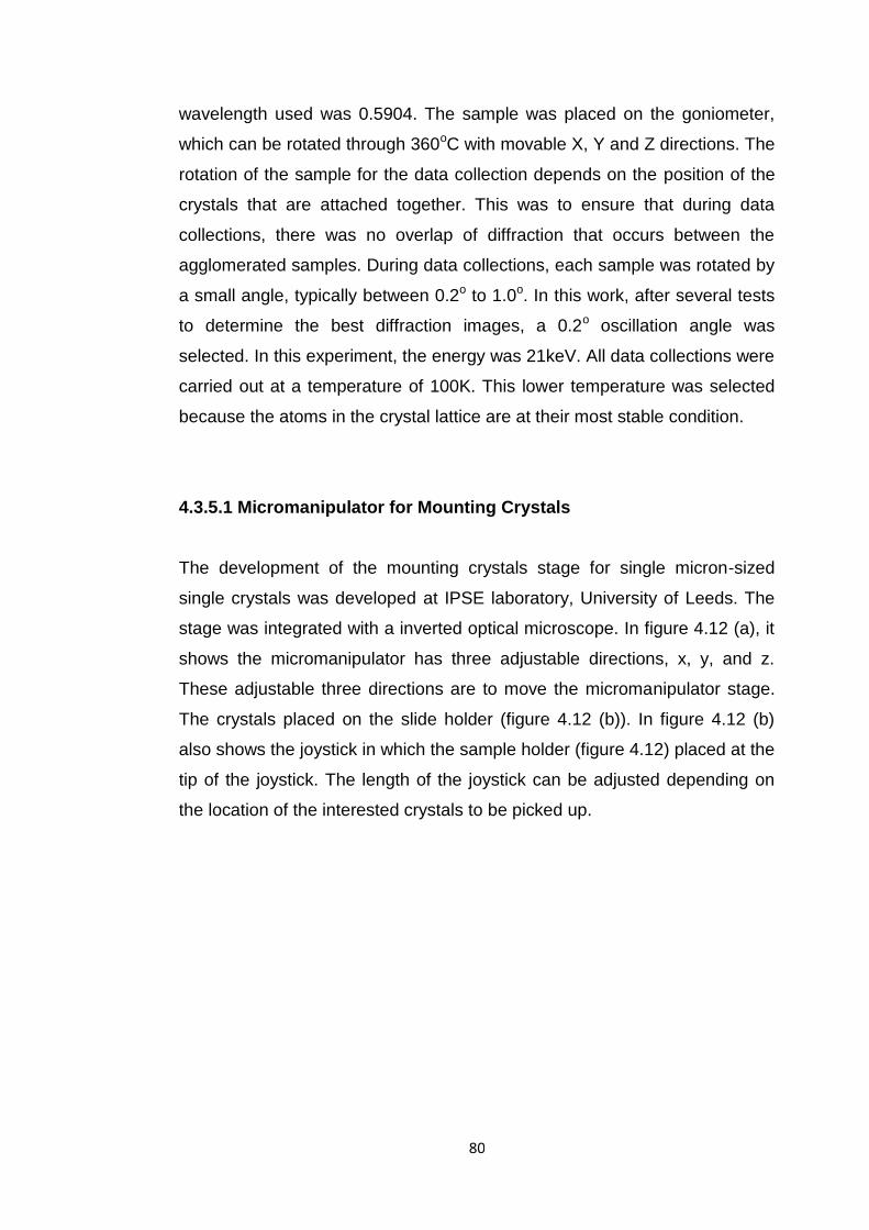
80

wavelength used was 0.5904. The sample was placed on the goniometer,

which can be rotated through 360oC with movable X, Y and Z directions. The

rotation of the sample for the data collection depends on the position of the

crystals that are attached together. This was to ensure that during data

collections, there was no overlap of diffraction that occurs between the

agglomerated samples. During data collections, each sample was rotated by

a small angle, typically between 0.2o to 1.0o. In this work, after several tests

to determine the best diffraction images, a 0.2o oscillation angle was

selected. In this experiment, the energy was 21keV. All data collections were

carried out at a temperature of 100K. This lower temperature was selected

because the atoms in the crystal lattice are at their most stable condition.

4.3.5.1 Micromanipulator for Mounting Crystals

The development of the mounting crystals stage for single micron-sized

single crystals was developed at IPSE laboratory, University of Leeds. The

stage was integrated with a inverted optical microscope. In figure 4.12 (a), it

shows the micromanipulator has three adjustable directions, x, y, and z.

These adjustable three directions are to move the micromanipulator stage.

The crystals placed on the slide holder (figure 4.12 (b)). In figure 4.12 (b)

also shows the joystick in which the sample holder (figure 4.12) placed at the

tip of the joystick. The length of the joystick can be adjusted depending on

the location of the interested crystals to be picked up.

81

(a)

(b)

Figure 4.12: The stage developed for micromanipulator for mounting single crystals.

(a) shows three adjustable directions for micromanipulator (b) adjustable joystick to

pick up the selected crystals.

4.3.5.2 Sample preparation

Single and agglomerated crystals were picked under a microscope using a

spine standard sample holder (with HamptonTM pin) with a goniometer mount

(the magnet holds the sample holder on the goniometer) (figure 4.13). After

the selection of crystals, the sample holder was mounted onto the

goniometer head. To make sure the sample was placed at the centre of the

micromanipulator stage

stage built next to

the microscope

stage can be moved x, y, and z directions

X

z

y

the length of

joystick can be

adjusted

slide holder

82

X-ray beam, the goniometer was adjusted x, y and z directions. This was

adjusted remotely by the computerised program.

Figure 4.13: Sample holder for mounting crystal

4.3.5.3 Diffraction data Collection and Processing

The diffraction data were recorded on a Pilatus3 6M, (100Hz max. frame

rate), a hybrid pixel detector from Dectris. The wavelength used in this work

was 0.5904 Å with detector distance of 220mm. There are several software

can be used to process the diffraction data for indexing and integrating to

determine the space group and the unit cell parameters. In this work, as the

samples were small molecules, the suitable softwares are X-ray Detector

Software (XDS) (Kabsch, 2001) and Xprep (Bruker, 2004) for integrating and

indexing of the diffraction data obtained from the crystal. The data obtained

was refined using Shelx (Sheldrick, 2008), a process delivering the structure

solution and refinement.

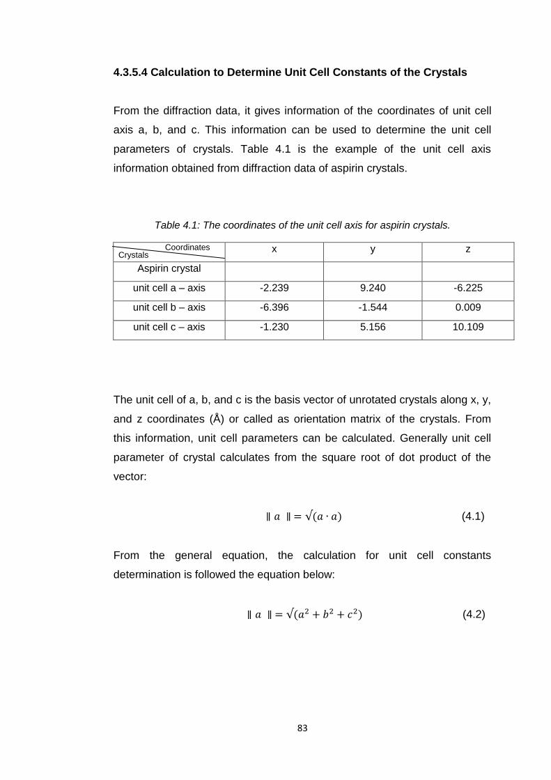
83

4.3.5.4 Calculation to Determine Unit Cell Constants of the Crystals

From the diffraction data, it gives information of the coordinates of unit cell

axis a, b, and c. This information can be used to determine the unit cell

parameters of crystals. Table 4.1 is the example of the unit cell axis

information obtained from diffraction data of aspirin crystals.

Table 4.1: The coordinates of the unit cell axis for aspirin crystals.

x y z

Aspirin crystal

unit cell a – axis -2.239 9.240 -6.225

unit cell b – axis -6.396 -1.544 0.009

unit cell c – axis -1.230 5.156 10.109

The unit cell of a, b, and c is the basis vector of unrotated crystals along x, y,

and z coordinates (Å) or called as orientation matrix of the crystals. From

this information, unit cell parameters can be calculated. Generally unit cell

parameter of crystal calculates from the square root of dot product of the

vector:

(4.1)

From the general equation, the calculation for unit cell constants

determination is followed the equation below:

(4.2)

Crystals Coordinates

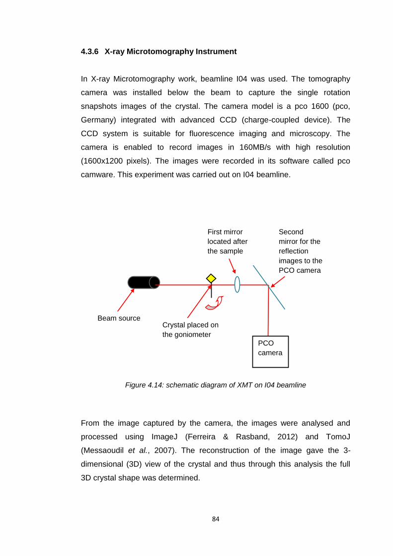
84

4.3.6 X-ray Microtomography Instrument

In X-ray Microtomography work, beamline I04 was used. The tomography

camera was installed below the beam to capture the single rotation

snapshots images of the crystal. The camera model is a pco 1600 (pco,

Germany) integrated with advanced CCD (charge-coupled device). The

CCD system is suitable for fluorescence imaging and microscopy. The

camera is enabled to record images in 160MB/s with high resolution

(1600x1200 pixels). The images were recorded in its software called pco

camware. This experiment was carried out on I04 beamline.

Figure 4.14: schematic diagram of XMT on I04 beamline

From the image captured by the camera, the images were analysed and

processed using ImageJ (Ferreira & Rasband, 2012) and TomoJ

(Messaoudil et al., 2007). The reconstruction of the image gave the 3-

dimensional (3D) view of the crystal and thus through this analysis the full

3D crystal shape was determined.

PCO

camera

Beam source Crystal placed on

the goniometer

First mirror

located after

the sample

Second

mirror for the

reflection

images to the

PCO camera

85

4.4 Computational Modelling Methods

4.4.1 Calculation of Intermolecular Interaction Using HABIT98 and

Visual Habit

The HABIT98 (Clydesdale, et al., 1998) were used to calculate the strength

of intermolecular interactions and these were, in turn, used to predict the

morphology of the urea crystals. Using this program, it calculates the

energies of solid state crystallised particles. This program predicts the

morphology of the crystal by using the Crystallographic Information File (CIF

file) that can be obtained from Cambridge Structure Database (CSD). Based

on this information, the program does not only consider the symmetry

operations of the crystal, but it also calculates the energies between

molecules based on the atomic charges calculated from quantum chemistry

calculations. In HABIT98, bonded and non-bonded forces in molecules are

used to calculate the energies of the structure. This program considers all

inter-atomic interactions between molecules both within the unit cell and the

extended lattice. These van der Waals interactions between each pair of

non-bonded atoms involved both repulsion and attraction interactions and

were calculated using either Lennard-Jones(Oobatake & Ooi, 1972) and

Buckingham potentials (Buckingham, 1938). The electrostatic energy, also

involving both repulsion and attraction interactions, was also taken into

account to give a summation of the total atom-atom energy. The total

interaction energy is calculated by defining the limiting radius of a sphere. In

this study, the limiting radius was chosen to be 30Å. The summation of all

the interaction energies is the lattice energy of the crystal (Elatt) which

consists of the slice energy (Esl) and attachment energy (Eatt). The

interaction of molecules that are close enough to the origin molecule

considered to be inside a growth layer, or slice, of thickness dhkl, in which hkl

is the growth face, and attachment energy for molecules outside of this slice.

Elatt = Esl + Eatt (4.3)

86

Figure 4.15: Limiting radius determination for lattice energy calculation

In HABIT98, the lattice energy can be calculated by choosing the

lattice (LATT) mode, while to get information of the bonding analysis of

atom-atom interactions, the FULL mode was chosen. However, for the urea

crystals, because it is a polar molecule, to obtain attachment energy of each

face of the crystal, the polar (POLR) mode was chosen. Details of HABIT98

program is in a manual by Clydesdale et al., 1998. In prediction of the urea

crystals, Lifson and Hagler force-field was used to calculate the lattice and

attachment energies. Because of the polarity of the molecule, two charges

have been used in order to calculate the attachment energy of the faces,

which were bulk charges and isolated charges that the charges of incoming

molecule to the growth layer. The charges obtained from Docherty, 1989,

calculated again using Lifson & Hagler potential set and scaled charges for

the isolated charges.

Lattice planes

(hkl)

dhkl/2

Limiting radius for

summation

dhkl

87

Visual Habit is the newer version of the HABIT98 program and one in

the process of being integrated within the CCDC’s materials Mercury

module. It has been design to be more users friendly as it has an integrated

ability to do visualisations of the crystal morphology. As in HABIT98, it

calculates the attachment energy, which uses SHAPE program to visualise

the morphology prediction based on the attachment energy values.

However, there is a limitation for this software in that it currently only has few

force-fields available to calculate the lattice energy, which Hagler force-field

is not available for the calculation. Thus, in prediction of morphology of urea

and urea modified by biuret, both morphologies were predicted by giving the

input files with values of centre to face distance for each faces.

4.4.2 Charges Calculation

In this study, three types of determining urea charges were used to

calculate the lattice energy of urea, and determine the most highest

dispersive interactions contributed in the energy, in which in later calculation

would be used for dispersive surface energy prediction. All the charges

produced from MOPAC for three different Hamiltonian parameters (AM1,

MNDO, and PM3), ab-initio quantum charges from CRYSTAL, and Hagler

scaled charges.

4.4.3 Surface Energy Prediction

In surface energy prediction calculation, the surface energy, γ for each form

(hkl) is calculated using equation 4.4. The attachment energy value obtained

from HABIT98 calculation (Hammond, et al., 2006).

88

(4.4)

Where is the surface energy of (hkl) face, (kcal/m2),

is the attachment energy of the (hkl) face, (kcal/mol),

is the interplanar spacing of (hkl) plane, (Å),

is the number of molecule in unit cell,

is the Avogadro number, and

is the cell volume of the crystal, m3

The total surface energy for the crystal was predicted from:

(4.5)

Where M is the multiplicity of the same form of the (hkl) faces and SA is the

fractional surface area of the (hkl) face. The value of multiplicity, M, together

with fractional surface area, SA, was calculated using Visual Habit. In order

to determine respectively dispersive component of the surface energies and

electrostatic energy of the crystal, the calculated values for the attachment

energy were partitioned into their van der Waals (dispersive) and

electrostatic (polar) components.

4.5 Closing Remarks

In this chapter, the materials and instruments used in this study were

discussed. The description of materials which are urea, biuret, and aspirin

were described. The methods used in preparation of the samples and the

surface analytical techniques and development of X-ray diffraction and

tomography methods also were described in detail. Additionally, the

computational methods for morphology prediction using HABIT98 and Visual

Habit and was described in this chapter.

89

References

32. Bond, A.D., Boese, R., Desiraju, G.R., (2007). On the Polymorphism

of Aspirin. Angew. Chem. Int. Ed. (46) 615-617.

33. Bruker (2004). APEX2, SAINT-Plus, XPREP and SADABS. Bruker

AXS Inc., Madison, Wisconsin, USA.

34. Buckingham, R.A,.(1938). The Classical Equation of State of

Gaseous Helium, Neon, and Argon. Proc. R. Soc. Lond. A: Math.,

Phys. Eng. Sci. (168) 264-283.

35. Clydesdale, G., Hammond, R.B., Roberts, K.J., Docherty, R., (1998).

HABIT98 - A Program for Predicting the Morphology of Molecular

Crystals as a Function of the Growth Environment. Program Manual.

36. Cook, L.H., (1964). Urea Crystallisation. United States Patent Office.

3124612.

37. Davey, R., Fila, W., Garside, J., (1986). The Influence of Biuret on the

Growth Kinetics of Urea Crystals from Aqueous Solution. J. Cryst.

Growth. (79) 607-613.

38. Docherty, R. (1989). Modelling the Morphology of Molecular Crystals.

Ph.D Thesis, University of Strathclyde, Glasgow.

39. Docherty, R., Roberts, K.J., Saunders, V., Black, S., Davey, R.J.,

(1993). Theoretical Analysis of the Polar Morphology and Absolute

Polarity of Crystalline Urea. Faraday Discuss. (95) 11-25.

40. Ferrari, E.S., Davey, R. J., (2004). Solution-Mediated Transformation

of α-to β-L-glutamic acid: Rate Enhancement Due to Secondary

Nucleation. J. Cryst. Growth Des. (4) 1061 – 1068.

41. Ferreira, T., Rasband, W., (2012). ImageJ User Guide (Revised

Edition).

42. Geddes, A., (2003). The Filtration and Drying Behaviour of Organic

Crystals with Varied Morphologies following their Batch

Crystallisation. PhD Thesis, University of Leeds.

43. Hammond, R.B., Pencheva, K., Roberts, K.J., (2006). A Structural-

Kinetic Approach to Model Face-Specific Solution/Crystal Surface

Energy Associated with the Crystallisation of Acetyl Salicylic Acid

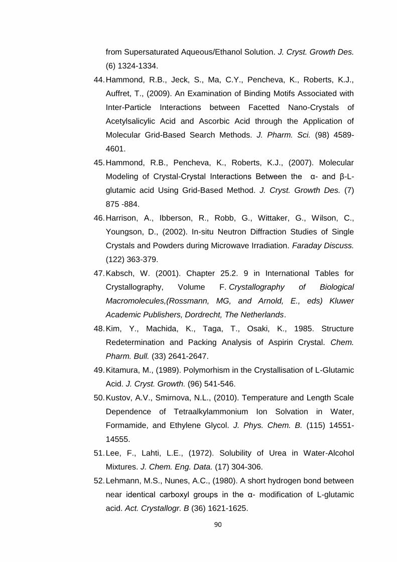
90

from Supersaturated Aqueous/Ethanol Solution. J. Cryst. Growth Des.

(6) 1324-1334.

44. Hammond, R.B., Jeck, S., Ma, C.Y., Pencheva, K., Roberts, K.J.,

Auffret, T., (2009). An Examination of Binding Motifs Associated with

Inter-Particle Interactions between Facetted Nano-Crystals of

Acetylsalicylic Acid and Ascorbic Acid through the Application of

Molecular Grid-Based Search Methods. J. Pharm. Sci. (98) 4589-

4601.

45. Hammond, R.B., Pencheva, K., Roberts, K.J., (2007). Molecular

Modeling of Crystal-Crystal Interactions Between the α- and β-L-

glutamic acid Using Grid-Based Method. J. Cryst. Growth Des. (7)

875 -884.

46. Harrison, A., Ibberson, R., Robb, G., Wittaker, G., Wilson, C.,

Youngson, D., (2002). In-situ Neutron Diffraction Studies of Single

Crystals and Powders during Microwave Irradiation. Faraday Discuss.

(122) 363-379.

47. Kabsch, W. (2001). Chapter 25.2. 9 in International Tables for

Crystallography, Volume F. Crystallography of Biological

Macromolecules,(Rossmann, MG, and Arnold, E., eds) Kluwer

Academic Publishers, Dordrecht, The Netherlands.

48. Kim, Y., Machida, K., Taga, T., Osaki, K., 1985. Structure

Redetermination and Packing Analysis of Aspirin Crystal. Chem.

Pharm. Bull. (33) 2641-2647.

49. Kitamura, M., (1989). Polymorhism in the Crystallisation of L-Glutamic

Acid. J. Cryst. Growth. (96) 541-546.

50. Kustov, A.V., Smirnova, N.L., (2010). Temperature and Length Scale

Dependence of Tetraalkylammonium Ion Solvation in Water,

Formamide, and Ethylene Glycol. J. Phys. Chem. B. (115) 14551-

14555.

51. Lee, F., Lahti, L.E., (1972). Solubility of Urea in Water-Alcohol

Mixtures. J. Chem. Eng. Data. (17) 304-306.

52. Lehmann, M.S., Nunes, A.C., (1980). A short hydrogen bond between

near identical carboxyl groups in the α- modification of L-glutamic

acid. Act. Crystallogr. B (36) 1621-1625.

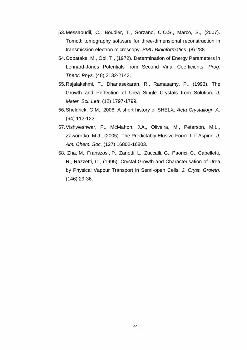
91

53. Messaoudil, C., Boudier, T., Sorzano, C.O.S., Marco, S., (2007).

TomoJ: tomography software for three-dimensional reconstruction in

transmission electron microscopy. BMC Bioinformatics. (8) 288.

54. Oobatake, M., Ooi, T., (1972). Determination of Energy Parameters in

Lennard-Jones Potentials from Second Virial Coefficients. Prog.

Theor. Phys. (48) 2132-2143.

55. Rajalakshmi, T., Dhanasekaran, R., Ramasamy, P., (1993). The

Growth and Perfection of Urea Single Crystals from Solution. J.

Mater. Sci. Lett. (12) 1797-1799.

56. Sheldrick, G.M., 2008. A short history of SHELX. Acta Crystallogr. A.

(64) 112-122.

57. Vishweshwar, P., McMahon, J.A., Oliveira, M., Peterson, M.L.,

Zaworotko, M.J., (2005). The Predictably Elusive Form II of Aspirin. J.

Am. Chem. Soc. (127) 16802-16803.

58. Zha, M., Franszosi, P., Zanotti, L., Zuccalli, G., Paorici, C., Capelletti,

R., Razzetti, C., (1995). Crystal Growth and Characterisation of Urea

by Physical Vapour Transport in Semi-open Cells. J. Cryst. Growth.

(146) 29-36.

92

CHAPTER V

INFLUENCE OF CRYSTALLISATION ENVIRONMENT ON

SURFACE PROPERTIES OF UREA

93

5.1 Introduction

This chapter discusses the results obtained from the crystallisation

experiments for urea and the effect of biuret on the formation of the urea

crystals. The aim is to understand how the addition of biuret molecules

changes the urea morphology, and also how the solution cooling rate effect

the size of particles. The analysis of the resultant size and shape using

Morphologi G3 will be presented and discussed. The effect of morphology

on surface energy of the urea and how this change for urea modified by the

presence of biuret also will be presented, together with the characterisation

of these materials propensity for water sorption using Dynamic Vapour

Sorption (DVS). To understand and rationalise the experimental results, the

molecular modelling work is used to predict crystal morphology and

molecule to surface binding of solvents and biuret interactions were used.

The work is integrated at the particle level through quantitative calculations

of surface energy of each of the crystal faces present in crystal morphology.

5.2 Experimental Studies

5.2.1 Morphological Habit Measurement Using Morphologi G3

Urea has been chosen to be studied as it has unique characteristic, as it is a

polar molecule, with different polarity at different ends. Crystalisation of urea

itself in ethanol solvent without any additive expected to produce long

needle-like crystal. However, the addition of biuret expected to change its

morphology, hence, it is an interest to understand the effect of biuret on the

morphology of urea, hence its surface properties, in this study is the surface

energy and the potential of the crystals in the water adsorption. Here, in this

experimental work, the differences of morphological habits as in size and

shape of the crystals among all the samples sets were characterised using

the Morphologi G3 instrument. The morphology differences between two

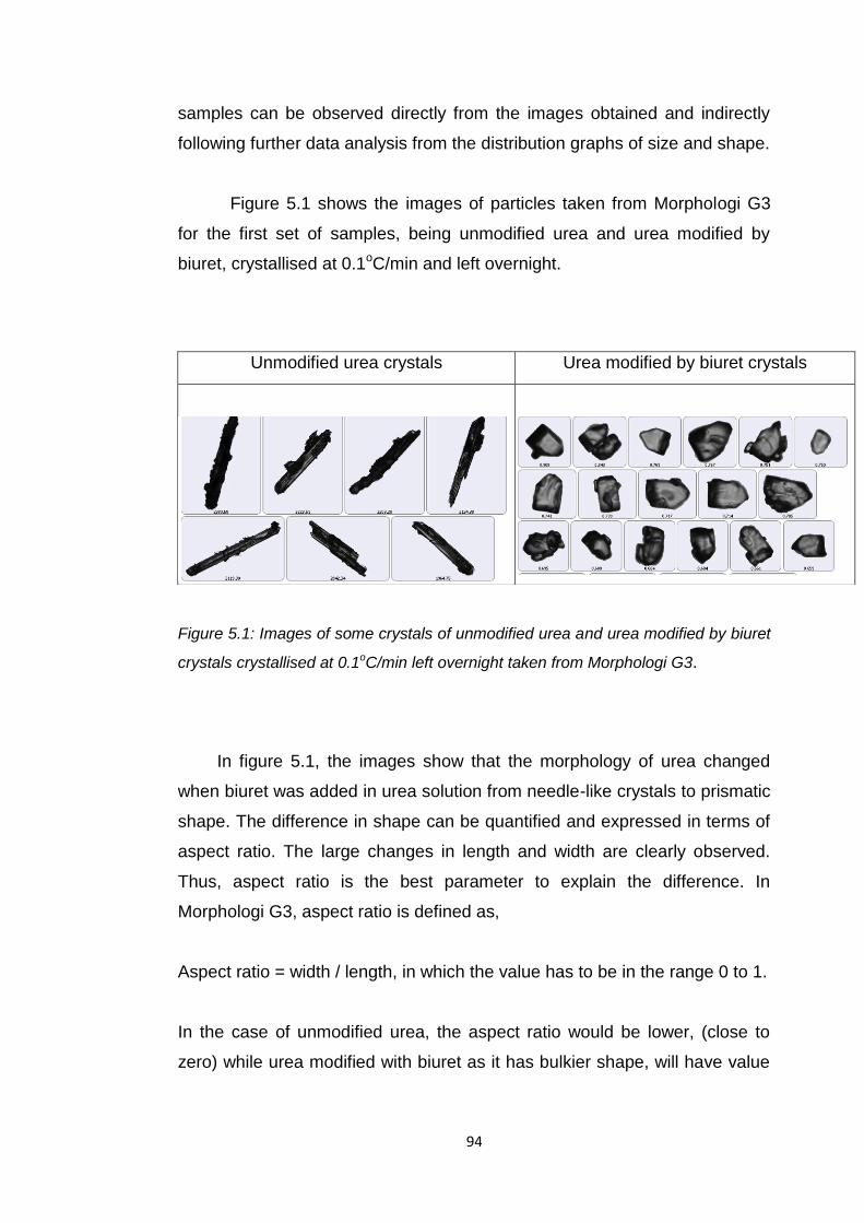
94

samples can be observed directly from the images obtained and indirectly

following further data analysis from the distribution graphs of size and shape.

Figure 5.1 shows the images of particles taken from Morphologi G3

for the first set of samples, being unmodified urea and urea modified by

biuret, crystallised at 0.1oC/min and left overnight.

Figure 5.1: Images of some crystals of unmodified urea and urea modified by biuret

crystals crystallised at 0.1oC/min left overnight taken from Morphologi G3.

In figure 5.1, the images show that the morphology of urea changed

when biuret was added in urea solution from needle-like crystals to prismatic

shape. The difference in shape can be quantified and expressed in terms of

aspect ratio. The large changes in length and width are clearly observed.

Thus, aspect ratio is the best parameter to explain the difference. In

Morphologi G3, aspect ratio is defined as,

Aspect ratio = width / length, in which the value has to be in the range 0 to 1.

In the case of unmodified urea, the aspect ratio would be lower, (close to

zero) while urea modified with biuret as it has bulkier shape, will have value

Unmodified urea crystals Urea modified by biuret crystals

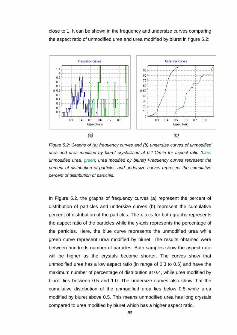
95

close to 1. It can be shown in the frequency and undersize curves comparing

the aspect ratio of unmodified urea and urea modified by biuret in figure 5.2:

(a) (b)

Figure 5.2: Graphs of (a) frequency curves and (b) undersize curves of unmodified

urea and urea modified by biuret crystallised at 0.1˚C/min for aspect ratio (blue:

unmodified urea, green: urea modified by biuret) Frequency curves represent the

percent of distribution of particles and undersize curves represent the cumulative

percent of distribution of particles.

In Figure 5.2, the graphs of frequency curves (a) represent the percent of

distribution of particles and undersize curves (b) represent the cumulative

percent of distribution of the particles. The x-axis for both graphs represents

the aspect ratio of the particles while the y-axis represents the percentage of

the particles. Here, the blue curve represents the unmodified urea while

green curve represent urea modified by biuret. The results obtained were

between hundreds number of particles. Both samples show the aspect ratio

will be higher as the crystals become shorter. The curves show that

unmodified urea has a low aspect ratio (in range of 0.3 to 0.5) and have the

maximum number of percentage of distribution at 0.4, while urea modified by

biuret lies between 0.5 and 1.0. The undersize curves also show that the

cumulative distribution of the unmodified urea lies below 0.5 while urea

modified by biuret above 0.5. This means unmodified urea has long crystals

compared to urea modified by biuret which has a higher aspect ratio.

96

Later, the crystals were crystallised at different cooling rates to observe the

effect of cooling rates on the crystals’ formation. Figure 5.3 shows the data

as a function of solution cooling rate associated with crystallisation at five

different cooling rates (0.1 0.25, 0.5, 0.75, and 1.0oC/min).

Figure 5.3: Crystal images of some of particles on samples of unmodified urea and

urea modified at different cooling rate (the number displayed on the each single

images is CE diameter number which just used for selection of single particle image

Cooling rates

(oC/min)

Unmodified urea

Urea modified by biuret

0.1

0.25

0.5

0.75

1.0

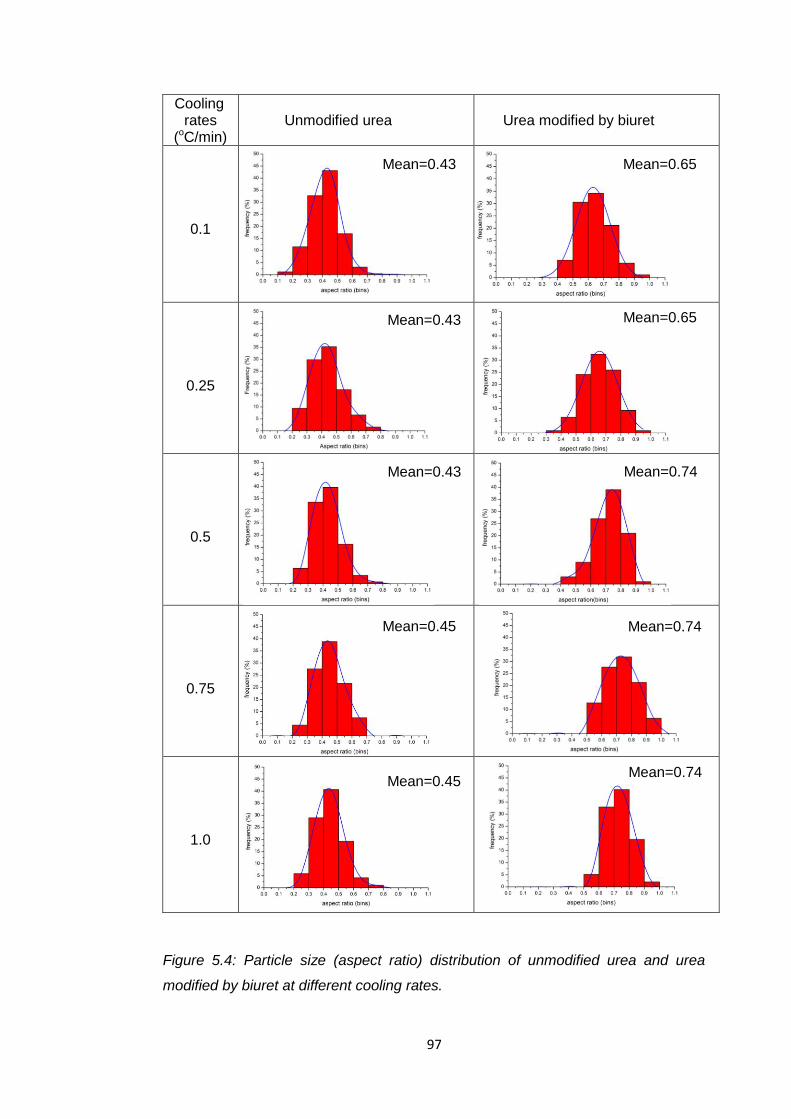
97

Figure 5.4: Particle size (aspect ratio) distribution of unmodified urea and urea

modified by biuret at different cooling rates.

Cooling rates

(oC/min)

Unmodified urea

Urea modified by biuret

0.1

0.25

0.5

0.75

1.0

Mean=0.43

Mean=0.65 Mean=0.43

Mean=0.65 Mean=0.43

Mean=0.74

Mean=0.45

Mean=0.74

Mean=0.45 Mean=0.74

Mean=0.74

Mean=0.74

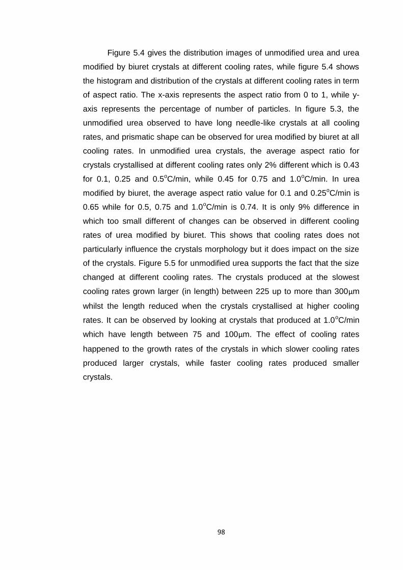
98

Figure 5.4 gives the distribution images of unmodified urea and urea

modified by biuret crystals at different cooling rates, while figure 5.4 shows

the histogram and distribution of the crystals at different cooling rates in term

of aspect ratio. The x-axis represents the aspect ratio from 0 to 1, while y-

axis represents the percentage of number of particles. In figure 5.3, the

unmodified urea observed to have long needle-like crystals at all cooling

rates, and prismatic shape can be observed for urea modified by biuret at all

cooling rates. In unmodified urea crystals, the average aspect ratio for

crystals crystallised at different cooling rates only 2% different which is 0.43

for 0.1, 0.25 and 0.5oC/min, while 0.45 for 0.75 and 1.0oC/min. In urea

modified by biuret, the average aspect ratio value for 0.1 and 0.25oC/min is

0.65 while for 0.5, 0.75 and 1.0oC/min is 0.74. It is only 9% difference in

which too small different of changes can be observed in different cooling

rates of urea modified by biuret. This shows that cooling rates does not

particularly influence the crystals morphology but it does impact on the size

of the crystals. Figure 5.5 for unmodified urea supports the fact that the size

changed at different cooling rates. The crystals produced at the slowest

cooling rates grown larger (in length) between 225 up to more than 300μm

whilst the length reduced when the crystals crystallised at higher cooling

rates. It can be observed by looking at crystals that produced at 1.0oC/min

which have length between 75 and 100μm. The effect of cooling rates

happened to the growth rates of the crystals in which slower cooling rates

produced larger crystals, while faster cooling rates produced smaller

crystals.

99

Figure 5.5: Distribution graph of unmodified urea at different cooling rate indicates

that the length of the crystals decreasing at the faster cooling rates.

5.2.2 Surface Energy Analysis Study Using Inverse Gas

Chromatography

The study of surface energies of urea and urea modified by biuret has been

carried out using IGC using several organic solvents as probes in order to

determine the dispersive surface energies of the samples. In the first case,

sets of samples of unmodified urea and urea modified by biuret at 0.1oC/min

which were left in the reactors overnight to undergo uncontrolled

crystallisation were prepared. Each sample was measured three times to

obtain reproducible results. The surface energy results obtained are

tabulated in table 5.1:

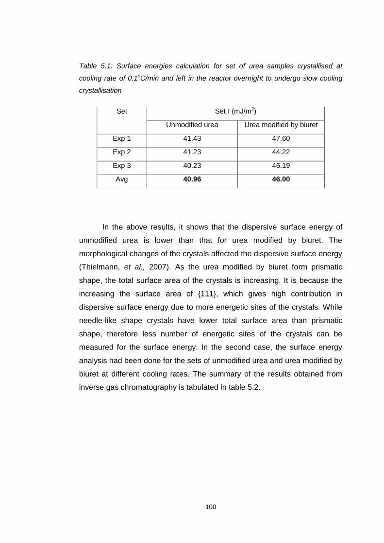
100

Table 5.1: Surface energies calculation for set of urea samples crystallised at

cooling rate of 0.1oC/min and left in the reactor overnight to undergo slow cooling

crystallisation

In the above results, it shows that the dispersive surface energy of

unmodified urea is lower than that for urea modified by biuret. The

morphological changes of the crystals affected the dispersive surface energy

(Thielmann, et al., 2007). As the urea modified by biuret form prismatic

shape, the total surface area of the crystals is increasing. It is because the

increasing the surface area of {111}, which gives high contribution in

dispersive surface energy due to more energetic sites of the crystals. While

needle-like shape crystals have lower total surface area than prismatic

shape, therefore less number of energetic sites of the crystals can be

measured for the surface energy. In the second case, the surface energy

analysis had been done for the sets of unmodified urea and urea modified by

biuret at different cooling rates. The summary of the results obtained from

inverse gas chromatography is tabulated in table 5.2.

Set Set I (mJ/m2)

Unmodified urea Urea modified by biuret

Exp 1 41.43 47.60

Exp 2 41.23 44.22

Exp 3 40.23 46.19

Avg 40.96 46.00

101

Table 5.2: Summary of dispersive surface energy results for unmodified urea and

urea modified by biuret at different cooling rates

Figure 5.6: Dispersive surface energy plotted of unmodified urea and urea modified

by biuret at different cooling rates.

The data presented in Table 5.2 and plotted as a graph in Figure 5.6,

shows that increasing cooling rate for crystallisation to occur, the surface

energy becomes higher. The same trend of increasing in surface energy can

be observed for unmodified urea and urea modified by biuret samples. As

Samples Unmodified urea Urea modified by biuret

Cooling

rates

(°C/min)

0.1

0.25

0.5

0.75

1.0

0.1

0.25

0.5

0.75

1.0

Run 1 39.51 42.2 43.57 44.33 45.62 43.00 43.2 45.85 46.69 47.11

Run 2 40.79 42.18 43.78 44.47 45.32 42.28 43.72 45.07 46.67 47.35

Run 3 41.80 42.99 44.19 44.19 45.52 42.15 43.31 45.28 46.6 46.35

Avg

Surface

energy

(mJ/m2)

40.7

42.5

43.9

44.3

45.5

42.5

43.4

45.4

46.7

46.9

y = 4.8692x + 40.832

R² = 0.9297

y = 5.2363x + 42.252

R² = 0.9407

40

42

44

46

48

0 0.5 1

dis

pers

ive s

urf

ace e

nerg

y

(mJ/m

2)

cooling rate (°C/min)

Dispersive surface energy vs cooling rates

urea crystals

urea with biuret

Linear (urea crystals)

Linear (urea with biuret)

102

increasing the cooling rates to allow the crystallisation to occur, the crystals

produced were smaller. This is because the time for the crystals to grow

completely is too fast at the higher cooling rates, in consequence, small

crystals were produced and give impact to the surface area of the crystals.

In contrast, at slower cooling rates, for example crystals crystallised at

cooling rate of 0.1oC/min, the crystals produced were larger. Therefore,

changes in cooling rates affect the value of dispersive surface energy

because of increasing in surface are per volume of the crystals.

5.2.3 Dynamic Vapour Sorption Studies

Data from the water sorption experiments and analysis using DVS to

observe the effect of water taken in unmodified urea and urea modified by

biuret samples is shown in Figure 5.7. These reveal the percentage of mass

changes of unmodified urea and urea modified by biuret crystals at different

cooling rates. The mass changes of the samples were observed at different

relative humidity. Results from 0 to 70% relative humidity are showed in

figure 5.7 and figure 5.8. Cut off at 70% relative humidity had been chosen

because of at higher relative humidity than 70%, the water soprtion on the

samples are high and rapidly increase (up to 40% water uptake), which

showing that the absorption of water in samples had taken part .Graphs in

figure 5.7 are shown to discuss the effect of crystals crystallised at different

cooling rates on the rates of adsorption. Figure 5.8 shows the comparison

curves of unmodified urea and urea modified by biuret at 0.1 and 1.0oC/min

to compare the rates of adsoprtion between unmodified urea and urea

modified by biuret crystals.

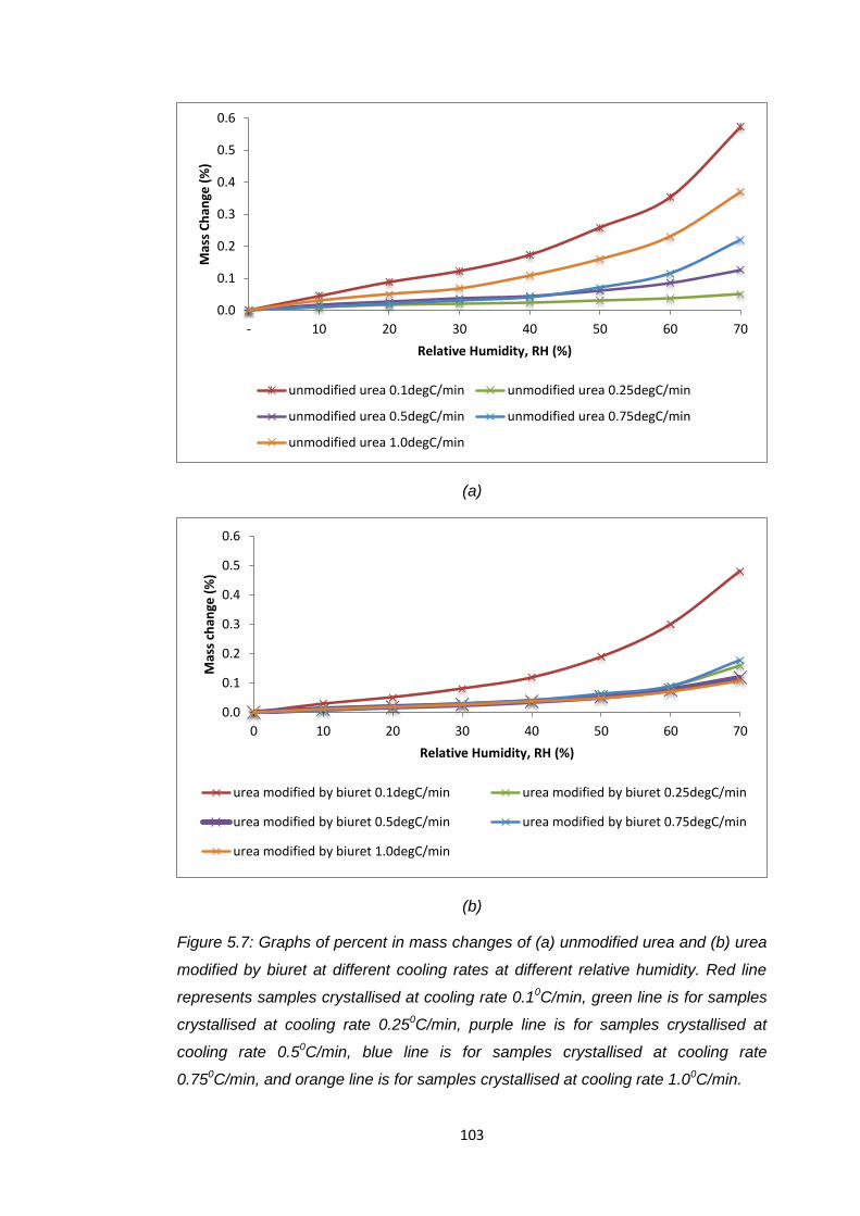
103

(a)

(b)

Figure 5.7: Graphs of percent in mass changes of (a) unmodified urea and (b) urea

modified by biuret at different cooling rates at different relative humidity. Red line

represents samples crystallised at cooling rate 0.10C/min, green line is for samples

crystallised at cooling rate 0.250C/min, purple line is for samples crystallised at

cooling rate 0.50C/min, blue line is for samples crystallised at cooling rate

0.750C/min, and orange line is for samples crystallised at cooling rate 1.00C/min.

0.0

0.1

0.2

0.3

0.4

0.5

0.6

- 10 20 30 40 50 60 70

Mas

s C

han

ge (

%)

Relative Humidity, RH (%)

unmodified urea 0.1degC/min unmodified urea 0.25degC/min

unmodified urea 0.5degC/min unmodified urea 0.75degC/min

unmodified urea 1.0degC/min

0.0

0.1

0.2

0.3

0.4

0.5

0.6

0 10 20 30 40 50 60 70

Mas

s ch

ange

(%

)


urea modified by biuret 0.1degC/min urea modified by biuret 0.25degC/min

urea modified by biuret 0.5degC/min urea modified by biuret 0.75degC/min

urea modified by biuret 1.0degC/min

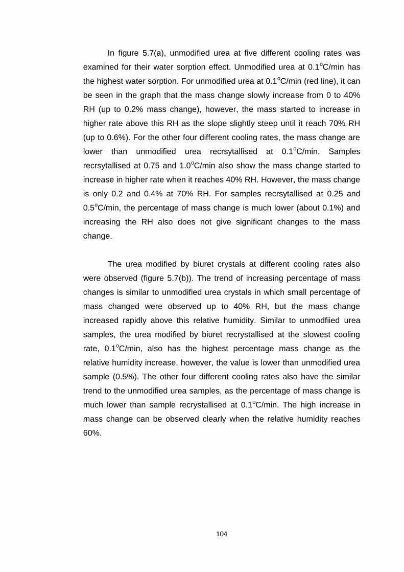
104

In figure 5.7(a), unmodified urea at five different cooling rates was

examined for their water sorption effect. Unmodified urea at 0.1oC/min has

the highest water sorption. For unmodified urea at 0.1oC/min (red line), it can

be seen in the graph that the mass change slowly increase from 0 to 40%

RH (up to 0.2% mass change), however, the mass started to increase in

higher rate above this RH as the slope slightly steep until it reach 70% RH

(up to 0.6%). For the other four different cooling rates, the mass change are

lower than unmodified urea recrsytallised at 0.1oC/min. Samples

recrsytallised at 0.75 and 1.0oC/min also show the mass change started to

increase in higher rate when it reaches 40% RH. However, the mass change

is only 0.2 and 0.4% at 70% RH. For samples recrsytallised at 0.25 and

0.5oC/min, the percentage of mass change is much lower (about 0.1%) and

increasing the RH also does not give significant changes to the mass

change.

The urea modified by biuret crystals at different cooling rates also

were observed (figure 5.7(b)). The trend of increasing percentage of mass

changes is similar to unmodified urea crystals in which small percentage of

mass changed were observed up to 40% RH, but the mass change

increased rapidly above this relative humidity. Similar to unmodfiied urea

samples, the urea modified by biuret recrystallised at the slowest cooling

rate, 0.1oC/min, also has the highest percentage mass change as the

relative humidity increase, however, the value is lower than unmodified urea

sample (0.5%). The other four different cooling rates also have the similar

trend to the unmodified urea samples, as the percentage of mass change is

much lower than sample recrystallised at 0.1oC/min. The high increase in

mass change can be observed clearly when the relative humidity reaches

60%.

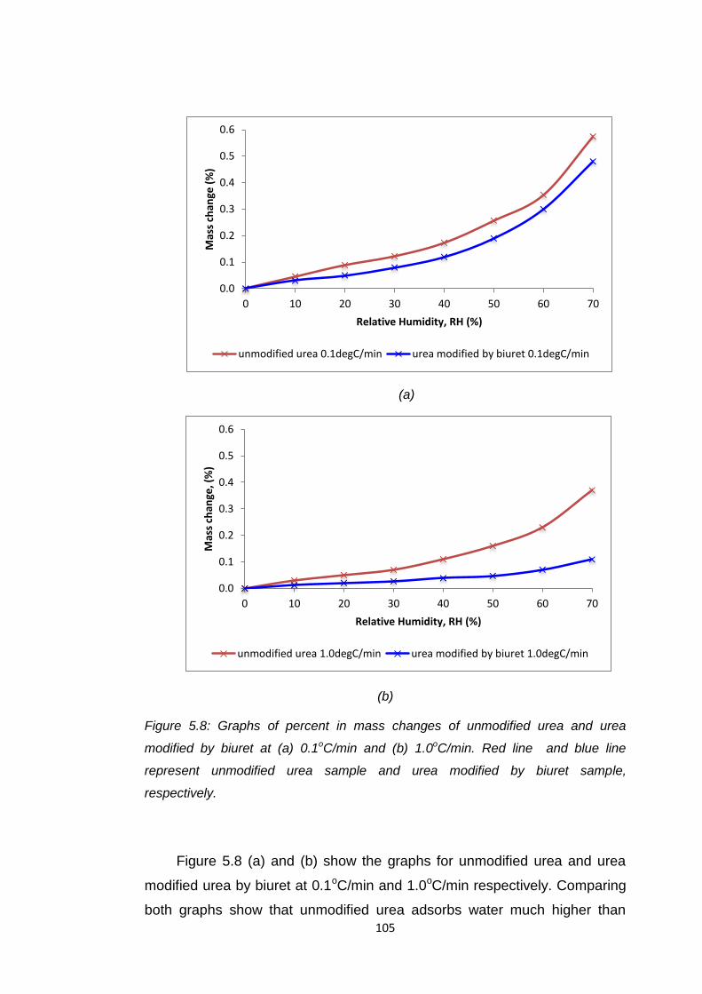
105

(a)

(b)

Figure 5.8: Graphs of percent in mass changes of unmodified urea and urea

modified by biuret at (a) 0.1oC/min and (b) 1.0oC/min. Red line and blue line

represent unmodified urea sample and urea modified by biuret sample,

respectively.

Figure 5.8 (a) and (b) show the graphs for unmodified urea and urea

modified urea by biuret at 0.1oC/min and 1.0oC/min respectively. Comparing

both graphs show that unmodified urea adsorbs water much higher than

0.0

0.1

0.2

0.3

0.4

0.5

0.6

0 10 20 30 40 50 60 70

Mas

s ch

ange

(%

)


unmodified urea 0.1degC/min urea modified by biuret 0.1degC/min

0.0

0.1

0.2

0.3

0.4

0.5

0.6

0 10 20 30 40 50 60 70

Mas

s ch

ange

, (%

)


unmodified urea 1.0degC/min urea modified by biuret 1.0degC/min

106

urea modified by biuret. It can be seen from graph that up to 70% RH, the

perecentage of mass change is 0.6 and 0.5, resplectively, eventhough only

0.1% difference. For unmodified urea at 0.1oC/min At 1.0oC/min (figure

5.7(b)), it also shows unmodified urea increased its mass higher than urea

modified by biuret. The difference is larger than samples recrystallised at

0.1oC/min., which is about 0.3% difference. Urea is expected to have very

hygroscopic characteristic (Werner, 1937). Its {110} face is known to have

hydrophilic characteristics. As unmodified urea has large surface area of

{110}, therefore has ability to adsorb water molecules from its surrounding

very easily, and hold the water molecules strongly, also, further increase in

relative humidity makes the crystals absorbed water rather than only

adsoprtion process. However, as the crystals become more prismatic, the

{110} face is shrinking, while the {111} face which less hydrophilic grew

larger. Hence, less water adsorbed at the whole surfaces of the crystals.

5.2.4 Integration of the Experimental Analysis

Crystallisation of urea in ethanol solvent produced long needle-like crystals.

This result is consistent with reports that urea crystals grow rapidly on [001]

direction, thus identifying the (001) face as the fastest growing face (Davey,

et al., 1986) crystallised in water and (Huang, et al., 1990) crystallised urea

in different solvents.

In figure 5.1, the size of unmodified urea and urea modified biuret at

0.1°C/min cooling rates showed the size became smaller. The size of

unmodified urea is long needle-like shape. However, addition of biuret to the

urea solution for crystallisation, it can be seen that the crystal become

shorter and produce smaller block shaped crystals. The difference between

size distributions of the two samples can be observed from the frequency

and undersize curves of aspect ratio of the crystals in Figure 5.2. The crystal

size of urea crystallised at 0.1°C/min were long up to 2.6 mm while the urea

modified by biuret at 0.1°C/min has average crystal size length of 100 μm.

The addition of biuret on the crystal habit affecting the relative growth rates

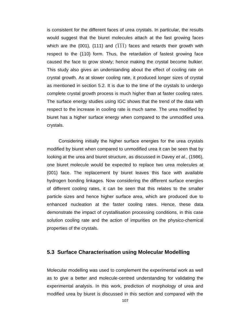
107

is consistent for the different faces of urea crystals. In particular, the results

would suggest that the biuret molecules attach at the fast growing faces

which are the {001}, {111} and faces and retards their growth with

respect to the {110} form. Thus, the retardation of fastest growing face

caused the face to grow slowly; hence making the crystal become bulkier.

This study also gives an understanding about the effect of cooling rate on

crystal growth. As at slower cooling rate, it produced longer sizes of crystal

as mentioned in section 5.2. It is due to the time of the crystals to undergo

complete crystal growth process is much higher than at faster cooling rates.

The surface energy studies using IGC shows that the trend of the data with

respect to the increase in cooling rate is much same. The urea modified by

biuret has a higher surface energy when compared to the unmodified urea

crystals.

Considering initially the higher surface energies for the urea crystals

modified by biuret when compared to unmodified urea it can be seen that by

looking at the urea and biuret structure, as discussed in Davey et al., (1986),

one biuret molecule would be expected to replace two urea molecules at

{001} face. The replacement by biuret leaves this face with available

hydrogen bonding linkages. Now considering the different surface energies

of different cooling rates, it can be seen that this relates to the smaller

particle sizes and hence higher surface area, which are produced due to

enhanced nucleation at the faster cooling rates. Hence, these data

demonstrate the impact of crystallisation processing conditions, in this case

solution cooling rate and the action of impurities on the physico-chemical

properties of the crystals.

5.3 Surface Characterisation using Molecular Modelling

Molecular modelling was used to complement the experimental work as well

as to give a better and molecule-centred understanding for validating the

experimental analysis. In this work, prediction of morphology of urea and

modified urea by biuret is discussed in this section and compared with the

108

experimental results. In addition, prediction of surface energy also calculated

using attachment energy approach.

5.3.1 Morphology Prediction of Urea

In routine work of morphology prediction of urea, attachment energy of each

crystal faces was calculated. As urea has a polar morphology with different

ends of (111) being polar, BFDH and classical attachment energy methods

cannot be directly used because BFDH method predicts the morphology

only based on the crystal geometry while the second approach does not

consider polar faces and will give the same value of attachment energy for

the polar faces (Docherty, 1989). Thus, the polar attachment energy

calculation method developed by Docherty (1989) was used to predict the

morphology of urea. In this work, the attachment energy calculation by

Docherty was initially reproduced as a reference point for these studies. In

latter calculations, the force field chosen was by Lifson and Hagler (Lifson et

al., 1979) which has good description for amides. Also, this force field has its

own charges distribution that suitable to use for urea compound. In

Docherty’s work, for self-consistency, he scaled the charges provided by

Lifson and Hagler. There were two types of charges that had been

considered for the polar morphology calculation which were the bulk isolated

charges and surface isolated charges. Bulk isolated charges are charges

that distributed by the molecule in the bulk crystal while surface isolated

charges are the charges from incoming molecule to the surface of the bulk

crystal.

5.3.1.1 Identification of Key Intermolecular Interactions

In order to predict crystal morphology, the intermolecular interactions of the

crystals need to be understand. The intermolecular interactions determine

the vaiue of the attachment energy of the crystals faces. Figure 5.9 shows

the strongest intermolecular interactions exist in urea crystal. From bonding

109

analysis calculation in HABIT98, it shows that two hydrogen bonding exists

in urea crystal (type a and b). Table 5.3 shows the intermolecular bonding

analysis in urea crystal. Figure 5.9(c) shows one molecule of urea forms

hydrogen bonds with molecules surrounding it. By taking one molecule of

urea as a central molecule (noted in yellow colour), the oxygen atom from

the central molecule can form four hydrogen bonds with the hydrogen atoms

from the surrounding molecules, while the hydrogen atoms from amides

form hydrogen bond with the oxygen atom from the molecules surround it.

Table 5.3: Debug analysis of intermolecular bonds in urea using Hagler force field

with Hagler charges.

Bond

type

multiplicity Distance

(Å)

van der Waals van der

Waals

(total)

COU

Total ATT REP

a 4 4.68 -2.02 2.10 0.08 -3.74 -3.66

b 8 4.3 -1.74 1.26 -0.48 -2.52 -3.00

110

(a) bond type a (b) bond type b

(c)

Figure 5.9: Atom-atom interaction (a) bond type a (b) bond type b from DM-analysis

(c) the hydrogen bonding interaction between central molecule of urea (yellow) with

its surrounding molecules.

5.3.1.2 Attachment Energy Calculation for Morphology Prediction

As urea is a polar molecule, the attachment energy calculation needs also to

consider the slice energy of each face. Consideration of the growth slice

position and energy for the faces is important in order to obtain the most

a

a a

a b

b

b

b

111

stable value for each of the unique habit faces. Here, four faces were taken

into account in order to predict the morphology, which is (001) as the fastest

growing face, (110) as the slowest growing face, (111) and as polar

faces. The slice energies that need to be considered are for the polar faces.

Thus, the calculations of the slice energy must reach the most stable energy,

and then the value of attachment energy is selected. From the calculations

of the slice energy as a function of its position, the value of the attachment

energy of -4.6 and -4.9 kcal/mol for {111} and {-1-1-1} respectively

calculated to give the most stable slice energy values for both faces as

plotted in graphs Figure 5.10.

Table 5.4: Summary of slice energy and attachment energy using bulk-isolated

charges

slice shift

Eslice (kcal/mol) Eatt (kcal/mol)

(1 1 1) (-1 -1 -1) (1 1 1) (-1 -1 -1)

0 -6.57 -6.57 -6.8 -6.8

0.1 -6.57 -6.57 -6.8 -6.8

0.2 -9.09 -9.09 -5.4 -5.9

0.3 -10.55 -10.55 -4.9 -5.4

0.4 -10.94 -10.94 -4.7 -5

0.5 -11.13 -11.13 -4.6 -4.9

0.6 -11.13 -11.13 -4.6 -4.9

0.7 -11.13 -11.13 -4.6 -4.9

0.8 -11.16 -11.16 -4.6 -4.9

0.9 -11.16 -11.16 -4.6 -4.9

1 -11.16 -11.16 -4.6

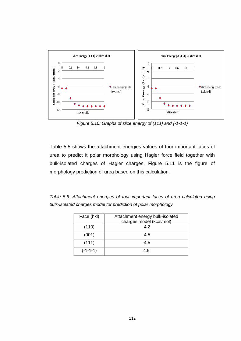
112

Figure 5.10: Graphs of slice energy of {111} and {-1-1-1}

Table 5.5 shows the attachment energies values of four important faces of

urea to predict it polar morphology using Hagler force field together with

bulk-isolated charges of Hagler charges. Figure 5.11 is the figure of

morphology prediction of urea based on this calculation.

Table 5.5: Attachment energies of four important faces of urea calculated using

bulk-isolated charges model for prediction of polar morphology

Face (hkl) Attachment energy bulk-isolated charges model (kcal/mol)

(110) -4.2

(001) -4.5

(111) -4.5

(-1-1-1) 4.9

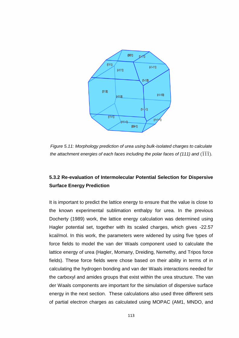
113

Figure 5.11: Morphology prediction of urea using bulk-isolated charges to calculate

the attachment energies of each faces including the polar faces of (111) and .

5.3.2 Re-evaluation of Intermolecular Potential Selection for Dispersive

Surface Energy Prediction

It is important to predict the lattice energy to ensure that the value is close to

the known experimental sublimation enthalpy for urea. In the previous

Docherty (1989) work, the lattice energy calculation was determined using

Hagler potential set, together with its scaled charges, which gives -22.57

kcal/mol. In this work, the parameters were widened by using five types of

force fields to model the van der Waals component used to calculate the

lattice energy of urea (Hagler, Momany, Dreiding, Nemethy, and Tripos force

fields). These force fields were chose based on their ability in terms of in

calculating the hydrogen bonding and van der Waals interactions needed for

the carboxyl and amides groups that exist within the urea structure. The van

der Waals components are important for the simulation of dispersive surface

energy in the next section. These calculations also used three different sets

of partial electron charges as calculated using MOPAC (AM1, MNDO, and

114

PM3 implementations), CRYSTAL and those taken from Hagler (Docherty,

1989) as well as the case without the charges on the molecule being

considered. The description of each types of charges used in lattice energy

calculations and lists of charges for all types of atoms are listed in table 5.6

and 5.7 respectively.

Table 5.6: Description of types of atoms use in lattice energy calculations for three

Hamiltonian parameters of MOPAC charges (AM1, MNDO, PM3), ab-anitio charges

from CRYSTAL, and Hagler scaled charges from its own partial charges.

Types of charges

Descriptions

AM1 Austin Model 1. Use for C, H, N, O. It is suitable for many chemical functionalities. (Dewar et al., 1985)

MNDO Modified Neglect of Differential Overlap Model 2. The parameters calculate the atomic orbital ionisation, van der Waals and electrostatic interactions (Dewar & Thiel, 1977)

PM3 Parameterised Model 3. Optimise simultanouesly C, H, N, O, F, Al, Si, P, S, Cl, Br, I. Use two parameters of Gaussian functions (Stewart, 1989)

CRYSTAL Ab-initio quantum mechanicals charges calculations

HAGLER Hagler own calculated charges. Use for carboxylic and amide groups

* Full descriptions of each types of charges can be obtained from Cramer, 2002

Table 5.7: Types of charges use in lattice energy calculations. Three types of

charges; empirical charges of MOPAC with different Hamiltanion parameters (AM1,

MNDO,PM3), ab-anitio charges from CRYSTAL, and Hagler scaled charges

Atoms Types of charges

MOPAC CRYSTAL HAGLER

AM1 MNDO PM3

Carbon (C) 0.401 0.467 0.168 0.426 0.380

Oxygen (O) -0.439 -0.455 -0.480 -0.425 -0.380

Nitrogen (N) -0.450 -0.408 0.011 -0.467 -0.830

Hydrogen (H) 0.251 0.215 0.089 0.219 0.415

Hydrogen (H) 0.218 0.187 0.057 0.196 0.415

Nitrogen (N) -0.450 -0.408 0.011 -0.467 -0.83

Hydrogen (H) 0.251 0.215 0.089 0.219 0.415

Hydrogen (H) 0.218 0.187 0.057 0.196 0.415

115

Table 5.8: Types of force-fields with their type of potential in calculating lattice

energy

Force Fields Types of potential

Hagler Parameterised for H, C, N, O: carboxylic acid and amides. Use its own partial charges to calculate lattice energy

Momany General hydrogen bond potential. Parameterised for H, C, N, O: carboxylic acid and amides. Take into account the van der Waals interactions

Dreiding Van der Waals interactions in combination of 2 and 3 body in term of hydrogen bond

Nemethy General hydrogen bond potential. Parameterised for H, C, N, O: carboxylic acid and amides.

Tripos Scaling factors for hydrogen bond. Parameterised for H, C, N, O, Cl, F, S. H-bond acceptor atoms: N, O, F, Cl, S

116

Table 5.9: Lattice energies values of urea using four different charges and five different force fields. The bold columns in black is the values using

Hagler potential with its scaled charges providing a good match to the experimental lattice energy of -22.2kcal/mol, however, provides an

unrealistically low van der Waals component. The bold columns in red is the values using Dreiding potential with CRYSTAL charges, which gives

the highest value of van der Waals component.

Force

Fields

Lattice Energy (kcal/mol)

Mopac CRYSTAL HAGLER No

charges AM1 MNDO PM3

VdW Coul Total VdW Coul Total VdW Coul Total VdW Coul Total VdW Coul Total VdW

Hagler -5.8 -10.6 -16.4 -5.9 -9.1 -15.0 -5.9 -8.6 -14.5 -5.9 -8.8 -14.7 -5.9 -16.7 -22.6 -5.9

Momany -11.4 -5.3 -16.7 -11.4 -4.5 -15.9 -11.4 -4.3 -15.6 -11.4 -4.6 -16.0 -11.4 -8.3 -19.7 -11.4

Dreiding -13.1 -10.6 -23.8 -13.1 -9.1 -22.2 -13.1 -8.6 -21.7 -13.1 -8.8 -21.9 -13.1 -16.7 -29.8 -13.1

Nemethy -4.5 -10.6 -15.1 -10.8 -4.5 -15.3 -10.7 -4.3 -15.0 -10.7 -4.4 -15.1 -10.7 -8.3 -19.1 -10.7

Tripos -4.5 -10.6 -15.1 -4.5 -9.1 -13.6 -4.4 -8.6 -13.0 -4.5 -8.8 -13.3 -4.5 -16.7 -21.2 -4.5

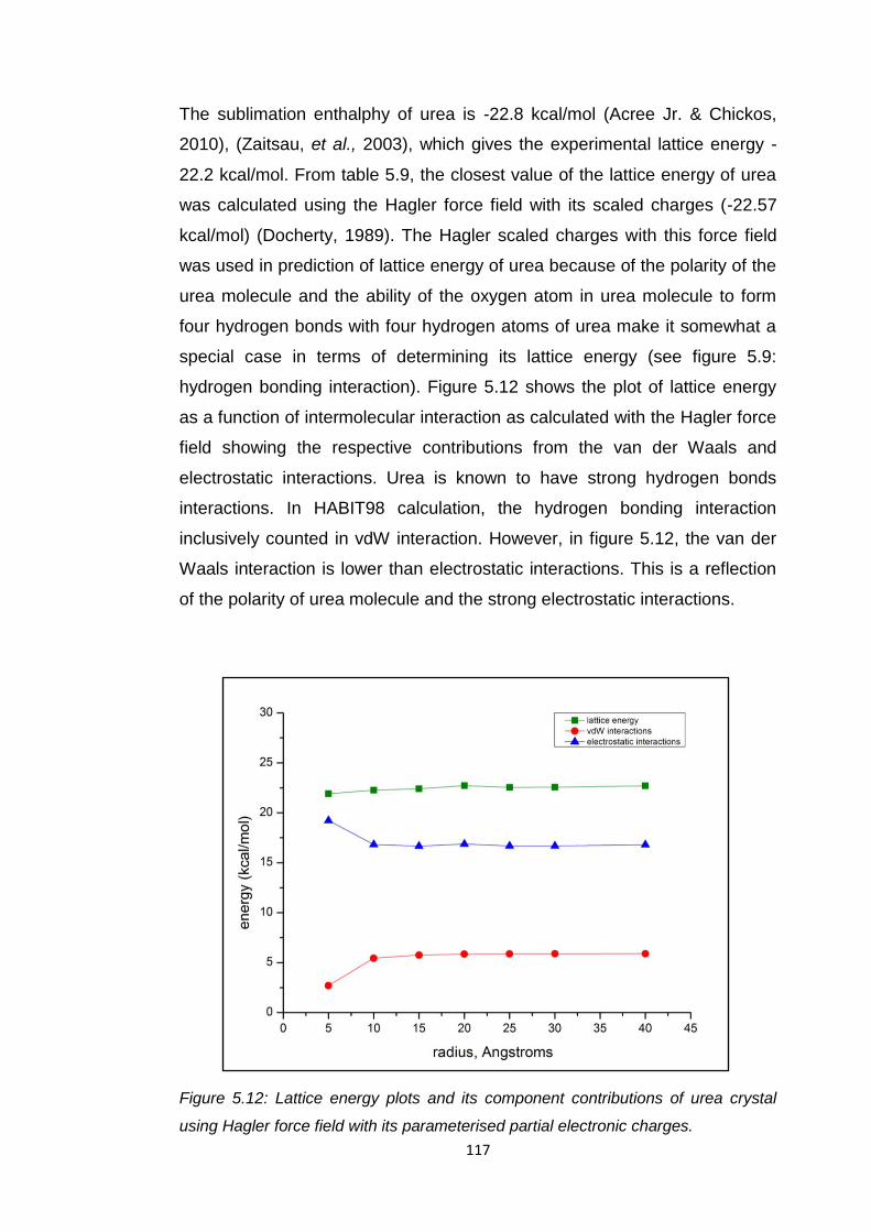
117

The sublimation enthalphy of urea is -22.8 kcal/mol (Acree Jr. & Chickos,

2010), (Zaitsau, et al., 2003), which gives the experimental lattice energy -

22.2 kcal/mol. From table 5.9, the closest value of the lattice energy of urea

was calculated using the Hagler force field with its scaled charges (-22.57

kcal/mol) (Docherty, 1989). The Hagler scaled charges with this force field

was used in prediction of lattice energy of urea because of the polarity of the

urea molecule and the ability of the oxygen atom in urea molecule to form

four hydrogen bonds with four hydrogen atoms of urea make it somewhat a

special case in terms of determining its lattice energy (see figure 5.9:

hydrogen bonding interaction). Figure 5.12 shows the plot of lattice energy

as a function of intermolecular interaction as calculated with the Hagler force

field showing the respective contributions from the van der Waals and

electrostatic interactions. Urea is known to have strong hydrogen bonds

interactions. In HABIT98 calculation, the hydrogen bonding interaction

inclusively counted in vdW interaction. However, in figure 5.12, the van der

Waals interaction is lower than electrostatic interactions. This is a reflection

of the polarity of urea molecule and the strong electrostatic interactions.

Figure 5.12: Lattice energy plots and its component contributions of urea crystal

using Hagler force field with its parameterised partial electronic charges.

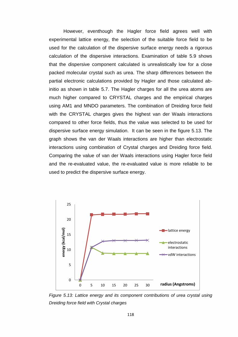
118

However, eventhough the Hagler force field agrees well with

experimental lattice energy, the selection of the suitable force field to be

used for the calculation of the dispersive surface energy needs a rigorous

calculation of the dispersive interactions. Examination of table 5.9 shows

that the dispersive component calculated is unrealistically low for a close

packed molecular crystal such as urea. The sharp differences between the

partial electronic calculations provided by Hagler and those calculated ab-

initio as shown in table 5.7. The Hagler charges for all the urea atoms are

much higher compared to CRYSTAL charges and the empirical charges

using AM1 and MNDO parameters. The combination of Dreiding force field

with the CRYSTAL charges gives the highest van der Waals interactions

compared to other force fields, thus the value was selected to be used for

dispersive surface energy simulation. It can be seen in the figure 5.13. The

graph shows the van der Waals interactions are higher than electrostatic

interactions using combination of Crystal charges and Dreiding force field.

Comparing the value of van der Waals interactions using Hagler force field

and the re-evaluated value, the re-evaluated value is more reliable to be

used to predict the dispersive surface energy.

Figure 5.13: Lattice energy and its component contributions of urea crystal using

Dreiding force field with Crystal charges

0

5

10

15

20

25

0 5 10 15 20 25 30

en

erg

y (k

cal/

mo

l)

lattice energy

electrostatic interactions

vdW interactions

radius (Angstroms)

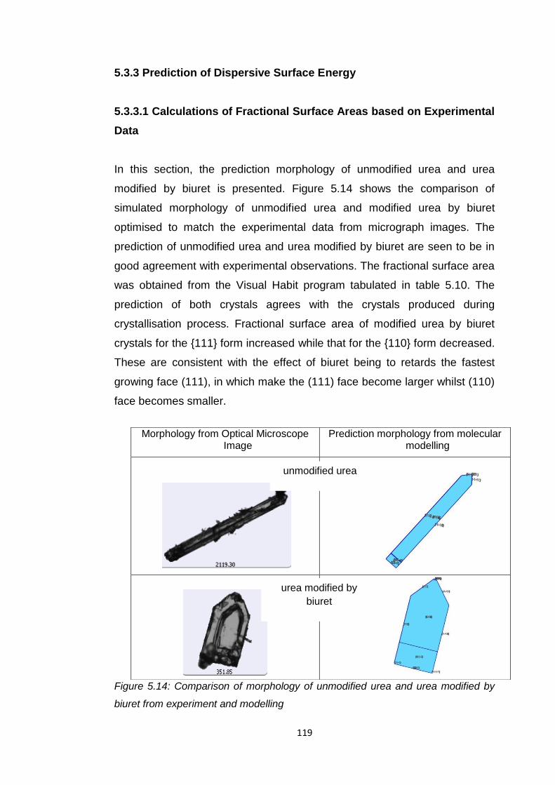
119

5.3.3 Prediction of Dispersive Surface Energy

5.3.3.1 Calculations of Fractional Surface Areas based on Experimental

Data

In this section, the prediction morphology of unmodified urea and urea

modified by biuret is presented. Figure 5.14 shows the comparison of

simulated morphology of unmodified urea and modified urea by biuret

optimised to match the experimental data from micrograph images. The

prediction of unmodified urea and urea modified by biuret are seen to be in

good agreement with experimental observations. The fractional surface area

was obtained from the Visual Habit program tabulated in table 5.10. The

prediction of both crystals agrees with the crystals produced during

crystallisation process. Fractional surface area of modified urea by biuret

crystals for the {111} form increased while that for the {110} form decreased.

These are consistent with the effect of biuret being to retards the fastest

growing face (111), in which make the (111) face become larger whilst (110)

face becomes smaller.

Figure 5.14: Comparison of morphology of unmodified urea and urea modified by

biuret from experiment and modelling

Morphology from Optical Microscope Image

Prediction morphology from molecular modelling

unmodified urea

urea modified by

biuret

120

Table 5.10: Percentage surface area of crystal faces obtained from Visual Habit

The fractional area obtained in previous section was used to calculate the

total dispersive surface energy of unmodified urea and urea modified by

biuret using surface energy prediction (equation 4.2) and its molecular scale

rationalisation. The summary of dispersive surface energy prediction is

tabulated in table 5.11. In dispersive energy prediction, the calculations were

made using all five forces. The prediction result using Dreiding force field

provided the best results for dispersive surface energy. Using dreiding force

field, the dispersive surface energy prediction gives 45.51 and 53.27 mJ/m2

for unmodified urea and urea modified urea by biuret respectively (table

5.11). The values are higher than the experimental values, which 40.96 and

46.00, respectively. However, the prediction values provided the same

trends as the experimental surface energy results, in which the modified

urea by biuret has a higher predictive dispersive surface energy when

compared to that of the unmodified urea. The stronger dispersive

interactions give by the dreiding force field are consistent with this force field

being more suitable for modelling the van der Waals interactions for a

strongly hydrogen bonded system such as urea.

Crystal Face

% Surface Area

h k l Unmodified

urea Urea Modified

by biuret

1 1 0 22.84 16.58

1 -1 0 22.84 16.58

-1 -1 0 22.84 16.58

-1 1 0 22.84 16.58

1 1 1 2.04 8.12

1 -1 -1 2.04 8.12

-1 -1 1 2.04 8.12

-1 1 -1 2.04 8.12

total 100 100

121

Table 5.11: Summary of prediction surface energy of unmodified urea and urea modified by biuret

Form

Multiplicity

(M)

Unmodified urea (mJ/m2) Urea modified by biuret

Fractional surface

area (SA)

Dispersive Surface Energy

Electrostatic Surface Energy

Total Surface Energy

Fractional surface

area (SA)

Dispersive Surface Energy

Electrostatic Surface Energy

Total Surface Energy

{1 1 0} 4 0.228 39.29

40.21

79.50 0.166

28.51

29.18

57.69

{1 1 1} 4 0.020 6.22

6.85

13.07 0.081

24.76

27.25

52.01

Total surface energy (mJ/m2) 45.51

47.06

92.57

53.27

56.43

109.70

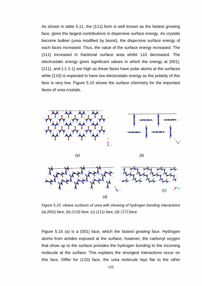
122

As shown in table 5.11, the {111} form is well known as the fastest growing

face, gives the largest contributions in dispersive surface energy. As crystals

become bulkier (urea modified by biuret), the dispersive surface energy of

each faces increased. Thus, the value of the surface energy increased. The

{111} increased in fractional surface area whilst 110 decreased. The

electrostatic energy gives significant values in which the energy at {001},

{111}, and {-1-1-1} are high as these faces have polar atoms at the surfaces

while {110} is expected to have low electrostatic energy as the polarity of this

face is very low. Figure 5.15 shows the surface chemistry for the important

faces of urea crystals.

(a) (b)

(c)

(d)

Figure 5.15: cleave surfaces of urea with showing of hydrogen bonding interactions

(a) (001) face, (b) (110) face, (c) (111) face, (d) face.

Figure 5.15 (a) is a (001) face, which the fastest growing face. Hydrogen

atoms from amides exposed at the surface, however, the carbonyl oxygen

that show up to the surface provides the hydrogen bonding to the incoming

molecule at the surface. This explains the strongest interactions occur on

this face. Differ for (110) face, the urea molecule lays flat to the other

123

molecule, therefore, the interactions to the incoming molecules are very

weak. For the polar faces, at face, the carbonyl oxygen exposed at the

surface, however, hydrogen from amides be on the (111) face.

5.4 Discussion

From all the experimental and molecular modelling analysis, the results

show that modification of crystallisation of urea by addition of biuret changed

its morphology from needle-like shape to prismatic shape. Also, the

crystallisation of both unmodified urea and urea modified by biuret at

different cooling rates gave effect to the crystals size. The change in crystal

morphology and crystal size further analysed using dynamic vapour sorption

for water sorption analysis as reveal that urea is a comparatively

hygroscopic material. Unmodified urea was found to adsorbed water to a

higher degree than urea modified by biuret. It is confirmed that crystallisation

of urea in water solution produced very needle-like shape, in which the

crystal growth at c-axis (001) is very fast. The study on dispersive surface

energy was carried out using inverse gas chromatography to understand the

effect to the dispersive surface energy. The addition of biuret increased the

dispersive surface energy while smaller crystal size gives higher dispersive

surface energy value compared to the larger crystal. The experimental work

validated using molecular modelling based upon predictions of the urea

morphology. From the attachment energy calculations and fractional surface

area determination, the prediction morphology of urea was found to agree

with the morphology observed in experimental work. The dispersive surface

energy prediction using Dreiding force field with CRYSTAL charges agrees

well with the experimental results.

124

5.5 Closing Remarks

All the experimental and molecular modelling work helps to understand the

effect of biuret to the urea crystals. The surface energy simulation analysis

give good agreement with the value obtained from experimental data. This

comparison gives understanding that the changed morphology of the actual

crystal, it also changed the overall surface properties of the crystals.

References

1. Acree, Jr, W., Chickos, J.S., (2010). J. Phys. Chem. Regf. Data Vol

39.

2. Davey, R., Fila, W., Garside, J., (1986). The Influence of Biuret on

the Growth Kinetics of Urea Crystals from Aqueous Solution. J.

Cryst. Growth. (79) 607-613.

3. Huang, B., SU, G., HE, Y., (1990). Growth of Large Size Urea

Crystals. J. Cryst. Growth. (102) 762-764.

4. Lifson, S., Hagler, A.T., Dauber, P. (1979). Consistent Force Field

Studies of Intermolecular Forces in Hydrogen-Bonded Crystals. 1.

Carboxylic Acids, Amides, and the C=OH-Hydrogen Bonds. J. Am.

Chem. Soc. (101) 5111.

5. Thielmann, F., Burnett, D.J., Heng, J.Y.Y., (2007). Determination of

the Surface Energy Distributions of Different Processed Lactose.

Drug Development and Indsutrial Pharmacy. (33):1240-1253.

6. Werner, E.A., (1937). Urea as a Hygroscopic Substance. Nature

Publishing Group. 512.

7. Zaitsau, D., Kabo, G.J., Kozyro, A.A., Sevruk, V.M., (2003).

Thermochim. Acta. (406) 17-28

125

CHAPTER VI

CHARACTERISATION OF MICRO-CRYSTALS AND THE

AGGLOMERATES USING X-RAY MICRODIFFRACTION AND

MICROTOMOGRAPHY

126

6.1 Introduction

This chapter discusses the results collected from XMD and XMT experiment

at the Diamond Light Source using the microfocus beamline I24 and the

macrocrystallography beamlike I04. There are four case studies describe in

this work. Firstly, a study the variability of crystals in powders by observing

the difference in unit cell parameters. Also, from this study, the capability of

carrying out diffraction experiment on micro-crystals of small molecules

using microfocus beamline can be explained. Three compounds were

chosen for investigation: (i) aspirin, (ii) urea and its modification by biuret (iii)

polymorphic transformation of α- to β-L-glutamic acid. Secondly an

examination aimed to understand the relationship of relative orientation

between agglomerated particles of the aspirin and urea. Angle calculation

using vector calculations and using the method of stereographic projection to

determine the angles between crystals will be discussed in this chapter.

Thirdly, is an examination of the interfacial development of the β-form

microcrystal of LGA on the surface of the α-form. Fourthly a study aimed of

understanding the external morphology of agglomerated micro-crystal and to

correlate it with the XMD result by using single XMT. This was carried out on

an agglomerated sample of α-LGA.

6.2 Justification on Selection of the Materials

As this research is focused on work on the ability of using a micro-focus

beam in order to determine the structure and orientation of the micron sized

small molecule particles, examination of other system is also important in

order to test and to produce sufficient results to prove the ability of the

overall approach itself. In this, aspirin crystals were selected as they have

smaller particles than urea, less than 50 μm, which are suitable for the

micro-focus beam used at synchrotrons. Furthermore, the aspirin crystals

like urea also formed agglomerates.

127

Urea is a polar molecule is the primary material chosen for study in

this thesis. It is a unique molecule in which one oxygen atom can form four

hydrogen bonds with hydrogen atoms surrounds it. Crystallisation of urea in

water and alcoholic solvents, such as methanol and ethanol forms long-

needle like crystals. By adding biuret to the process, the morphology

changes from long-needle shape crystals to prismatic crystals. There are

published works on the experimental study of crystallisation of urea and how

biuret affects the urea morphology (Davey, et al., 1986), and modelling work

Docherty, 1991), (Salvalaglio, et al., 2012). However, during the process

itself, the crystals often form agglomerates. Thus, it is of interest to

understand the surface chemistry properties of the urea crystals and the

difference between the urea crystals and urea modified by biuret crystals.

LGA was also chosen to be one of the systems to be studied because

it has polymorphs. The polymorphs change from metastable form of α-LGA

to stable β-LGA when the temperature increases above 45oC. Polymorphism

of LGA is also well published in which the (101) face of β-LGA crystal grew

from the (111) face of the α-LGA crystal (Ferrari & Davey, 2004),

(Hammond, et al., 2007). Thus, in this case LGA provides an opportunity to

get a better understanding on how these two polymorphs are orientated

each other during crystal growth.

6.3 Case study 1: Variability in the structure of

microcrystals within Powdered Samples

From X-ray diffraction data collection, the routine work that needs to be done

from the data collection is to process the data to determine the unit cell

parameters and the space group of the crystals. For this routine, in general,

it is not neceesary to have complete diffraction images data set from the

crystal sample. Unit cell parameters can be determined from coordinates of

unit cell a, b, and c-axis. Variation in aspirin crystals and urea and urea

modified by biuret were observed.

128

6.3.1 Variation in aspirin powder samples

Table 6.1 is the results of unit cell parameters of aspirin for each crystals

obtained from the processed data collection with the standard deviation (std.

dev.) in the bracket.

Table 6.1: Summary of unit cell constant determination for aspirin crystals

a b c β mosaicity

Crystal 1 11.251 6.530 11.237 95.87 0.301

Crystal 2 11.238 6.539 11.244 95.92 0.298

Crsytal 3 11.239 6.543 11.242 95.91 0.282

Crystal 4 11.240 6.541 11.242 95.91 0.265

Crystal 5 11.239 6.541 11.245 95.92 0.288

Crystal 6 11.240 6.541 11.242 95.92 0.276

Crystal 7 11.261 6.518 11.256 95.86 0.268

Crystal 8 11.241 6.539 11.239 95.90 0.256

Crystal 9 11.239 6.541 11.238 95.91 0.289

Crystal 10 11.239 6.547 11.242 95.92 0.279

Crystal 11 11.240 6.543 11.238 95.92 0.283

Crystal 12 11.241 6.537 11.244 95.89 0.289

Average value

(Std Dev)

11.242

(0.007)

6.539

(0.007)

11.242

(0.005)

95.90

(0.02)

0.281

(0.013)

Unit cell constants of aspirin from literature : a = 11.242, b = 6.539, c = 11.245

(Aubrey et al., 2007)

Unit cell (Ao)

(A°)

Crystals

129

In this work, the objective is to observe the variability of unit cell

constants for sample to sample within a powdered sample. For most studies

to determine the unit cell constants of single crystal, large single crystals

were used. By using synchrotron technology, it is possible to use small

single micro-crystal to measure the unit cell constants. In this study, twelve

aspirin single micro-crystals had been mounted for data collection. From the

processed data of these single crystals of aspirin, the space group was

determined to be P21/c and monoclinic with 4 molecules per unit cell, in

which agreed with other aspirin crystal structure determination (Wheatley,

1964). In the experiment that was carried out, the structure of aspirin had

been solved and compared with several literatures. Solving the aspirin

structure is to do comparison on the result of data collection using

microfocus beamline X-ray microdiffraction and conventional X-ray

diffraction (Wheatley, 1964 and Kim et al, 1984), also other diffraction

method such as neutron diffraction (Harrison, 2002). Figure 6.1 shows the

molecular structure of aspirin sample as solved using SHELX in the WinGX

program (Farrugia, 2012). The R-factor value for this solving structure is

0.05. The literature value of R-factor was 0.18 and 0.04 respectively for X-

ray diffraction and 0.09 for neutron diffraction. The unit cell constants values

were found to be very similar to each other. The average unit cell constants

for all collected data was found to be a = 11.242, b = 6.539, c = 11.242, and

β = 95.90. The values of a and c axes were found to be almost the same

and to all intents and purpose can be concluded to be identical. These

values were compared with literature (bottom column in table 6.1) with which

only a very small difference was observed. The values were determined

from single crystal XRD. The unit cell constants also compared with different

method such as neutron diffraction to determine crystal structure of aspirin

and the results were also found to agree with it (Harrison et al., 2002). The

percentage error obtained from results of the data processing show only a

very small error in the unit cell constants values. Thus this work showed that

there was no significant change in unit cell constants of crystals in a batch of

powder crystals.

130

Figure 6.1: Aspirin crystal structure visualise in CAMERON graphical tool plugged-

in WinGX software.

6.3.2 Variability in the Structure of Micro-crystals as a Function of

Processing Conditions

The second material studied using XMD was urea. In this XMD data was

collected from unmodified urea and urea modified by biuret micro-crystals

prepared at five different cooling rates. Table 6.2 to 6.11 shows the unit cell

constants for all the samples, urea and urea with addition of biuret at 0.1,

0.25, 0.5, 0.75 and 1.0 ˚C/min respectively. The unit cell parameters of urea

crystal structure from literature to be used as comparison was a = b =

5.565Å, c = 4.684Å and α, β, γ = 90˚. This material has a tetragonal structure

with a P-421m space group.

131

Table 6.2: Unit cell constants of urea 0.1oC/min

a b c mosaicity

Crystal 1 5.620 5.620 4.688 0.226

Crystal 2 5.626 5.626 4.693 0.286

Crsytal 3 5.623 5.623 4.691 0.210

Crystal 4 5.622 5.622 4.690 0.194

Crystal 5 5.564 5.564 4.679 0.148

Crystal 6 5.571 5.571 4.677 0.377

Crsytal 7 5.565 5.565 4.679 0.144

Crystal 8 5.566 5.566 4.679 0.220

Crystal 9 5.566 5.566 4.679 0.284

Crsytal 10 5.570 5.570 4.679 0.218

Crystal 11 5.577 5.577 4.683 0.197

Crystal 12 5.567 5.567 4.679 0.140

Average Unit

Cell Parameters

and std dev ( ) 5.586 (0.027) 5.586 (0.027) 4.683 (0.006)

0.220

(0.069)

Unit cell (Å) Crystals

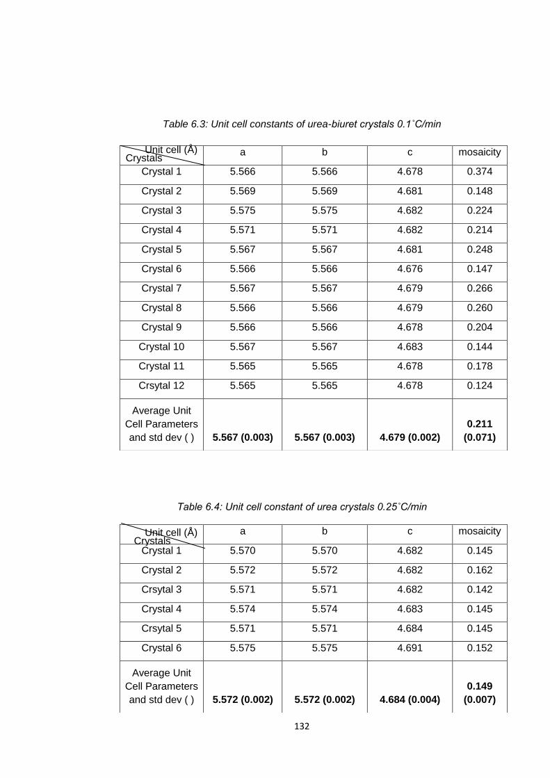
132

Table 6.3: Unit cell constants of urea-biuret crystals 0.1˚C/min

Table 6.4: Unit cell constant of urea crystals 0.25˚C/min

a b c mosaicity

Crystal 1 5.566 5.566 4.678 0.374

Crystal 2 5.569 5.569 4.681 0.148

Crystal 3 5.575 5.575 4.682 0.224

Crystal 4 5.571 5.571 4.682 0.214

Crystal 5 5.567 5.567 4.681 0.248

Crystal 6 5.566 5.566 4.676 0.147

Crystal 7 5.567 5.567 4.679 0.266

Crystal 8 5.566 5.566 4.679 0.260

Crystal 9 5.566 5.566 4.678 0.204

Crystal 10 5.567 5.567 4.683 0.144

Crystal 11 5.565 5.565 4.678 0.178

Crsytal 12 5.565 5.565 4.678 0.124

Average Unit

Cell Parameters

and std dev ( ) 5.567 (0.003) 5.567 (0.003) 4.679 (0.002)

0.211

(0.071)

a b c mosaicity

Crystal 1 5.570 5.570 4.682 0.145

Crystal 2 5.572 5.572 4.682 0.162

Crsytal 3 5.571 5.571 4.682 0.142

Crystal 4 5.574 5.574 4.683 0.145

Crsytal 5 5.571 5.571 4.684 0.145

Crystal 6 5.575 5.575 4.691 0.152

Average Unit

Cell Parameters

and std dev ( ) 5.572 (0.002) 5.572 (0.002) 4.684 (0.004)

0.149

(0.007)



133

Table 6.5: Unit cell constant of urea-biuret crystals 0.25degC/min

Table 6.6: Unit cell constants of urea crystals 0.5˚C/min

a b c mosaicity

Crystal 1 5.574 5.574 4.684 0.151

Crystal 2 5.571 5.571 4.681 0.365

Crsytal 3 5.569 5.569 4.681 0.142

Crystal 4 5.567 5.567 4.681 0.393

Crsytal 5 5.571 5.571 4.678 0.167

Crystal 6 5.569 5.569 4.681 0.146

Crystal 7 5.576 5.576 4.685 0.147

Crystal 8 5.572 5.572 4.682 0.160

Average Unit

Cell Parameters

and std dev ( ) 5.571 (0.003) 5.571 (0.003) 4.682 (0.002)

0.209

(0.106)

a b c mosaicity

Crystal 1 5.565 5.565 4.678 0.155

Crystal 2 5.566 5.566 4.678 0.143

Crsytal 3 5.563 5.563 4.677 0.166

Crystal 4 5.565 5.565 4.679 0.147

Average Unit

Cell Parameters

and std dev ( ) 5.565 (0.001) 5.565 (0.001) 4.678 (0.001)

0.152

(0.010)

Crystals

Unit cell (Å)

Crystals

Unit cell (Å)

Crystals

Crystals

Crystals

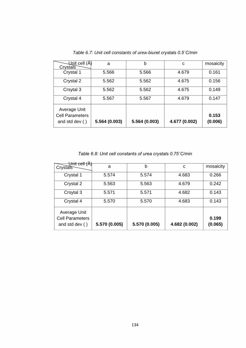
134



a b c mosaicity

Crystal 1 5.566 5.566 4.679 0.161

Crystal 2 5.562 5.562 4.675 0.156

Crsytal 3 5.562 5.562 4.675 0.149

Crystal 4 5.567 5.567 4.679 0.147

Average Unit

Cell Parameters

and std dev ( ) 5.564 (0.003) 5.564 (0.003) 4.677 (0.002)

0.153

(0.006)

a b c mosaicity

Crystal 1 5.574 5.574 4.683 0.266

Crystal 2 5.563 5.563 4.679 0.242

Crsytal 3 5.571 5.571 4.682 0.143

Crystal 4 5.570 5.570 4.683 0.143

Average Unit

Cell Parameters

and std dev ( ) 5.570 (0.005) 5.570 (0.005) 4.682 (0.002)

0.199

(0.065)



135



a b c mosaicity

Crystal 1 5.567 5.567 4.681 0.372

Crystal 2 5.572 5.572 4.682 0.246

Crsytal 3 5.566 5.566 4.680 0.412

Crystal 4 5.566 5.566 4.680 0.443

Crystal 5 5.567 5.567 4.677 0.143

Crystal 6 5.570 5.570 4.682 0.272

Crystal 7 5.562 5.562 4.676 0.262

Crystal 8 5.563 5.563 4.675 0.147

Crystal 9 5.564 5.564 4.679 0.167

Crystal 10 5.568 5.568 4.679 0.142

Crystal 11 5.568 5.568 4.679 0.163

Crsytal 12 5.567 5.567 4.679 0.160

Crystal 13 5.566 5.566 4.678 0.140

Average Unit

Cell Parameters

and std dev ( ) 5.567 (0.003) 5.567 (0.003) 4.679 (0.002)

0.236

(0.110)

a b c mosaicity

Crystal 1 5.574 5.574 4.682 0.413

Crystal 2 5.571 5.571 4.679 0.446

Crsytal 3 5.579 5.579 4.697 0.272

Crystal 4 5.569 5.569 4.694 0.333

Average Unit

Cell Parameters

and std dev ( ) 5.573 (0.004) 5.573 (0.004) 4.688 (0.009)

0.366

(0.079)

Crystals

Unit cell(A°) Crystals

Unit cell(Å) Crystals

136

Table 6.11: Unit cell constants of urea-biuret crystals 1.0degC/min

Table 6.12: Summary of unit cell parameters for unmodified urea and modified urea

by biuret crystals at different cooling rates

Cooling rates

(oC/min)

Unit Cell Parameters

Unmodified Urea Urea Modified by Biuret

a b c a b c

0.1 5.586 5.586 4.683 5.567 5.567 4.679

0.25 5.572 5.572 4.684 5.571 5.571 4.682

0.5 5.565 5.565 4.678 5.564 5.564 4.677

0.75 5.570 5.570 4.682 5.573 5.573 4.688

1.0 5.567 5.567 4.679 5.613 5.613 4.689

Average and std dev ( )

5.572

(0.008)

5.572

(0.008)

4.681

(0.002)

5.578

(0.02)

5.578

(0.02)

4.683

(0.005)

a b c mosaicity

Crystal 1 5.565 5.565 4.679 0.146

Crystal 2 5.569 5.569 4.681 0.163

Crystal 3 5.626 5.626 4.691 0.174

Crystal 4 5.626 5.626 4.691 0.151

Crsytal 5 5.624 5.624 4.691 0.152

Crystal 6 5.623 5.623 4.691 0.172

Crystal 7 5.622 5.622 4.690 0.152

Crystal 8 5.625 5.625 4.692 0.124

Crystal 9 5.623 5.623 4.691 0.142

Crystal 10 5.622 5.622 4.690 0.146

Average Unit

Cell Parameters

and std dev ( ) 5.613 (0.024) 5.613 (0.024) 4.689 (0.005)

0.152

(0.015)

Crystals

Crystals


137

Table 6.2 to 6.11 listed the unit cell constants of unmodified urea and

urea modified by biuret crystallised at different cooling rates. The values in

the brackets are the standard deviation of unit cell values for each crystal

and the average of the unit cell constants with their standard deviation stated

in bold. Table 6.12 summarised the average of unit cell parameters of the

unmodified urea and urea modified by biuret at different cooling rates. The

average values were calculated to enable a comparison to be made

between the different cooling rates and urea crystals modification with biuret.

In terms of the variability of unit cell constants at different cooling rates, the

standard deviation values were found torange from 0.001 to 0.024. The

small differences in the unit cell constants were not found to change the

crystal lattice and crystal symmetry significantly. Addition of biuret as

impurities in urea crystallisation was not found to change the urea crystal

lattice significantly with only small changes being observed (5.572 to 5.578)

and (4.681 to 4.683) for a and c axis of unmodified urea and urea modified

by biuret, respectively. The variability of the micro-crystals within the powder

samples was also observed through measurement of their mosaic spread

(mosaicity). The mosaicity of crystals is measure of the quality and the

perfection of the crystals. The lowest degree of mosaicity gives indication

that the high perfection of crystals (Evans, 1999). In unmodified urea and

urea modified by biuret crystals, the degree of mosaicity was found to be

between 0.10o and 0.44o.

The measurement of the degree of mosaicity may also be influenced

by the X-ray beam environment and is good to use lower temperature to

collect the diffraction data for solving crystal structures, as the molecules in

crystal lattice can be better stabilised at the lower temperature. However,

lowering the temperature increased the degree of mosaicity of the crystals.

In this study, the temperature set to 100K for data collection. The degree of

mosaicity of crystals at 100K was normally found to lies between 0.3o and 1o.

From the results above, they show that there are no significant differences in

unit cell parameters of unmodified urea and urea modified by biuret. Also,

the urea modified by biuret has the same space group as unmodified urea

138

crystal structure. The degree of mosaicity of the crystals can be considered

to be quite a low degree of mosaicity.

In this section, using synchrotron radiation technology for determining

unit cell parameters and crystal structure by using micro-crystals samples

are showing that the results obtained are agreed with the literature study, in

additional with good structure determination R-factor. In structure

determination, the lower value of R-factor determine the good structure

solving. The mosaicity of the micro-crystals also had been analysed and

from the data collection, the values show that the mosaicity value for both

samples, aspirin and urea, without and with addition of biuret are low, as low

value of mosaicity is the value that shows the high perfection of crystals.

From the results of unit cell parameters determination, degree of mosaicity

and structure determination which all agree well with the literatures, with

small deviation in unit cell parameters of urea samples show that the

microfocus beam size used for this experiment is capable to carry out for

micro-crystals small molecules samples. Other factors that influenced to

produce high quality results besides selection of the beam size in respect to

sample size are the chosen right wavelength that determine the energy use

for the experiment (Evans et al, 2011).

6.4 Case Study 2: Determination of the Orientation

Relationship between Micro-crystals within

Agglomerates

The interest to determine the angles between crystals is to understand the

relationship between agglomerated crystals, whether they are preferably

orientated or only randomly orientated. The angle calculations had been

done for agglomerated aspirin, unmodified urea and urea modified by biuret

at different cooling rates. The entire angle calculated using vector equation

and stereographic projection methods. In this section, the development of

stereographic projection is discussed in section 6.4.1.

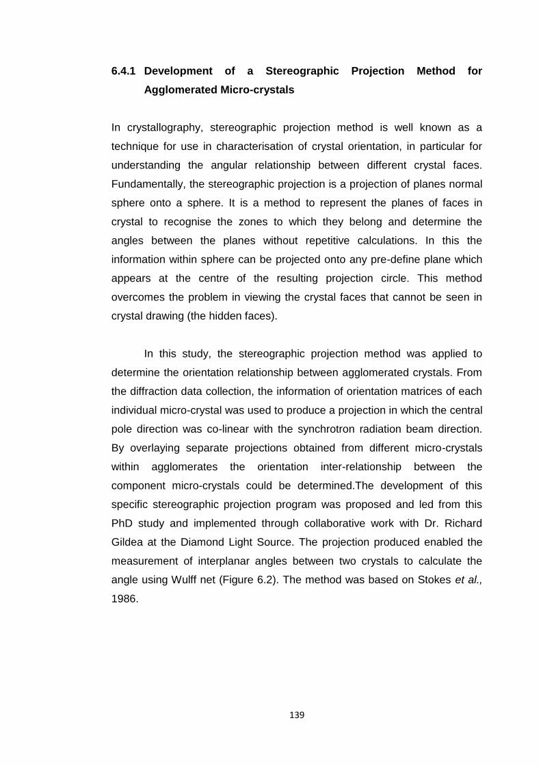
139

6.4.1 Development of a Stereographic Projection Method for

Agglomerated Micro-crystals

In crystallography, stereographic projection method is well known as a

technique for use in characterisation of crystal orientation, in particular for

understanding the angular relationship between different crystal faces.

Fundamentally, the stereographic projection is a projection of planes normal

sphere onto a sphere. It is a method to represent the planes of faces in

crystal to recognise the zones to which they belong and determine the

angles between the planes without repetitive calculations. In this the

information within sphere can be projected onto any pre-define plane which

appears at the centre of the resulting projection circle. This method

overcomes the problem in viewing the crystal faces that cannot be seen in

crystal drawing (the hidden faces).

In this study, the stereographic projection method was applied to

determine the orientation relationship between agglomerated crystals. From

the diffraction data collection, the information of orientation matrices of each

individual micro-crystal was used to produce a projection in which the central

pole direction was co-linear with the synchrotron radiation beam direction.

By overlaying separate projections obtained from different micro-crystals

within agglomerates the orientation inter-relationship between the

component micro-crystals could be determined.The development of this

specific stereographic projection program was proposed and led from this

PhD study and implemented through collaborative work with Dr. Richard

Gildea at the Diamond Light Source. The projection produced enabled the

measurement of interplanar angles between two crystals to calculate the

angle using Wulff net (Figure 6.2). The method was based on Stokes et al.,

1986.

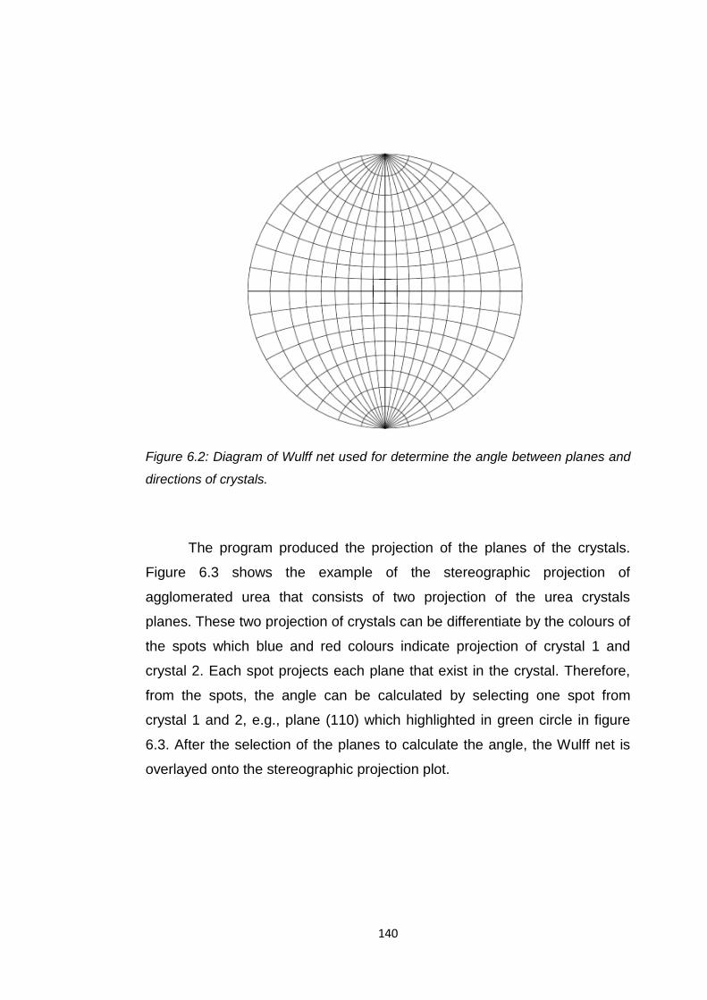
140

Figure 6.2: Diagram of Wulff net used for determine the angle between planes and

directions of crystals.

The program produced the projection of the planes of the crystals.

Figure 6.3 shows the example of the stereographic projection of

agglomerated urea that consists of two projection of the urea crystals

planes. These two projection of crystals can be differentiate by the colours of

the spots which blue and red colours indicate projection of crystal 1 and

crystal 2. Each spot projects each plane that exist in the crystal. Therefore,

from the spots, the angle can be calculated by selecting one spot from

crystal 1 and 2, e.g., plane (110) which highlighted in green circle in figure

6.3. After the selection of the planes to calculate the angle, the Wulff net is

overlayed onto the stereographic projection plot.

141

Figure 6.3: Example of stereographic projection result on agglomerated urea

crystals. Blue and red spots indicate the projected plane for crystal 1 and 2. Green

circles around the (110) plane of both crystals are selected planes to be used to

calculate the angle between planes.

The Wulff net is rotated until the both two planes aligned at the great circle,

as shown in figure 6.4. The space between line of the great circle is 10o.

Therefore, the angle between plane (110) crystal 1 and (110) crystal 2 is

110o.

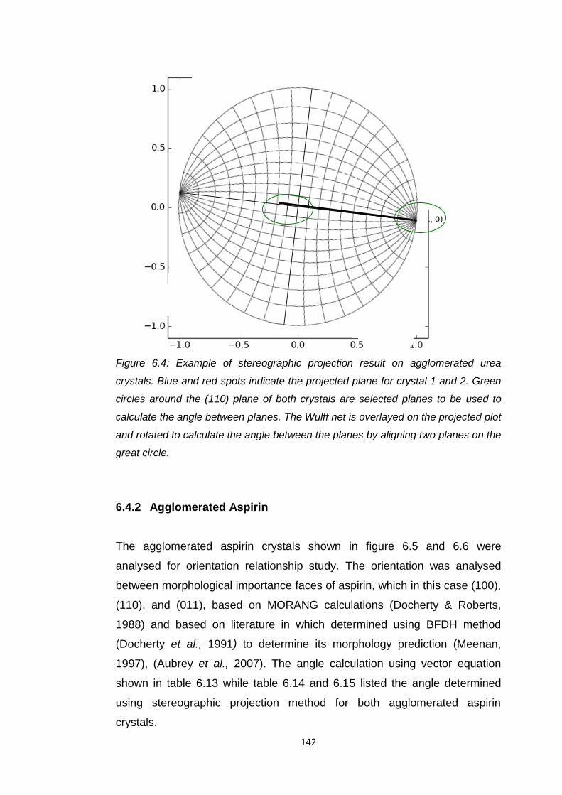
142

Figure 6.4: Example of stereographic projection result on agglomerated urea

crystals. Blue and red spots indicate the projected plane for crystal 1 and 2. Green

circles around the (110) plane of both crystals are selected planes to be used to

calculate the angle between planes. The Wulff net is overlayed on the projected plot

and rotated to calculate the angle between the planes by aligning two planes on the

great circle.

6.4.2 Agglomerated Aspirin

The agglomerated aspirin crystals shown in figure 6.5 and 6.6 were

analysed for orientation relationship study. The orientation was analysed

between morphological importance faces of aspirin, which in this case (100),

(110), and (011), based on MORANG calculations (Docherty & Roberts,

1988) and based on literature in which determined using BFDH method

(Docherty et al., 1991) to determine its morphology prediction (Meenan,

1997), (Aubrey et al., 2007). The angle calculation using vector equation

shown in table 6.13 while table 6.14 and 6.15 listed the angle determined

using stereographic projection method for both agglomerated aspirin

crystals.

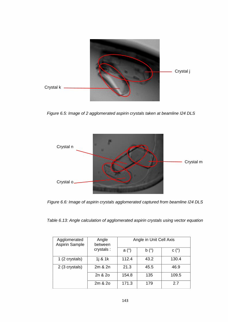
143

Figure 6.5: Image of 2 agglomerated aspirin crystals taken at beamline I24 DLS

Figure 6.6: Image of aspirin crystals agglomerated captured from beamline I24 DLS

Table 6.13: Angle calculation of agglomerated aspirin crystals using vector equation

Agglomerated Aspirin Sample

Angle between crystals :

Angle in Unit Cell Axis

a (°) b (°) c (°)

1 (2 crystals) 1j & 1k 112.4 43.2 130.4

2 (3 crystals) 2m & 2n 21.3 45.5 46.9

2n & 2o 154.8 135 109.5

2m & 2o 171.3 179 2.7

Crystal j

Crystal k

Crystal n

Crystal o

Crystal m

144

Table 6.14: Angle determination using stereographic projection method of

agglomerated aspirin (sample 1)

Figure 6.7: Stereographic projection plots of agglomerated aspirin crystals sample

no.1: (sample j and k)

Planes for crystals 1

(angle, θ (o)) j k

(1 0 0) (1 0 0) 68

(1 1 0) (1 1 0) 84

(0 1 1) (0 1 1) 70

(1 0 0) (1 1 0) 43

(0 1 1) (0 -1 1) 14

(-1 1 0) (-1 1 0) 10

145

Figure 6.8: Stereographic projection plots for aspirin crystals samples no.2: (sample

m & n)

Figure 6.9: Stereographic projection plots for aspirin crystals sample no.2: (sample

n and sample o)

146

Table 6.15: Angle determination using stereographic projection method of

agglomerated aspirin (sample 2)

In this section, first, the discussion is on comparison between the results

from vector equation calculations and stereographic projection method. To

compare between both methods, the (100) plane was chosen as it is from

the a-axes of table 6.13. The results from both showed the same angle

determined (68o) in which 112o equivalent to 68o. The smallest angle that

can be observed was between the (-110) planes which is 10o and between

the (011) planes which is 14o. In sample 2 (figure 6.6), which involves three

agglomerated aspirin crystals, the angles between crystals m-n, n-o, and m-

o were determined. The angle between m-o was determined just to

confirmed the angles obtained agree with the image in figure 6.5 that show

the parallelism of the crystals gives very small angle values ((100), (110) and

(011) planes) shown in table 6.15. Figure 6.10 shows the predicted

morphology of aspirin based on attachment energy model (Hammond et al.,

Planes for crystals 2

(angle, θ (o))

m n o

(1 0 0) (1 0 0)

18

(1 1 0) (1 1 0) 47

(0 1 1) (0 1 1) 132

(1 0 0) (1 1 0) 58

(0 -1 1) (0 1 1) 22

(-1 1 0) (-1 1 0) 32

(1 0 0) (1 0 0) 16

(1 1 0) (1 1 0) 44

(0 1 1) (0 1 1) 20

(1 0 0) (1 1 0) 74

(0 -1 1) (0 1 1) 42

(-1 1 0) (-1 1 0) 32

(1 0 0)

(1 0 0) 2

(1 1 0) (1 1 0) 2

(0 1 1) (0 -1 1) 2

(1 0 0) (1 1 0) 60

(-1 1 0) (-1 1 0) 2

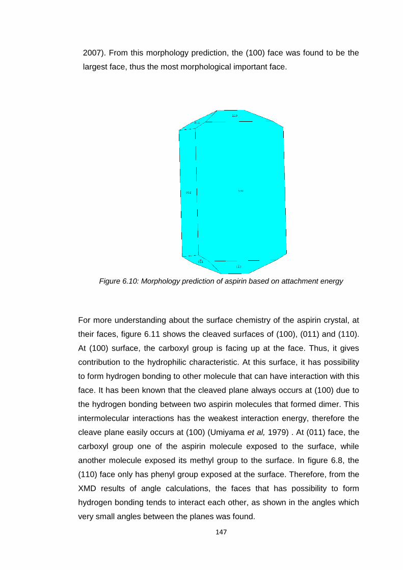
147

2007). From this morphology prediction, the (100) face was found to be the

largest face, thus the most morphological important face.

Figure 6.10: Morphology prediction of aspirin based on attachment energy

For more understanding about the surface chemistry of the aspirin crystal, at

their faces, figure 6.11 shows the cleaved surfaces of (100), (011) and (110).

At (100) surface, the carboxyl group is facing up at the face. Thus, it gives

contribution to the hydrophilic characteristic. At this surface, it has possibility

to form hydrogen bonding to other molecule that can have interaction with this

face. It has been known that the cleaved plane always occurs at (100) due to

the hydrogen bonding between two aspirin molecules that formed dimer. This

intermolecular interactions has the weakest interaction energy, therefore the

cleave plane easily occurs at (100) (Umiyama et al, 1979) . At (011) face, the

carboxyl group one of the aspirin molecule exposed to the surface, while

another molecule exposed its methyl group to the surface. In figure 6.8, the

(110) face only has phenyl group exposed at the surface. Therefore, from the

XMD results of angle calculations, the faces that has possibility to form

hydrogen bonding tends to interact each other, as shown in the angles which

very small angles between the planes was found.

148

(a) (b)

(c)

Figure 6.11: The cleave surfaces of aspirin at (a) (100), (b) (110), and (c) (001)

6.4.3 Agglomerated unmodified urea and urea modified by biuret as

prepared at different cooling rates

In this section, the agglomerated unmodified urea and urea modified by

biuret were analysed for orientation relationship between the agglomerated

component micro-crystals. The results for angle calculated using vector

equation and stereographic projection method was tabulated in table 6.16 to

6.25.

Table 6.16 and 6.17 show the values of angles for unmodified urea

and urea modified by biuret recrystallised at 0.1oC/min. Figure 6.12 shows

the image of sample no.5 as stated in table 6.16 and 6.17 for the

agglomerated unmodified urea crystals together with the stereographic

149

projection plots for the agglomerates. Images for sample no.1 to sample

no.4 are attached in the appendix as Figure 1 to 4.

Table 6.16: Angle calculations between agglomerated unmodified urea 0.1oC/min

using vector equation

Agglomerated Urea Sample

No.



a (°) b (°) c (°)

1 (2 crystals) 1p & 1q 69.2 93.2 35.3

2 (2 crystals) 2p & 2q 44.4 102.8 (77.2) 82.2

3 (2 crystals) 3p & 3q 65.3 82.0 60.0

4 (2 crystals) 4p & 4q 53 50.1 24.3

5 (2 crystals) 5p & 5q 1.8 1.2 1.3


using stereographic projection

Planes for crystals angle, θ (o) for samples:

P q 1 2 3 4 5

(0 0 1) (0 0 1) 36 82 60 154 (26) 0

(1 1 0) (1 1 0) 32 74 88 44 0

(0 0 1) (1 1 0) 63 68 34 66 90

(1 1 1) (1 1 1) 120 95 66 30 0

(1 1 1) (1 1 0) 83 64 54 36 40

(0 0 1) (1 1 1) 100 69 16 26 50

The values of angles in table 6.17 were determined from the stereographic

plots by using the Wulff net to determine the orientation angles between two

crystals. Sample no.5 gives the significant interest as the value of the angles

shows the parallelism between the crystals.

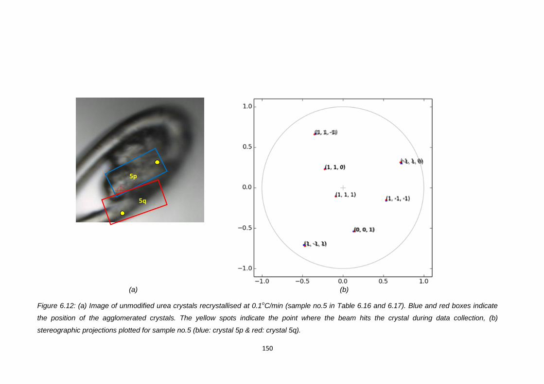
150

(a) (b)

Figure 6.12: (a) Image of unmodified urea crystals recrystallised at 0.1oC/min (sample no.5 in Table 6.16 and 6.17). Blue and red boxes indicate

the position of the agglomerated crystals. The yellow spots indicate the point where the beam hits the crystal during data collection, (b)

stereographic projections plotted for sample no.5 (blue: crystal 5p & red: crystal 5q).

5p

5q

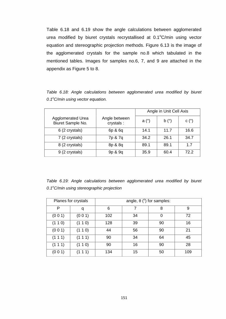
151

Table 6.18 and 6.19 show the angle calculations between agglomerated

urea modified by biuret crystals recrystallised at 0.1oC/min using vector

equation and stereographic projection methods. Figure 6.13 is the image of

the agglomerated crystals for the sample no.8 which tabulated in the

mentioned tables. Images for samples no.6, 7, and 9 are attached in the

appendix as Figure 5 to 8.

Table 6.18: Angle calculations between agglomerated urea modified by biuret

0.1oC/min using vector equation.

Table 6.19: Angle calculations between agglomerated urea modified by biuret

0.1oC/min using stereographic projection

Agglomerated Urea Biuret Sample No.



a (°) b (°) c (°)

6 (2 crystals) 6p & 6q 14.1 11.7 16.6

7 (2 crystals) 7p & 7q 34.2 26.1 34.7

8 (2 crystals) 8p & 8q 89.1 89.1 1.7

9 (2 crystals) 9p & 9q 35.9 60.4 72.2


P q 6 7 8 9

(0 0 1) (0 0 1) 102 34 0 72

(1 1 0) (1 1 0) 128 39 90 16

(0 0 1) (1 1 0) 44 56 90 21

(1 1 1) (1 1 1) 90 34 64 45

(1 1 1) (1 1 0) 90 16 90 28

(0 0 1) (1 1 1) 134 15 50 109

152

(a) (b)

Figure 6.13: (a) Image of urea modified by biuret crystals recrystallised at 0.1oC/min (sample no.8 in Table 6.18 and 6.19) Blue and

red boxes indicate the position of the agglomerated crystals. Yellow spots indicate the point where the beam hits the crystal during

data collection, (b) stereographic projections plotted for sample no.8 (blue: crystal 8p & red: crystal 8q).

8p

8q

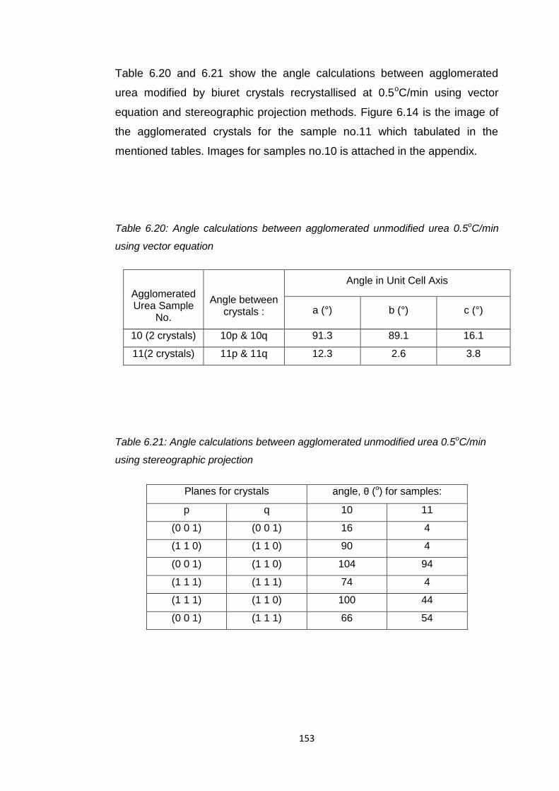
153


urea modified by biuret crystals recrystallised at 0.5oC/min using vector

equation and stereographic projection methods. Figure 6.14 is the image of

the agglomerated crystals for the sample no.11 which tabulated in the

mentioned tables. Images for samples no.10 is attached in the appendix.






No.



a (°) b (°) c (°)

10 (2 crystals) 10p & 10q 91.3 89.1 16.1

11(2 crystals) 11p & 11q 12.3 2.6 3.8


p q 10 11

(0 0 1) (0 0 1) 16 4

(1 1 0) (1 1 0) 90 4

(0 0 1) (1 1 0) 104 94

(1 1 1) (1 1 1) 74 4

(1 1 1) (1 1 0) 100 44

(0 0 1) (1 1 1) 66 54

154

(a) (b)

Figure 6.14: (a) Image of unmodified urea crystals recrystallised at 0.5oC/min (sample no.11 in Table 6.20 and 6.21). Blue and red

boxes indicate the position of the agglomerated crystals. The yellow spots indicate the point where the beam hits the crystal during


11p

11q

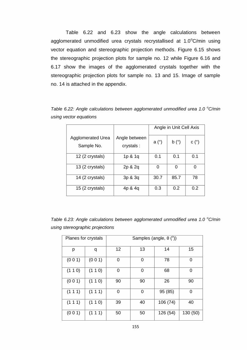
155

Table 6.22 and 6.23 show the angle calculations between

agglomerated unmodified urea crystals recrystallised at 1.0oC/min using

vector equation and stereographic projection methods. Figure 6.15 shows

the stereographic projection plots for sample no. 12 while Figure 6.16 and

6.17 show the images of the agglomerated crystals together with the

stereographic projection plots for sample no. 13 and 15. Image of sample

no. 14 is attached in the appendix.

Table 6.22: Angle calculations between agglomerated unmodified urea 1.0 oC/min

using vector equations

Agglomerated Urea

Sample No.

Angle between

crystals :


a (°) b (°) c (°)

12 (2 crystals) 1p & 1q 0.1 0.1 0.1

13 (2 crystals) 2p & 2q 0 0 0

14 (2 crystals) 3p & 3q 30.7 85.7 78

15 (2 crystals) 4p & 4q 0.3 0.2 0.2

Table 6.23: Angle calculations between agglomerated unmodified urea 1.0 oC/min

using stereographic projections

Planes for crystals Samples (angle, θ (o))

p q 12 13 14 15

(0 0 1) (0 0 1) 0 0 78 0

(1 1 0) (1 1 0) 0 0 68 0

(0 0 1) (1 1 0) 90 90 26 90

(1 1 1) (1 1 1) 0 0 95 (85) 0

(1 1 1) (1 1 0) 39 40 106 (74) 40

(0 0 1) (1 1 1) 50 50 126 (54) 130 (50)

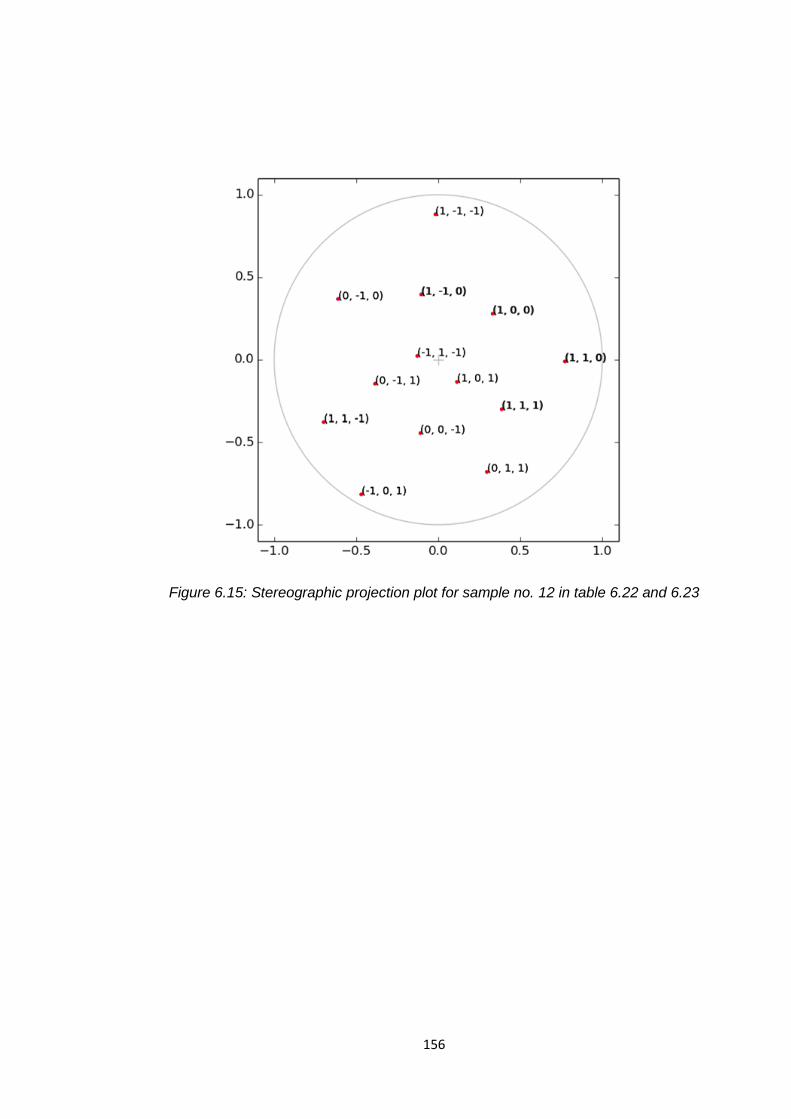
156

Figure 6.15: Stereographic projection plot for sample no. 12 in table 6.22 and 6.23

157

(a) (b)

Figure 6.16: (a) Image of unmodified urea crystals recrystallised at 1.0oC/min (sample no.13 in Table 6.22 and 6.23). Blue and red boxes

indicate the position of the agglomerated crystals. The yellow spots indicate the point where the beam hits the crystal during data

collection, (b) stereographic projections plotted for sample no.13 (blue: crystal 13p & red: crystal 13q). Blue dots cannot be seen in the

plotted image because the plots overlapped with the red dots plotted.

13p

13q

158

(a) (b)

Figure 6.17: (a) Image of unmodified urea crystals recrystallised at 1.0oC/min (sample no.15 in Table 6.22 and 6.23). Blue and red

boxes indicate the position of the agglomerated crystals. The yellow spots indicate the point where the beam hits the crystal during

data collection, (b) stereographic projections plotted for sample no.15 (blue: crystal 15p & red: crystal 15q). The blue dots cannot be

seen in the plotted image because the plots overlapped with red dots plots.

15p 15q

159


unmodified urea crystals recrystallised at 1.0oC/min using vector equation

and stereographic projection methods. Figure 6.18 shows the image of the

agglomerated crystals together with the stereographic projection plots for

sample no.17. Image for sample no. 16 is attached in the appendix.

Table 6.24: Angle calculations between agglomerated urea modified by biuret 1.0

oC/min using vector equation

Agglomerated Urea-biuret Sample No.



a (°) b (°) c (°)

16 (2 crystals) 1p & 1q 91.3 91 51.1

17 (2 crystals) 2p & 2q 78.4 79.4 11

Table 6.25: Angle calculations between agglomerated urea modified by biuret 1.0

oC/min using stereographic projection


p q 16 17

(0 0 1) (0 0 1) 130 (50) 12

(1 1 0) (1 1 0) 80 80

(0 0 1) (1 1 0) 56 94

(1 1 1) (1 1 1) (100) (80) 54

(1 1 1) (1 1 0) 112 (68) 86

(0 0 1) (1 1 1) 90 54

160

(a) (b)

Figure 6.18: (a) Image of urea modified by biuret crystals recrystallised at 1.0oC/min (sample no.17 in Table 6.24 and 6.25). Blue and

red boxes indicate the position of the agglomerated crystals. The yellow spots indicate the point where the beam hits the crystal during


17p

17q

161

In stereographic projection analysis, angle between planes were

determined. The angles values of agglomerated unmodified urea and

modified urea by biuret crystals were compared. First, this work is discussed

on the validation of the angle calculations using vector equation and using

stereographic projection method. Three planes were chosen which {100}, {0-

10} and {00-1} from stereographic projection plots. This is to compare the

values obtained from the vector calculations in which it calculates the angle

between planes by the vector of a- , b- and c- axes with the angles values

determined by streographic projection method. From all the values obtained,

it is confirmed that the values are same and validate the results. To explain

clearly the orientation relationship between the agglomerated crystals, the

planes that were chosen to determine the relationship are listed in table

6.26. There are many planes that can be used to determine the angles

between crystals plane, however, to simplify it; those planes in table 6.26

were chosen.

Table 6.26: Planes use for angle calculations determination

Planes for crystals

p q

(0 0 1) (0 0 1)

(1 1 0) (1 1 0)

(0 0 1) (1 1 0)

(1 1 1) (1 1 1)

(1 1 1) (1 1 0)

(0 0 1) (1 1 1)

162

Table 6.27 summarises the angle determination of the agglomerated urea

crystals.

Table 6.27: Summary of angle calculations of the agglomerated unmodified urea

and urea modified by biuret crystals. The samples summarised are chosen based

on the smallest angle value to show the parallelism between crystals.

*Actual angle between planes calculated by using MORANG program

In this study, the comparison between the same crystals in the same

batch, for example five samples of unmodified urea crystallised at 0.1oC/min

in table 6.16 and 6.17 showed the values of the angles were in random

numbers. The same results for unmodified urea crystals at other cooling

rates, and urea modified urea by biuret crystals. However, there were seven

samples that show they are parallel to each other (as shown in table 6.27).

The samples number 5, 8, 12, 13 and 15 show the perfect parallelism

occurred between two agglomerates urea crystals. Samples number 11 and

17 are slightly misoriented for small degrees. Overall, these seven results

from the agglomerated urea crystals show the crystals are aligned to each

other. The results show good example of preferred orientation with parallel

agglomeration. Outside this experiment, the observation on agglomeration of

Planes

*Actual

angle

between

planes

Samples (o)

5 8 11 12 13 15 17

(0 0 1) (0 0 1) 0 0 0 4 0 0 0 12

(1 1 0) (1 1 0) 0 0 0 4 0 0 0 80

(0 0 1) (1 1 0) 90 90 90 94 90 90 90 94

(1 1 1) (1 1 1) 0 0 64 4 0 0 0 54

(1 1 1) (1 1 0) 40 40 40 44 39 40 40 86

(0 0 1) (1 1 1) 50 50 50 54 50 50 50 54

163

urea crystals under microscope showed that the agglomerated urea crystals

are mostly parallel and align to each other, either parallel at the same

orientation or at opposite direction. This perhaps reflects the epitaxial nature

of the growth process for many crystals (Chemla, 2012). In general, the

epitaxy growth occurs by forming a new layer film on top of the growing

surface. In the case of urea, the epitaxy growth occurs on the same

metarials known as homoepitaxy. It shows the epitaxially grown crystals that

occur at its {110} interface. It is could be because of the fastest growth

occurs at [001] direction, therefore the epitaxial growth selectively occurs at

the most stable growing face which is {110} form. It is apparently the crystals

grown in parallel to each other during crystal growth, regardless the crystals

growth at different conditions of cooling rates and with the impurities. The

surface chemistry of urea has been explained in detail in chapter 5 in

molecular modelling section.

In both cases, aspirin and urea agglomerates, the results confirmed

that the angles obtained from vector calculations and stereographic

projections agreed each other with additional proof by observing the

agglomerates micro-crystals samples images that the angles determined are

similar to the orientation of the crystals in the images. In this study, the

application of stereographic projection in crystallography, specifically the

combination of it with the information obtained from X-ray diffraction data

can be a platform to understand the relationship between agglomerated

particles. As the basic application of this method is to determine the angular

relationships within one crystal faces, it had been applied to determine the

relationships between twinning planes of twinned crystal (Dechamps et al,

2000), and understand defects occur in crystal (Salje, 1995). From this

study, the relationships of homoepitaxy growth on agglomerates micro-

crystals can be understood and helps to further use of the stereographic

projection.

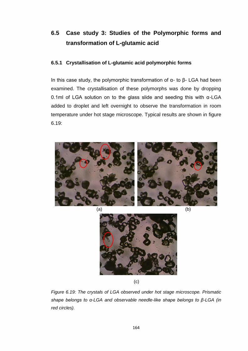
164

6.5 Case study 3: Studies of the Polymorphic forms and

transformation of L-glutamic acid

6.5.1 Crystallisation of L-glutamic acid polymorphic forms

In this case study, the polymorphic transformation of α- to β- LGA had been

examined. The crystallisation of these polymorphs was done by dropping

0.1ml of LGA solution on to the glass slide and seeding this with α-LGA

added to droplet and left overnight to observe the transformation in room

temperature under hot stage microscope. Typical results are shown in figure

6.19:

(a) (b)

(c)

Figure 6.19: The crystals of LGA observed under hot stage microscope. Prismatic

shape belongs to α-LGA and observable needle-like shape belongs to β-LGA (in

red circles).

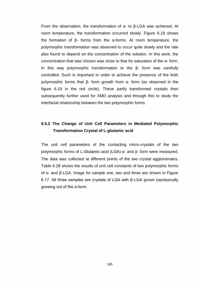
165

From the observation, the transformation of α- to β-LGA was achieved. At

room temperature, the transformation occurred slowly. Figure 6.19 shows

the formation of β- forms from the α-forms. At room temperature, the

polymorphic transformation was observed to occur quite slowly and the rate

also found to depend on the concentration of the solution. In this work, the

concentration that was chosen was close to that for saturation of the α- form.

In this way polymorphic transformation to the β- form was carefully

controlled. Such is important in order to achieve the presence of the both

polymorphic forms that β- form growth from α- form (as observed in the

figure 6.19 in the red circle). These partly transformed crystals then

subsequently further used for XMD analysis and through this to study the

interfacial relationship between the two polymorphic forms.

6.5.2 The Change of Unit Cell Parameters in Mediated Polymorphic

Transformation Crystal of L-glutamic acid

The unit cell parameters of the contacting micro-crystals of the two

polymorphic forms of L-Glutamic acid (LGA) α- and β- form were measured.

The data was collected at different points of the two crystal agglomerates.

Table 6.28 shows the results of unit cell constants of two polymorphic forms

of α- and β-LGA. Image for sample one, two and three are shown in Figure

6.17. All three samples are crystals of LGA with β-LGA grown topotaxically

growing out of the α-form.

166

(a) (b)

(c)

Figure 6.20: Samples of LGA with β – crystal grows from α-LGA. The arrow pointed

on the point of the beam hits the interface: (a) sample 1, (b) sample 2, (c)sample 3.

Beam hits at the

interface

Beam hits at the interface

Beam hits at the interface

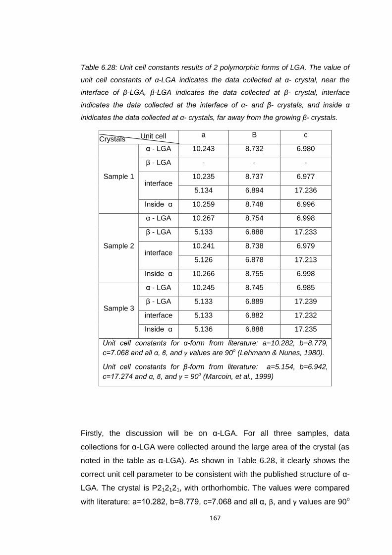
167

Table 6.28: Unit cell constants results of 2 polymorphic forms of LGA. The value of

unit cell constants of α-LGA indicates the data collected at α- crystal, near the

interface of β-LGA, β-LGA indicates the data collected at β- crystal, interface

indicates the data collected at the interface of α- and β- crystals, and inside α

inidicates the data collected at α- crystals, far away from the growing β- crystals.

Firstly, the discussion will be on α-LGA. For all three samples, data

collections for α-LGA were collected around the large area of the crystal (as

noted in the table as α-LGA). As shown in Table 6.28, it clearly shows the

correct unit cell parameter to be consistent with the published structure of α-

LGA. The crystal is P212121, with orthorhombic. The values were compared

with literature: a=10.282, b=8.779, c=7.068 and all α, β, and γ values are 90o

a B c

Sample 1

α - LGA 10.243 8.732 6.980

β - LGA - - -

interface 10.235 8.737 6.977

5.134 6.894 17.236

Inside α 10.259 8.748 6.996

Sample 2

α - LGA 10.267 8.754 6.998

β - LGA 5.133 6.888 17.233

interface 10.241 8.738 6.979

5.126 6.878 17.213

Inside α 10.266 8.755 6.998

Sample 3

α - LGA 10.245 8.745 6.985

β - LGA 5.133 6.889 17.239

interface 5.133 6.882 17.232

Inside α 5.136 6.888 17.235

Unit cell constants for α-form from literature: a=10.282, b=8.779,

c=7.068 and all α, β, and γ values are 90o (Lehmann & Nunes, 1980).

Unit cell constants for β-form from literature: a=5.154, b=6.942,

c=17.274 and α, β, and γ = 90o (Marcoin, et al., 1999)

Unit cell

(A°) Crystals

168

(Lehmann & Nunes, 1980). A slight difference with respect to the literature

was observed associated with a percentage difference of 0.4%, 0.8%, and

1% for each a, b, and c values, respectively. Data collection at inside α-LGA

means the data area of data was being collected close to the interface, but

still in area of α-form. For this area, the values obtained are expected to

have lattice parameter of α-form for sample 1 and 2. However, sample 3

gives value of lattice parameter of β form. The explanation for this is that

perhaps because of the area is closed to the interface, in which the β-form

started to grow; therefore, it may already to have arrangement of β-form. For

data collection at β-form crystal, the beam hit the tip of the crystal. However,

the result for sample 1 of β-LGA could not be determined as it failed to be

indexed, thus further data processing could not proceed. The reason for this

failure in indexing was not clear but this may reflect the fact that the β-LGA

did not grow perfectly as β, therefore, the reflection data obtained has some

incorrect mapping from the diffraction spot. The other two samples give

consistent lattice parameters of β-LGA, which are a=5.154, b=6.942,

c=17.274 and α, β, and γ = 90o (Marcoin, et al., 1999). The percentage

variation for published data was 0.4%, 0.7%, and 0.2% for a, b, and c values

respectively.

6.5.3 Angle calculations between the contacting two polymorphs

resulting from the transformation between α- and β-forms of

LGA

The orientation relationship between polymorphic transformations of α- to β-

LGA was determined using both vector equation and stereographic

projection methods. Two samples of LGA crystals were used for analysis.

The important faces were selected in this study are {001}, {101}, and {111}

of α-form and {101}, {020}, and {021} of β-form (Hammond, et al., 2007).

The results for both methods are tabulated in the Table 6.29 and 6.30:

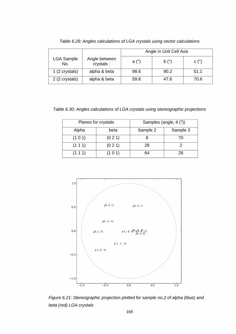
169

Table 6.29: Angles calculations of LGA crystals using vector calculations

LGA Sample No.



a (°) b (°) c (°)

1 (2 crystals) alpha & beta 98.6 90.2 51.1

2 (2 crystals) alpha & beta 59.8 47.6 70.6

Table 6.30: Angles calculations of LGA crystals using stereographic projections

Figure 6.21: Stereographic projection plotted for sample no.2 of alpha (blue) and

beta (red) LGA crystals


Alpha beta Sample 2 Sample 3

(1 0 1) (0 2 1) 8 70

(1 1 1) (0 2 1) 28 2

(1 1 1) (1 0 1) 64 26

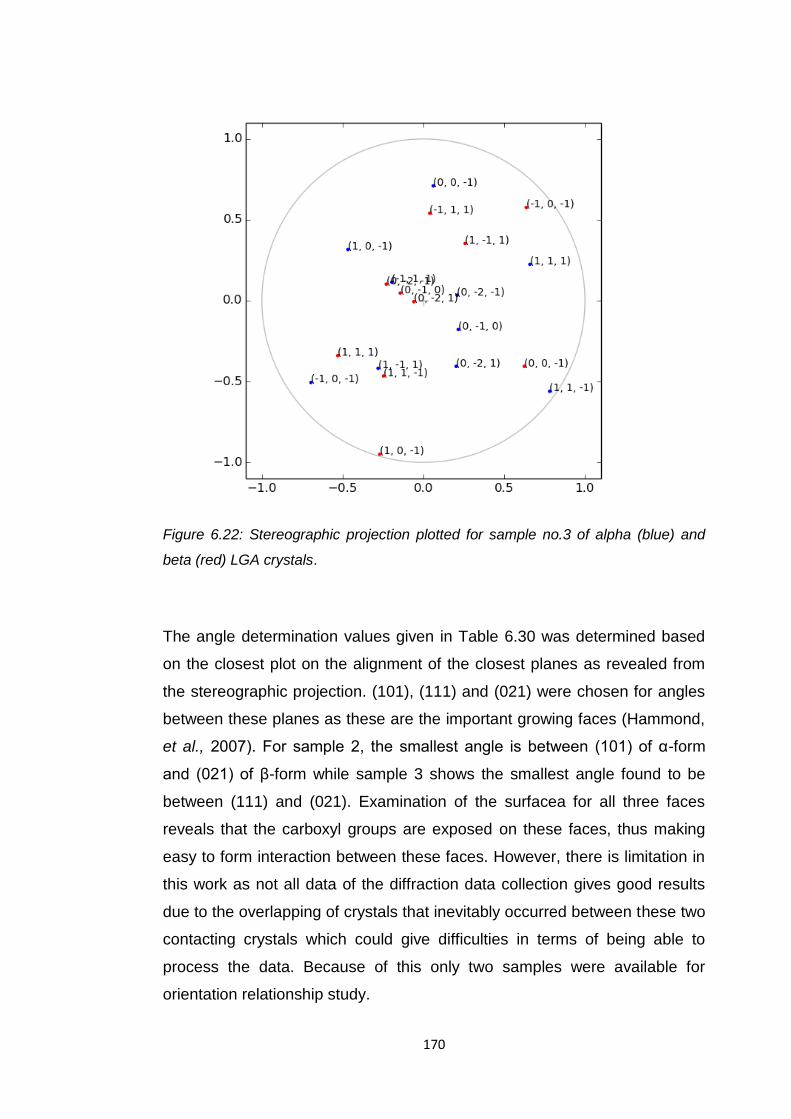
170

Figure 6.22: Stereographic projection plotted for sample no.3 of alpha (blue) and

beta (red) LGA crystals.

The angle determination values given in Table 6.30 was determined based

on the closest plot on the alignment of the closest planes as revealed from

the stereographic projection. (101), (111) and (021) were chosen for angles

between these planes as these are the important growing faces (Hammond,

et al., 2007). For sample 2, the smallest angle is between (101) of α-form

and (021) of β-form while sample 3 shows the smallest angle found to be

between (111) and (021). Examination of the surfacea for all three faces

reveals that the carboxyl groups are exposed on these faces, thus making

easy to form interaction between these faces. However, there is limitation in

this work as not all data of the diffraction data collection gives good results

due to the overlapping of crystals that inevitably occurred between these two

contacting crystals which could give difficulties in terms of being able to

process the data. Because of this only two samples were available for

orientation relationship study.

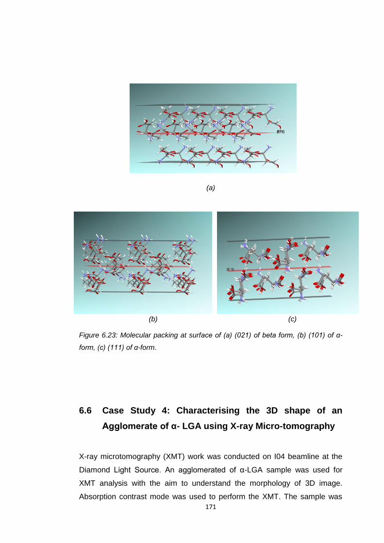
171

(a)

(b) (c)

Figure 6.23: Molecular packing at surface of (a) (021) of beta form, (b) (101) of α-

form, (c) (111) of α-form.

6.6 Case Study 4: Characterising the 3D shape of an

Agglomerate of α- LGA using X-ray Micro-tomography

X-ray microtomography (XMT) work was conducted on I04 beamline at the

Diamond Light Source. An agglomerated of α-LGA sample was used for

XMT analysis with the aim to understand the morphology of 3D image.

Absorption contrast mode was used to perform the XMT. The sample was

172

rotated between 0o to 180o for data collection to obtain the views of the

projection at different angle. One of the images of the beam showing the

projected sample image from the data collection is shown in Figure 6.24(a).

(a) (b)

(c)

Figure 6.24: Image of XMT data collection: (a) image of the beam with the sample

in, (b) flat field reference image, (c) image of the beam with sample after divided

each images in (a) with image in (b). The sample is circled in red.

Using the ImageJ software (Ferreira & Rasband, 2012), the raw data images

(example in Figure 6.24 (a)) were background substracted with respect to

the flat field reference image (Figure 6.24 (b)) i.e without sample to obtain

just the absorption contrast of the sample itself (Figure 6.24 (c)). This

process enables the acquisition of good quality images before the

reconstruction process was carried out. The flat field reference image is the

a b

173

image of field view without any sample exposed to the beam. Consistent

beam intensity is important to produce good quality image as if the beam

intensity were to change during the data collection period then good quality

images with high absorption contrast could not be obtained.

After obtaining flat field correction images, reconstruction process

was done using TomoJ software. In this process, the algorithms used were

alignment of the tilt series, determination of the tilt axis and application of the

ART (Algebraic Reconstruction Technique) using 10 iterations and a

relaxation coefficient of 0.1. Alignment of the tilt series was found to be

useful for shift and rotation correction of the images to produce good quality

of the reconstruction volume tomogram. The ART is a suitable technique to

be used to reconstruct tomography images for single particle analysis. A

detail about the method used is explained in Messaoudill et al., 2007. Figure

6.25 shows few slices of the reconstructed images.

Figure 6.25: The images cut into slices in z-direction during reconstruction.

From the set of slices from reconstruction results, the two dimensional

projections of the slice can be viewed as a full three-dimensional 3D image

through a process called volume rendering. The resultant 3D image of

agglomerated α-LGA sample so produced is shown in Figure 6.26.

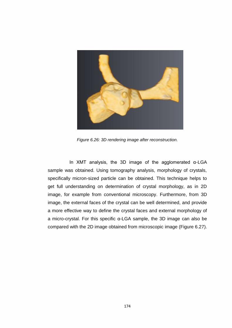
174

Figure 6.26: 3D rendering image after reconstruction.

In XMT analysis, the 3D image of the agglomerated α-LGA

sample was obtained. Using tomography analysis, morphology of crystals,

specifically micron-sized particle can be obtained. This technique helps to

get full understanding on determination of crystal morphology, as in 2D

image, for example from conventional microscopy. Furthermore, from 3D

image, the external faces of the crystal can be well determined, and provide

a more effective way to define the crystal faces and external morphology of

a micro-crystal. For this specific α-LGA sample, the 3D image can also be

compared with the 2D image obtained from microscopic image (Figure 6.27).

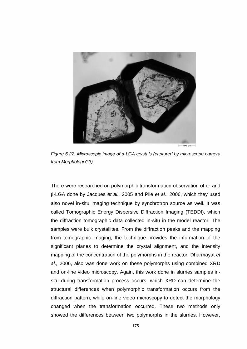
175

Figure 6.27: Microscopic image of α-LGA crystals (captured by microscope camera

from Morphologi G3).

There were researched on polymorphic transformation observation of α- and

β-LGA done by Jacques et al., 2005 and Pile et al., 2006, which they used

also novel in-situ imaging technique by synchrotron source as well. It was

called Tomographic Energy Dispersive Diffraction Imaging (TEDDI), which

the diffraction tomographic data collected in-situ in the model reactor. The

samples were bulk crystallites. From the diffraction peaks and the mapping

from tomographic imaging, the technique provides the information of the

significant planes to determine the crystal alignment, and the intensity

mapping of the concentration of the polymorphs in the reactor. Dharmayat et

al., 2006, also was done work on these polymorphs using combined XRD

and on-line video microscopy. Again, this work done in slurries samples in-

situ during transformation process occurs, which XRD can determine the

structural differences when polymorphic transformation occurs from the

diffraction pattern, while on-line video microscopy to detect the morphology

changed when the transformation occurred. These two methods only

showed the differences between two polymorphs in the slurries. However,

176

they were not be able to reveal the relationship in terms of how the

transformation occurs from α- to β-LGA. There have been also been

molecular modelling studies in which have attempted to show how this

transformation can occur and on what the specific faces. (Hammond, et al.

2007).

6.6.1 X-ray microdiffraction data of agglomerated α-LGA

The diffraction experiment was carried out on the two agglomerated α-LGA

shown in Figure 6.24 (as denoted a and b). Table 6.31 shows the routine

data in diffraction work which is the unit cell parameters determination. Table

6.32 presents the angle calculation results from vector calculation and

stereographic projection.

Table 6.31: Unit cell parameters determination of two agglomerated α-LGA

unit cell parameters a b c β

crystal j 6.996 8.758 10.265 90

crystal k 7.002 8.763 10.268 90

Table 6.32: Angle determination using vector calculations and stereographic

projection method

Angle calculation based on vector calculations


Angle in Unit Cell Axis (o)

a b c

a & b 14 6 49.344

Angle calculated from stereographic projection

Planes for crystals

Angle (o) a b

(101) (101) 80

(111) (111) 80

(101) (02-1) 28

177

Figure 6.28: Stereographic projection plots of two agglomerated α-LGA. Blue dots

represent crystal a and red dots represent crystal b.

The angle calculation results in table 6.32 of two agglomerated α-LGA is

compared between both methods. The results given in table 6.32 does not

give good agreement between both method. It is because in vector

calculation, it considers the three basic direction of unit cell axis, a,b,c, [100],

[010], and [001] while the important planes of the crystals (101), (111) and

(021). However, in this carried out experiment, the objective is to assess the

capability the combined method of X-ray microdiffraction and X-ray

microtomography. In this work, this is the only experiment that can be done

(-1,-1,-1) (-1,0,-1)

(0,-2,-1)

(0,0,1)

(-1,0,-1)

(0.,1,0)

(-1,-1,-1)

178

for the combined technique. It needs more analysis on different samples to

evaluate further the relationship between the agglomerated samples.

6.7 Discussion

In XMD and XMT works, the development of this methods gives

understanding in the surface properties of the inter-particles, particularly in

this study is agglomerated materials. The first attempt to do is the combined

technique of the XMD and XMT at the same microfocus beamline I24.

However, because of the stability of the beam for the tomography still under

development to achieve high stablility in order to produce good result of

imaging, the XMT only could be done on I04 macrocrystallography beamline.

Only one sample of agglomerated α-LGA was done for combined XMD and

XMT technique. However, further experiments need to be carried out in

order to get full understanding of the inter-particle relationships between the

agglomeration. In tomography imaging technique, the challenging issue is to

do with the absorption contrast in which as using micron-sized particles, the

absorption contrast plays the important roles to achieve the good quality

data. Further studies are clearly needed, notably using wavelength

dispersion technique to achieve the best tomographic contrast.

6.8 Closing Remarks

The approach of simultaneous X-ray microdiffraction and microtomography

experiments. These techniques offer promise for the study of micron-sized

particles and future improvement during data collection in order to produce

good quality results. By determination of orientation relationship between

agglomerates using XMD and the 3D imaging technique of XMT, the

understanding on molecular surface properties of crystals and the crystal

morphology from the 3D image can be achieved opening the way to a more

molecular centred science in terms of the agglomeration of micro-crystals.

179

References

1. Aubrey-Medendorp, C., Parkin, S., Li, T., (2007). The Confusion of

Indexing Aspirin Crystals. J. Pharm.Sci. (97) 1361-1367.

2. Chemla, D.S., (2012). Nonlinear Optical Properties of Organic

Molecules and Crystals. Vol.1. Academic Press, Inc., Orlando.

3. Dechamps, M., de Leon Guevara, A.M., Pinsard, L., Revcolevschi, A.,

(2000). Twinned microstructure of La1-X SrX MnO3 solid solutions,

Philosophical Magazine A: (80) 119-127.

4. Dharmayat, S., J. C. De Anda, et al., (2006). "Polymorphic

transformation of L-glutamic acid monitored using combined on-line

video microscopy and X-ray diffraction." J. Cryst. Growth. (294) 35-

40.

5. Docherty, R., Roberts, K.J., Dowty, E., (1988). MORANG-A Computer

Program Designed to Aid in the Determinations of Crystal

Morphology. Comput. Phys. Commun. (51) 423-430.

6. Docherty, R., Clydesdale, G., Roberts, K.J., Bennema, P., (1991).

Application of Bravais-Freidel-Donnay-Harker, Attachment Energy

and Ising Models to Predicting and Understanding the Morphology of

Molecular Crystals. J. Phys. D: Appl. Phys. (24) 89-99.

7. Evans, P.R., (1999). Some Notes on Choices in Data Collection. Acta

Crsytallogr. D (55): 1771-1772

8. Farrugia, L.J., (2012). WinGX and ORTEP for Windows: an update. J.

Appl. Crystallogr. (45):849-854.

9. Ferreira, T., Rasband, W., 2012. ImageJ User Guide (Revised

Edition).

10. Ferrari, E. S.; Davey, R. (2001). Solution-Mediated Transformation of

to L-glutamic acid: Rate Enhancement Due to Secondary Nucleation.

J. Cryst. Growth Des. (4) 1061.

180

11. Hammond, R. B., K. Pencheva, Robert, K.J,. (2007). "Molecular

modeling of crystal-crystal interactions between the alpha- and beta-

polymorphic forms of L-glutamic acid using grid-based methods." J.

Cryst. Growth Des. (7): 875-884.

12. Harrison, A. Ibberson, R., Robb, G., Whittaker, G., Wilson, C.,

Youngson, D. (2002). In-situ Neutron Diffraction Studies of Single

Crystals and Powders during Microwave Irradiation. Faraday Discuss.

(122) 363-379.

13. Kim, Y., Machida, K., Taga, T., (1985). Structure Determination and

Packing Analysis of Aspirin Crystal. Chem. Pharm. Bull. (33) 2641-

2647.

14. Lehmann, M.S., Nunes, A.C., (1980). A Short Hydrogen Bond

between Near Identical Carboxyl Groups in the α Modification of L-

Glutamic Acid. Acta Crystallogr. B. (36) 1621-1625.

15. Pile, K., X. Lai, et al., (2006). "An investigation of crystallite alignment

and polymorphic interaction of glutamic acid using an in situ

synchrotron X-ray diffraction tomographic technique." J. Cryst.

Growth. (294) 41-45.

16. Salje, E.K.H., (1995). A novel 7-circle diffractometer for the rapid

analysis of extended defects in thin films, single crystals, and

ceramics. Phase Transitions: A Multinational Journal. (55) 37-56.

17. Stokes, G.K., Keown, S.R., Dyson, D.J., (1968). The Construction of

Stereographic Projections by Computer. J. Appl. Crystallogr. (1) 68-

70.

18. Umiyama, H., Nakagawa, S., Moriguchi, I., (1979). Molecular Orbital

Study of the Cleavage of Aspirin Crystals. The J. Phys. Chem. (83)

2048-2052.

19. Wheatley, P.J., (1964). The Crystal and Molecular Structure of

Aspirin. J. Chem. Soc. 6036-6048.

181

CHAPTER VII

CONCLUSION & FUTURE WORKS

182

7.1 Introduction

In this chapter the main results are summarised in section 7.2 together with

a re-appraisal of the thesis aims and objectives in 7.3, as described in

section 1.2. The suggestion for future work is described in section 7.4.

7.2 Conclusion of this Study

This work included the bulk properties of the crystals, the internal atomic

information of the single micro-crystals, together with an understanding of

the external shape of the crystals, and molecular modelling analysis from the

crystal structure information. This thesis involved a combination of

experimental analysis carried out in the laboratory, molecular modelling

analysis and XMD and XMT studies at the synchrotron radiation source. The

research concluded that the bulk properties of crystalline powders can be

represented by their analysis at single micro-crystals level and that

correlation of the bulk powders and the single micro-crystals can be

understood by integrate these three analysis together.

7.2.1 Influence of Crystallisation Environment the Physico-chemical

Properties of Urea Crystals

Crystallisation of urea in 99% ethanol produced long needle-like crystals.

The addition of 4% of biuret modified the original morphology of urea from

this morphology to a more prismatic shape. The difference in cooling rates

for crystallisation was also found to affect the crystals size produced. At

lower cooling rates, larger crystals were produced whilst at higher cooling

rates, smaller sizes of crystals were produced. This is reflection of the higher

cooling rates where supersaturation is higher and hence the nucleation

occurs at a faster rate, therefore there is a greater number of the crystals

which do not grow to its some extent. The effect of biuret on urea

183

morphology and cooling rates effect was also studied using surface energy

analysis. From this study, the needle-like unmodified urea was found to have

a lower dispersive surface energy than the urea crystals modified by which

when modified by the presence of biuret. This is because when the crystals

become prismatic in shape, the fraction of the surface area of the {111}

faces increases with respect to that of the {110} faces. The small size of the

crystals prepared at higher cooling rates were also found to have higher

dispersive surface energy values than the larger size crystals, consistent

with the latter having larger surface area per volume. Therefore, increasing

surface area increased the numbers of surface energetic sites on the crystal

surface hence yielding a higher surface energy. Molecular modelling also

was carried out to validate the experimental results and the dispersive

surface energy of the particle was calculated from first principles based on

morphology predictions. In this, the face-specific surface energies were

weighted with respect to their fractional surface areas in the observed

morphologies. The resultant dispersive surface energies were found to give

good agreement with the experimental results. In the other experiment using

dynamic vapour sorption method to evaluate the adsorption of water on

unmodified urea and urea modified by biuret samples in order to observe the

effect of addition of biuret on the water adsorption on the urea samples, it

shows that at lower relative humidity, less than 70% RH, the water

adsorption on both samples are slow, but above this RH, the mass changed

increased rapidly, showing that the samples absorbed water rather than only

adsorption. However, the adsoprtion occurred faster in unmodified urea as

the large surface of hydrophilic {110} but, lower adsorption in urea modified

by biuret as the addition of biuret made the {110} shrunk, thus, less

hydrophilic surface, hence, lower adsoprtion can be seen.

7.2.2 XMD and XMT Studies of the Structure and Orientation of Single

Agglomerated Micro-crystals

This work demonstrated the capability of the microfocus synchrotron

radiation beamlines and facilities to measure the atomic arrangement of the

184

agglomerated micron- sized crystals (20-50µm). The analysed data showed

the variability of powdered samples of their unit cell parameters and the

crystal perfection. This was done by using XMD technique. Using XMT, it

was demonstrated that of micro-crystal agglomeration the 3-dimensional

imaging can be obtained to demonstrating that the interfaces between

agglomerated particles can be characterised. However, as the absorption

contrast is the limitation in this study, it needs more improvement in the

absorption contrast, for example the distance between sample and the

detector, and the wavelength used for future study.

7.3 Re-appraisal of Thesis Objectives

The main objective of this PhD work is to understand the surface properties

of micro-crystalline particles with the effect of process conditions such as

impurities and cooling rate to the crystal size and shape using surface

analysis methods and synchrotron radiation source to study the relative

orientation of the agglomerated micro-crystals. Molecular modelling analysis

used to correlate the bulk properties of powdered samples and the single

crystals. The examination on crystal size and shape produced at different

process conditions has successfully done by experimental analysis. The

study on the micro-crystals samples on XMD and XMT has several

limitations in which these techniques only available at the synchrotron

radiation source facilities, there was a limit in collecting enough data to be

analysed. The combined technique of XMD and XMT also still in

development stage. However, the results obtained in this PhD work using

these techniques shows a good start to continue for the combined

technique. However, it is a challenging work to correlate between bulk

crystalline powder samples with single particles. There is no direct method to

correlate between samples, powder and single particles. As mentioned in

above statement, the objective of this research is to understand the surface

properties of micro-particles with the effect of the additive. Therefore, the

surface energy analysis using inverse gas chromatography correlates

particle characterisation using Morphologi G3 together with molecular

185

modelling. Also, the correlation between inter-particle analysis on

agglomerates need to be work together with stereographic projection

method and molecular modelling. Nevertheless, more future works need to

be done to make this research become clearer to be understood.

7.4 Suggestion for Future Work

There are several recommendations for the extensive study from this work

that should be considered:

Crystallisation of urea at different process conditions, such as

different types of solvents to be used for crystallisation to observe the

morphological changes of urea and different percentage of impurities

to observe whether there is any changes could occur.

The robotic automatic handling for mounting micro-crystals is being

developed. Therefore, it could be used for future work for

understanding different micro-crystals type. The robotic handling also

can reduce time consume when selecting the crystals to be mounted

for data collection.

As agglomerated micro-crystals are the same type of materials stack

together, the phase contrast is low. Therefore it is recommended to

improve the absorption contrast of the XMT work in order to produce

high quality 3D tomography image.

The combined technique of XMD and XMT to be carried out for more

samples for repeatability and concise results. Therefore, if more

samples and data can be obtained, clear analysis can be done.

Futher work on molecular modelling such as using other modeliing

method (such as Systematic Search method) to evaluate the

molecule to surface interactions.

186

APPENDIX

xxviii

(a) (b)

Figure 1: (a) Image of unmodified urea crystals recrystallised at 0.1oC/min (sample no.1 in table 6.16 and 6.17 in page 148 and 149) (b)

stereographic projections plotted for sample no.1 (blue: crystal 1p & red: crystal 1q)

1q

1p

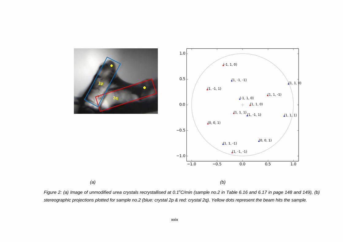
xxix

(a) (b)

Figure 2: (a) Image of unmodified urea crystals recrystallised at 0.1oC/min (sample no.2 in Table 6.16 and 6.17 in page 148 and 149), (b)

stereographic projections plotted for sample no.2 (blue: crystal 2p & red: crystal 2q). Yellow dots represent the beam hits the sample.

2p

2q

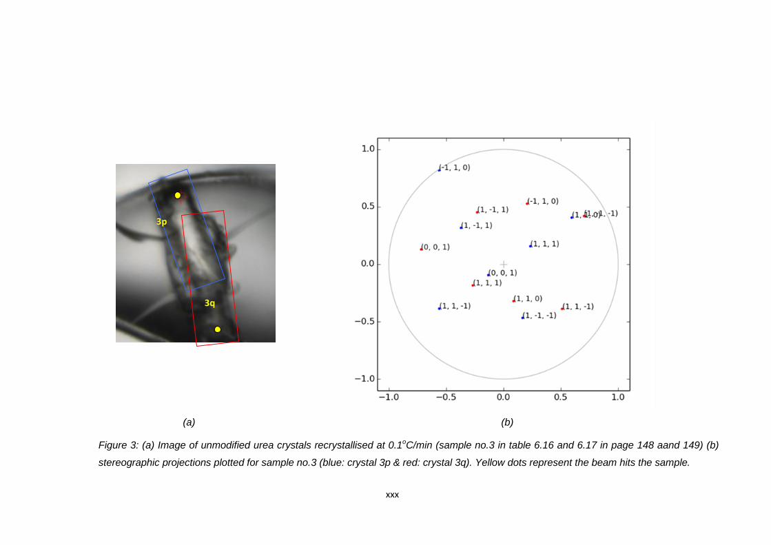
xxx

(a) (b)

Figure 3: (a) Image of unmodified urea crystals recrystallised at 0.1oC/min (sample no.3 in table 6.16 and 6.17 in page 148 aand 149) (b)


3p

3q

xxxi

(a) (b)

Figure 4: (a) Image of unmodified urea crystals recrystallised at 0.1oC/min (sample no.4 in table 6.16 and 6.17 in page 148 and 149), (b)


4p 4q

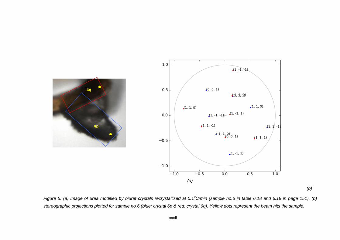
xxxii

(a)

(b)

Figure 5: (a) Image of urea modified by biuret crystals recrystallised at 0.10C/min (sample no.6 in table 6.18 and 6.19 in page 151), (b)


4p

4q

xxxiii

(a) (b)

Figure 6: (a) Image of urea modified by biuret crystals (0.1degC/min) (sample no.7 in Table 6.18 and 6.19 in paege 151), (b) stereographic

projections plotted for sample no.7 (blue: crystal 7p & red: crystal 7q). Yellow dots represent the beam hits the sample.

7p

7q

xxxiv

(a) (b)

Figure 7: (a) Image of urea modified by biuret crystals recrystallised at 0.1oC/min (sample no.9 in table 6.16 and 6.17 in page 151) (b)


8p

8q

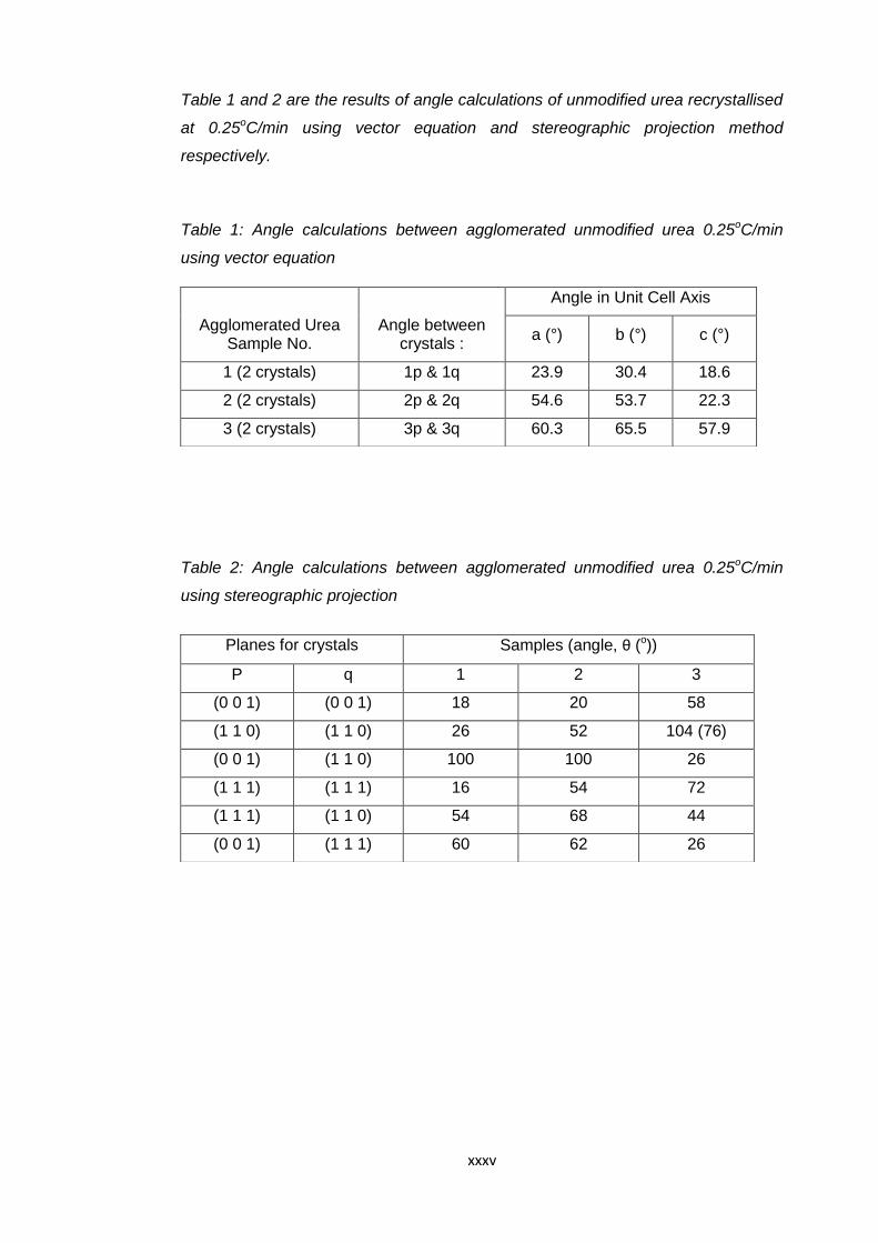
xxxv

Table 1 and 2 are the results of angle calculations of unmodified urea recrystallised

at 0.25oC/min using vector equation and stereographic projection method

respectively.

Table 1: Angle calculations between agglomerated unmodified urea 0.25oC/min




Agglomerated Urea Sample No.



a (°) b (°) c (°)

1 (2 crystals) 1p & 1q 23.9 30.4 18.6

2 (2 crystals) 2p & 2q 54.6 53.7 22.3

3 (2 crystals) 3p & 3q 60.3 65.5 57.9


P q 1 2 3

(0 0 1) (0 0 1) 18 20 58

(1 1 0) (1 1 0) 26 52 104 (76)

(0 0 1) (1 1 0) 100 100 26

(1 1 1) (1 1 1) 16 54 72

(1 1 1) (1 1 0) 54 68 44

(0 0 1) (1 1 1) 60 62 26

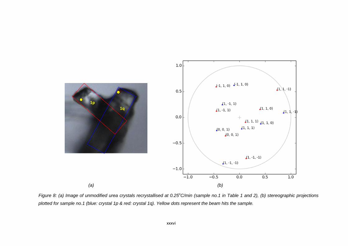
xxxvi

(a) (b)

Figure 8: (a) Image of unmodified urea crystals recrystallised at 0.25oC/min (sample no.1 in Table 1 and 2), (b) stereographic projections

plotted for sample no.1 (blue: crystal 1p & red: crystal 1q). Yellow dots represent the beam hits the sample.

1q

1p

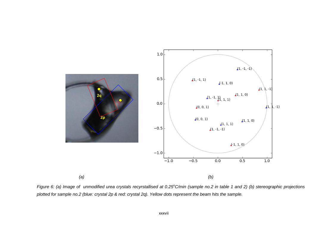
xxxvii

(a) (b)

Figure 6: (a) Image of unmodified urea crystals recyrstallised at 0.25oC/min (sample no.2 in table 1 and 2) (b) stereographic projections


2p

2q

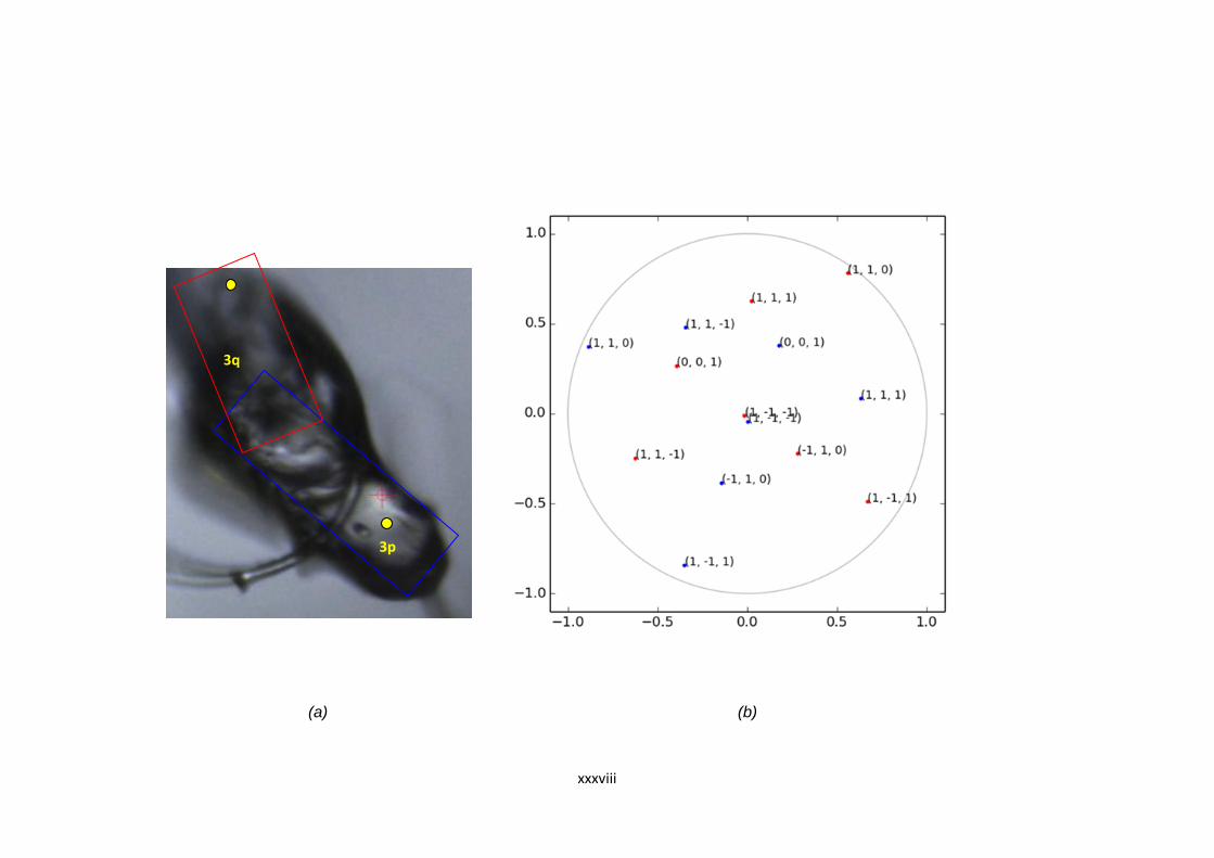
xxxviii

(a) (b)

3p

3q

xxxix

Figure 7: (a) Image of unmodified urea crystals recrystallised at 0.25oC/min (sample no.3 in table 1 and 2), (b) stereographic projections


xxxii

Table 3: Angle calculations between agglomerated urea modified by biuret

0.25oC/min using vector equation






a (°)

b (°)

c (°)

1 (2 crystals) 1p & 1q 17.5 28.3 31.7

2 (2 crystals) 2p & 2q 18.2 48.7 52.1


p q 1 2

(0 0 1) (0 0 1) 52 92

(1 1 0) (1 1 0) 133 (47) 72

(0 0 1) (1 1 0) 45 34

(1 1 1) (1 1 1) 32 80

(1 1 1) (1 1 0) 10 40

(0 0 1) (1 1 1) 80 52

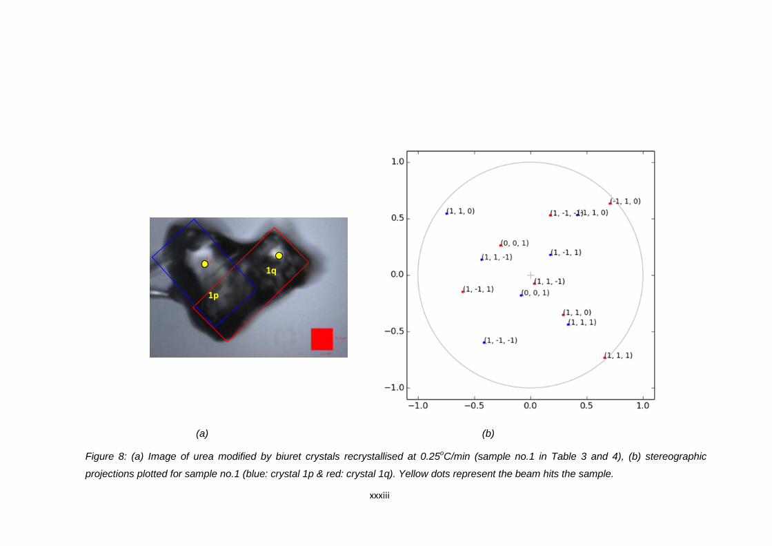
xxxiii

(a) (b)

Figure 8: (a) Image of urea modified by biuret crystals recrystallised at 0.25oC/min (sample no.1 in Table 3 and 4), (b) stereographic


1p

1q

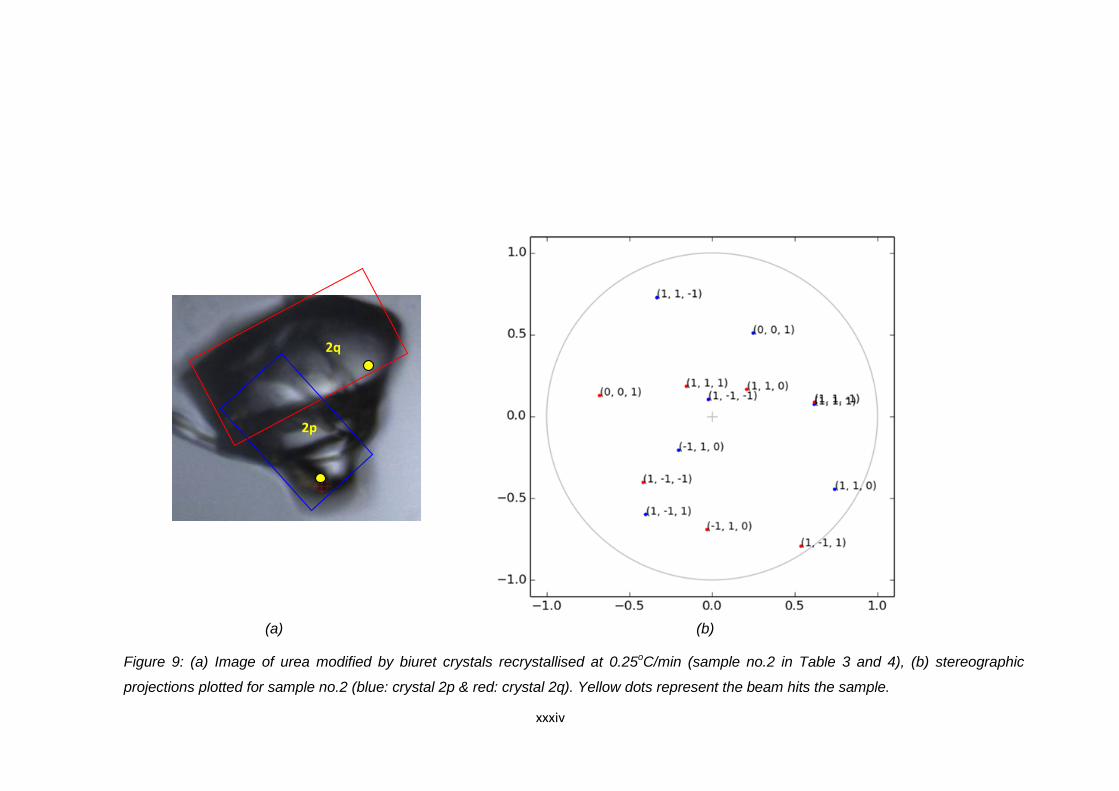
xxxiv

(a) (b)

Figure 9: (a) Image of urea modified by biuret crystals recrystallised at 0.25oC/min (sample no.2 in Table 3 and 4), (b) stereographic


2q

2p

xxxv

(a) (b)

Figure 10: (a) Image of unmodified urea crystals recrystallised at 0.5oC/min (sample no.10 in Table 6.20 and 6.21 in page 153). Blue and red

boxes indicate the position of the agglomerated crystals. The yellow spots indicate the point where the beam hits the crystal during data collection,

(b) stereographic projections plotted for sample no.10 (blue: crystal 10p & red: crystal 10q).

10p

10q

xxxvi






a (°) b (°) c (°)

1 (2 crystals) 1p & 1q 75.4 114.8 85.7

2 (2 crystals) 2p & 2q 63.4 68.5 68.7




p q 1 2

(0 0 1) (0 0 1) 90 68

(1 1 0) (1 1 0) 62 95

(0 0 1) (1 1 0) 40 34

(1 1 1) (1 1 1) 66 25

(1 1 1) (1 1 0) 34 64

(0 0 1) (1 1 1) 50 30

xxxvii

(a) (b)

Figure 11: Stereographic projection plotted for samples in Table 5 and 6 (blue: crystal p & red: crystal q) (a) sample no.1 (b)

sample no.2

xxxviii



Agglomerated Urea Sample No.



a (°) b (°) c (°)

1 (2 crystals) 1p & 1q 89.9 57.5 63.4

2 (2 crystals) 2p & 2q 12.1 73.1 74.1




p q 1 2

(0 0 1) (0 0 1) 64 76

(1 1 0) (1 1 0) 70 42

(0 0 1) (1 1 0) 86 58

(1 1 1) (1 1 1) 90 126

(1 1 1) (1 1 0) 72 104

(0 0 1) (1 1 1) 70 76

xxxix

(a) (b)

Figure 12: Stereographic projection plotted for samples in Table 7 and 8 (blue: crystal p & red: crystal q) (a) sample no.1 (b) sample

no.2

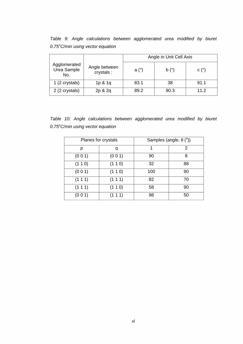
xl




No.



a (°) b (°) c (°)

1 (2 crystals) 1p & 1q 83.1 38 91.1

2 (2 crystals) 2p & 2q 89.2 90.3 11.2




p q 1 2

(0 0 1) (0 0 1) 90 8

(1 1 0) (1 1 0) 32 88

(0 0 1) (1 1 0) 100 90

(1 1 1) (1 1 1) 82 70

(1 1 1) (1 1 0) 58 90

(0 0 1) (1 1 1) 98 50

xli

(a) (b

Figure 13: Stereographic projection plotted for samples in Table 9 and 10 (blue: crystal p & red: crystal q) (a) sample no.1 (b) sample

no.2

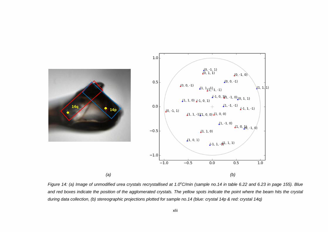
xlii

(a) (b)

Figure 14: (a) Image of unmodified urea crystals recrystallised at 1.0oC/min (sample no.14 in table 6.22 and 6.23 in page 155). Blue

and red boxes indicate the position of the agglomerated crystals. The yellow spots indicate the point where the beam hits the crystal

during data collection, (b) stereographic projections plotted for sample no.14 (blue: crystal 14p & red: crystal 14q)

14p 14q

xliii

(a) (b)

Figure 15: (a) Image of urea modified by biuret crystals recrystallised at 1.0oC/min (sample no.16 in Table 6.22 and 6.23 in page 155).

Blue and red boxes indicate the position of the agglomerated crystals. The yellow spots indicate the point where the beam hits the

crystal during data collection, (b) stereographic projections plotted for sample no.16 (blue: crystal 16p & red: crystal 16q).

16p

16q

Characterisation of the Morphological and Surface...

Documents

Transcript of Characterisation of the Morphological and Surface...