Character Recognition using Artificial Neural...

THE UNIVERSITY OF MANCHESTER

School of Computer Science

Character Recognition Using Artificial Neural Networks

Author: Farman Farmanov BSc (Hons) in Computer Science

Third Year Report 2014

Supervisor: Dr. Richard Neville

April 2014

1

Table of Contents The University Of Manchester ............................................................................................................................... 0

Abstract ................................................................................................................................................................. 4

Aknowledgement .................................................................................................................................................. 5

I. Introduction .................................................................................................................................................... 6

A. Project Aims .............................................................................................................................................. 6

B. Report Structure......................................................................................................................................... 6

II. Background ............................................................................................................................................... 7

A. Chapter Overview ...................................................................................................................................... 7

B. Introduction to Machine Learning ............................................................................................................. 7

C. Introduction to Character Recognition ...................................................................................................... 7

1) History of Optical Character Recognition ............................................................................................. 7

2) Character Recognition Process .............................................................................................................. 7

D. Introduction to Neural Networks ............................................................................................................... 8

1) Biological Inspiration ............................................................................................................................ 8

2) Artificial Neural Networks .................................................................................................................... 8

E. Learning Paradigms of Artificial Neural Networks ................................................................................... 9

1) Supervised Learning.............................................................................................................................. 9

2) Unsupervised Learning ......................................................................................................................... 9

F. Concluding Remarks ............................................................................................................................... 10

III. RESEARCH ............................................................................................................................................ 11

A. Chapter Overview .................................................................................................................................... 11

B. Supervised Learning Algorithms ............................................................................................................. 11

1) Perceptron ........................................................................................................................................... 11

2) Delta Rule ........................................................................................................................................... 12

3) Backpropagation ................................................................................................................................. 13

C. Software Development Methodology ...................................................................................................... 15

1) Waterfall Model .................................................................................................................................. 15

2) Agile Model ........................................................................................................................................ 15

3) Chosen methodology ........................................................................................................................... 16

D. Closing Remarks ..................................................................................................................................... 16

IV. Requirements ........................................................................................................................................... 17


B. Introduction to Requirements Engineering .............................................................................................. 17

C. Stakeholder Analysis ............................................................................................................................... 17

D. System Context Diagram ......................................................................................................................... 18

E. Use Cases ................................................................................................................................................ 18

F. Functional and Non-Functional requirements ......................................................................................... 19

G. Closing Remarks ..................................................................................................................................... 20

V. Design ...................................................................................................................................................... 21


B. Introduction ............................................................................................................................................. 21

2

C. Design Principles and Concepts .............................................................................................................. 21

D. Hierarchical Task Analysis ...................................................................................................................... 22

E. Class-Responsibility-Collaborator Cards ................................................................................................ 22

F. System Class Diagrams ........................................................................................................................... 23

G. Closing Remarks ..................................................................................................................................... 23

VI. Implementation ........................................................................................................................................ 24

A. Chapter Overview and Introduction ........................................................................................................ 24

B. Implementation Tools .............................................................................................................................. 24

1) Programming Language ...................................................................................................................... 24

2) Development Environment ................................................................................................................. 24

C. Prototyping .............................................................................................................................................. 24

1) Rapid Prototypes ................................................................................................................................. 25

2) Evolutionary Prototypes ...................................................................................................................... 25

D. Algorithmics and Data Structure ............................................................................................................. 26

1) Data Structure ..................................................................................................................................... 26

2) Algorithmics........................................................................................................................................ 26

E. Walkthrough ............................................................................................................................................ 27

F. Concluding Remarks ............................................................................................................................... 27

VII. Results ..................................................................................................................................................... 28


B. Final Results ............................................................................................................................................ 28

C. Parameter Analysis of the Backpropagation algorithm ........................................................................... 28

1) Learning Rate and Momentum ............................................................................................................ 29

2) Constructing Topology ........................................................................................................................ 30

D. Closing Remarks ..................................................................................................................................... 30

VIII. Testing ..................................................................................................................................................... 31


B. Introduction to Software Testing ............................................................................................................. 31

1) Black Box Testing ............................................................................................................................... 31

2) White Box Testing .............................................................................................................................. 31

IX. Evaluation and Conclusion ...................................................................................................................... 32

A. Chapter Overview and Introduction ........................................................................................................ 32

B. Project Evaluation ................................................................................................................................... 32

C. Further Improvements ............................................................................................................................. 32

D. Concluding Remarks ............................................................................................................................... 32

X. BIBLIOGRAPHY ................................................................................................................................... 33

XI. Appendix A ............................................................................................................................................. 36

XII. Appendix B .............................................................................................................................................. 37

XIII. Appendix C .............................................................................................................................................. 41

XIV. Appendix D ............................................................................................................................................. 42

Figure 1. Character Recognition Process ............................................................................................................... 6

3

Figure 2. Biological Neuron .................................................................................................................................. 8 Figure 3. Artificial neuron ..................................................................................................................................... 8 Figure 4. Single layered artificial neural network.................................................................................................. 9 Figure 5. Multilayered artificial neural network. ................................................................................................... 9 Figure 6. Pseudo code of perceptron learning rule .............................................................................................. 12 Figure 7. Error modulus graph. ............................................................................................................................ 12 Figure 8. Pseudo code of Backpropagation learning algorithm. .......................................................................... 13 Figure 9. Waterfall model life-cycle. This picture illustrates sequential behavior of waterfall model ................ 15 Figure 10. Development life-cycle of scrum ....................................................................................................... 16 Figure 11. Context Diagram. ................................................................................................................................ 18 Figure 12. Hand drawn Use Case Diagram. ........................................................................................................ 19 Figure 13. Hierarchical Task Analysis of the project ........................................................................................... 22 Figure 14. Hand drawn CRC cards ....................................................................................................................... 23 Figure 15. System System Class Diagram of Backpropagation algorithm .......................................................... 23 Figure 16. Prototypes developed during implementation of the project. ............................................................. 25 Figure 17. Hihh level pseudo code of backpropagation algorithm implemented in the final system ................... 27 Figure 18. Classification Rate. .............................................................................................................................. 28 Figure 19. 3-D graph of sensitivity analysis on learning rate and momentum .................................................... 29 Figure 20. Training process of a network with small and big learning rate .......................................................... 30 Figure 21. System Class Diagram of core character recognition system .............................................................. 36 Figure 22. Setting up neural network .................................................................................................................... 37 Figure 23. Identifying structure of neural network ............................................................................................... 37 Figure 24. Loading already trained network ......................................................................................................... 38 Figure 25. Indentifying training parameters ......................................................................................................... 38 Figure 26. Loading training data for the training .................................................................................................. 39 Figure 27. Starting the training ............................................................................................................................. 39 Figure 28. Viewing trainng graph ......................................................................................................................... 40 Figure 29. Test generalisablity ............................................................................................................................. 40 Figure 30. Sensitivity analysis of momentum and learning rate parameters ........................................................ 41 Figure 31. Sensitivity analysis of momentum rate and number of hidden units ................................................... 42

4

ABSTRACT

“We may hope that machines will eventually compete with men in all purely intellectual fields” Alan Turing

Is it possible to teach a machine to recognise characters, like human beings do? Artificial Neural Network is a

mathematic model, which is inspired from brain network structure of a human; it can be trained to recognise

patterns.

This paper covers research of an artificial neural networks and its utilization for character recognition purpose.

Software for recognition of handwritten character is developed throughout the project. Software engineering

approaches for gathering requirements, designing the system and testing were discussed explicitly throughout

the thesis. Final software, which successfully implemented the entire functional requirement, can be used to

investigate behavior of neural networks. Sensitivity analysis were undertaken in order to understand relationship

between training parameters. Project was successfully completed, as recognition rate of 90% were achieved.

5

AKNOWLEDGEMENT

I would like to thank my supervisor Dr. Richard Neville for his continues support and mentoring me during my

final year. Also, I want to thanks my friends and family, who were always supporting me.

6

I. INTRODUCTION

A. Project Aims

The aim of this project is to research artificial neural networks and training algorithms, and build complex

system that can recognise unknown handwritten characters. The software should have user friendly graphical

user interface that will allow user to upload training set. Neural network should train on given set of samples

and later recognise unknown handwritten character, which can be provided by user. Figure 1 illustrates process

of character recognition. Handwritten character is digitised and sent to a trained neural network; and network

will classify received character. This paper will cover development life-cycle of this project including research,

requirement gathering, system designing, implementation, testing and evaluation of results.

Figure 1. Character Recognition Process

B. Report Structure

This report is written according to IEEE standard for conference papers. The report consists of 7 main chapters:

i. Introduction chapter - gives a short description of problem domain.

ii. Background chapter - presents broad field of machine learning and character recognition,

followed by fundamental knowledge about neural networks.

iii. Research chapter - covers research done in subdomains of this project. The chapter

discusses supervised learning algorithms and software development methodologies.

iv. Requirements chapter - describes requirement gathering phase of this project. Presents functional

and non-functional table of requirements.

v. Design chapter - covers undertaken designing process of a system and provides artifacts

that are used during implementation phase.

vi. Implementation chapter – covers implementation phase of the project. Tools used for

development, and algorithms used to train a network are described in this chapter.

vii. Results chapter - presents analysis of the final system throughout experimental data.

viii. Testing chapter - covers testing methods of final system.

ix. Conclusion chapter - evaluates completed project, highlights areas for improvement and

concludes the report.

7

II. BACKGROUND

A. Chapter Overview

This chapter outlines background information needed before commencing to research stage. The chapter starts

with a brief introduction to Machine Learning. Moreover, character recognition process is described; and

fundamental information about artificial neural network is given. The chapter is concluded with the introduction

of various learning paradigms of artificial neural networks.

B. Introduction to Machine Learning

Machine Learning is a branch of Artificial Intelligence that studies how systems can be taught to learn from

previous experience [1]. The produced system has an ability to adapt to changes in environment and

approximate results according to gathered data without human intervention. Nowadays, applications of machine

learning can be seen in many fields like retailing, finance, business and science. Spam-filter, face detection,

weather prediction, medical diagnosis and optical character recognition are examples of problems that can be

solved using machine learning [2]. Further sub-chapters will cover character recognition process in details.

C. Introduction to Character Recognition

Optical Character Recognition (OCR) is a process of converting scanned image of handwritten characters into

machine readable text [3]. OCR is considered a subfield of pattern recognition where system assigns input to

one of the given classes. Numbers, characters and notations are presented to an OCR machine which classifies

unknown input by comparing it to introduced examples. This next section considers the OCR process and its

history.

1) History of Optical Character Recognition

Origins of OCR can be traced to the early 20th

century. One of the first OCR machines was developed by

Emanuel Goldberg in 1914 [4]. Goldberg’s machine was reading characters and transferring them into telegraph

code. During that period Edmund Fournier d’Albe build a machine called Otophone, whose purpose was aiding

blind people by producing tones when devices were moved over letters [5].

During the 1950s, Intelligent Machines Research Corporation (IMRC) produced the first commercially used

OCR machines that were sold to Reader’s Digest, Standard Oil Company, Ohio Bell Telephone Company for

reading reports and bills [6]. These OCR machines were cost-effective way to handle data entry. In the mid-

1960s a new generation of OCR machines were introduced which could recognise handwritten digits and some

characters [6]. As years passed character recognition rate of new OCR machines were increased. Today OCRs

are widely used as their recognition rate of typewritten text is over 90%. However, the perfect rate can be

obtained after human inspection [6]. Handwriting recognition and text written in other languages are still

considered subjects of research.

2) Character Recognition Process

Character Recognition process can be broken down into 3 main stages; Pre-processing, Feature Extraction and

Artificial Neural Network (ANN) modeling. Pre-processing is considered as a first phase of character recognition

process and to increase chance of recognition, the image is improved. Noise, tilted image, distortion and other

factors that can affect recognition rate can be removed by pre-processing. The following pre-processing methods

are commonly used in character recognition software [7]:

i. Binarisation - Image is converted into binary (black-and-white) scale for decreasing

computational power of learning algorithm. Threshold pixel value is chosen. Pixels below that

value assumed as white regions when higher pixels assigned to be black.

ii. Thinning - Using edge detection algorithm, character’s width is thinned to 1 pixel. This

helps to make characters uniform and reduce redundancy.

iii. Normalisation - Position, aptitude and size of a character is normalized according to chosen

template.

8

Later, pre-processed image is transformed into dimensionally reduced representation. Simplifying large data

decreases computation time of recognition process. Reduced representation is called “features”, and process of

choosing feature referred to as “feature extraction” [7]. Finally, extracted features are passed to artificial neural

network where training and simulation happens. This project concentrates on investigating and applying

artificial neural network. Next section introduces basic concepts of artificial neural network.

D. Introduction to Neural Networks

1) Biological Inspiration

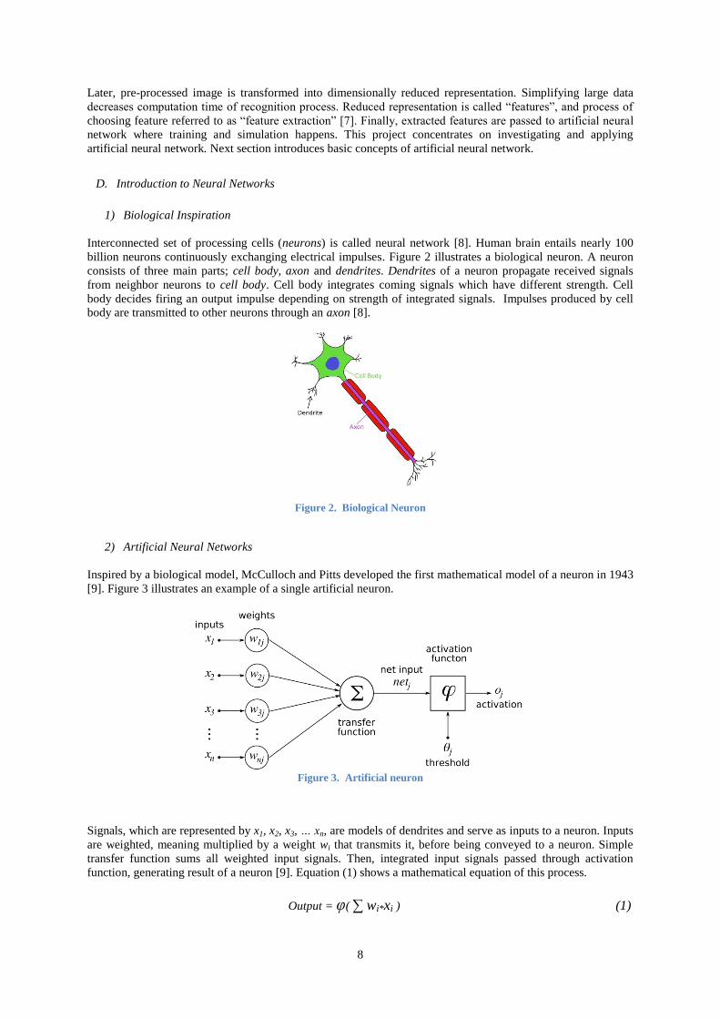
Interconnected set of processing cells (neurons) is called neural network [8]. Human brain entails nearly 100

billion neurons continuously exchanging electrical impulses. Figure 2 illustrates a biological neuron. A neuron

consists of three main parts; cell body, axon and dendrites. Dendrites of a neuron propagate received signals

from neighbor neurons to cell body. Cell body integrates coming signals which have different strength. Cell

body decides firing an output impulse depending on strength of integrated signals. Impulses produced by cell

body are transmitted to other neurons through an axon [8].

Figure 2. Biological Neuron

2) Artificial Neural Networks

Inspired by a biological model, McCulloch and Pitts developed the first mathematical model of a neuron in 1943

[9]. Figure 3 illustrates an example of a single artificial neuron.

Figure 3. Artificial neuron

Signals, which are represented by x1, x2, x3, … xn, are models of dendrites and serve as inputs to a neuron. Inputs

are weighted, meaning multiplied by a weight wi that transmits it, before being conveyed to a neuron. Simple

transfer function sums all weighted input signals. Then, integrated input signals passed through activation

function, generating result of a neuron [9]. Equation (1) shows a mathematical equation of this process.

Output = φ( ∑ wi*xi ) (1)

9

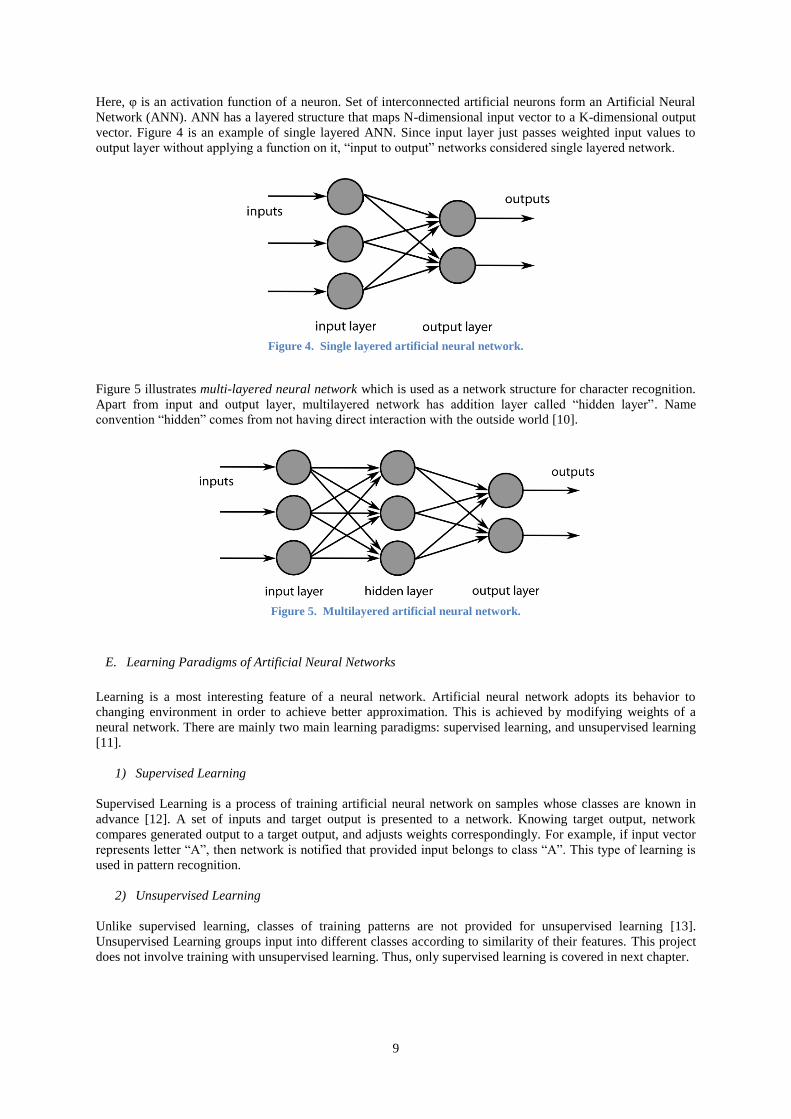
Here, φ is an activation function of a neuron. Set of interconnected artificial neurons form an Artificial Neural

Network (ANN). ANN has a layered structure that maps N-dimensional input vector to a K-dimensional output

vector. Figure 4 is an example of single layered ANN. Since input layer just passes weighted input values to

output layer without applying a function on it, “input to output” networks considered single layered network.

Figure 4. Single layered artificial neural network.

Figure 5 illustrates multi-layered neural network which is used as a network structure for character recognition.

Apart from input and output layer, multilayered network has addition layer called “hidden layer”. Name

convention “hidden” comes from not having direct interaction with the outside world [10].

Figure 5. Multilayered artificial neural network.

E. Learning Paradigms of Artificial Neural Networks

Learning is a most interesting feature of a neural network. Artificial neural network adopts its behavior to

changing environment in order to achieve better approximation. This is achieved by modifying weights of a

neural network. There are mainly two main learning paradigms: supervised learning, and unsupervised learning

[11].

1) Supervised Learning

Supervised Learning is a process of training artificial neural network on samples whose classes are known in

advance [12]. A set of inputs and target output is presented to a network. Knowing target output, network

compares generated output to a target output, and adjusts weights correspondingly. For example, if input vector

represents letter “A”, then network is notified that provided input belongs to class “A”. This type of learning is

used in pattern recognition.

2) Unsupervised Learning

Unlike supervised learning, classes of training patterns are not provided for unsupervised learning [13].

Unsupervised Learning groups input into different classes according to similarity of their features. This project

does not involve training with unsupervised learning. Thus, only supervised learning is covered in next chapter.

10

F. Concluding Remarks

This chapter introduced character recognition process and fundamental information about artificial neural

network. The next chapter looks into undertaken research about supervised learning algorithms and software

development methodologies.

11

III. RESEARCH

A. Chapter Overview

This chapter covers research undertaken in subdomains of character recognition project. The first research

domain, software development methodology, encapsulates various methodologies and practices considered for

development of the project. Supervised learning research domain looks into theory behind different supervised

learning algorithms.

B. Supervised Learning Algorithms

Supervised learning is one of the well-known learning paradigms in machine learning. Neural network is trained

by examples where desired output is presented [11]. Therefore, weights of a neural network adopted in respect

to previous classification error. As discussed in background chapter architecture of a neural network depends on

number and type of classes to be recognised. Single layered network can be sufficient for linearly separable

classes, when for non-linear case multi-layered neural network is applied. Adjustments of weights in neural

network are conducted by learning algorithms. Learning algorithms are also referred to as training rules or

training algorithms. This section discusses various learning algorithms that were researched during this project.

1) Perceptron

Perceptron is a linear classifier for binary classes that uses single-layered network. This algorithm was

suggested by Frank Rosenblatt in 1957 for solving linearly separable classification problems [15]. Classification

of an input sample is evaluated by simple threshold logic where activation of a network compared to a threshold

value. Activation of a perceptron is a produced by dot product of input (x) and weight (w) vectors of a neural

network. If the activation value is greater than the threshold, then the output of a network is “1” and “0” if it is

less [15]. An equation of simple threshold logic unit (TLU), which is applied in perceptron, is

(2)

where w represents weights of a neuron and ɵ denotes a threshold value. If N-dimensional input samples of two

different classes are linearly separable then there exist a hyperplane that isolates these classes [15]. In neural

networks this hyperplane is referred to as a decision surface and its equation is

w1*x1 + w2*x2 + ….. + wn*xn - ɵ = 0 (3)

Because inputs (x) are constant, weights and threshold are modified in order to get desired decision surface.

This process is called training of the neural network [15]. Input samples which referred to as a training set is

provided to perceptron algorithm for training. Small modification to weights and threshold is made in case result

produced by perceptron is different than target output of supervised training sample. For simplicity, threshold

value is treated as weights by moving it to the left of equation 1 and to be accounted as (n+1)st dimension when

value of xn+1 will be “-1”. Adjustment of weights for each sample is done by equation

wi = wi + α*(t - y)*xi (4)

where t signifies target output and y is a result of neural network which is evaluated by equation 1. Most

important parameter of learning algorithms is learning rate which is denoted by α. Learning rate affects amount

of change made to weights [16]. When target (t) is equal to actual output (y) then changes in weights are not

affected since difference between t and y is 0.

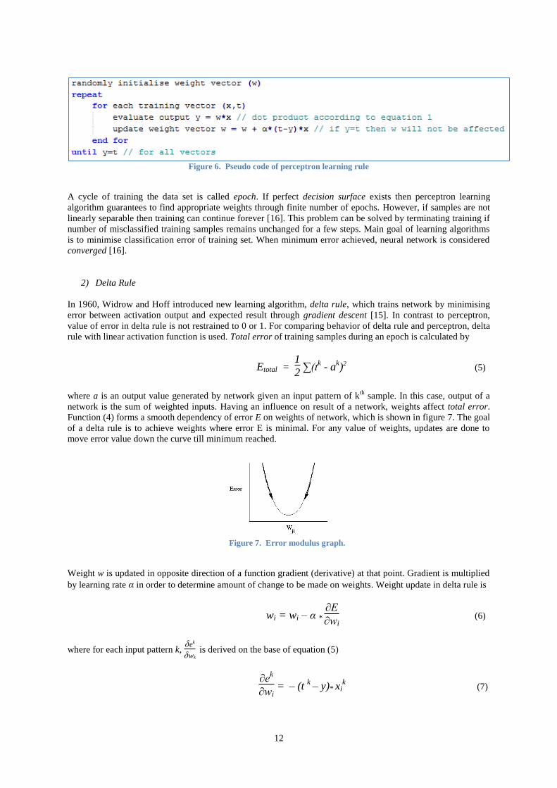
Training in perceptron algorithm continues until results of all training samples match target values. Figure 6

illustrates pseudocode of perceptron learning algorithm.

12

Figure 6. Pseudo code of perceptron learning rule

A cycle of training the data set is called epoch. If perfect decision surface exists then perceptron learning

algorithm guarantees to find appropriate weights through finite number of epochs. However, if samples are not

linearly separable then training can continue forever [16]. This problem can be solved by terminating training if

number of misclassified training samples remains unchanged for a few steps. Main goal of learning algorithms

is to minimise classification error of training set. When minimum error achieved, neural network is considered

converged [16].

2) Delta Rule

In 1960, Widrow and Hoff introduced new learning algorithm, delta rule, which trains network by minimising

error between activation output and expected result through gradient descent [15]. In contrast to perceptron,

value of error in delta rule is not restrained to 0 or 1. For comparing behavior of delta rule and perceptron, delta

rule with linear activation function is used. Total error of training samples during an epoch is calculated by

Etotal = 1

2 ∑(t

k - a

k)2

(5)

where a is an output value generated by network given an input pattern of kth

sample. In this case, output of a

network is the sum of weighted inputs. Having an influence on result of a network, weights affect total error.

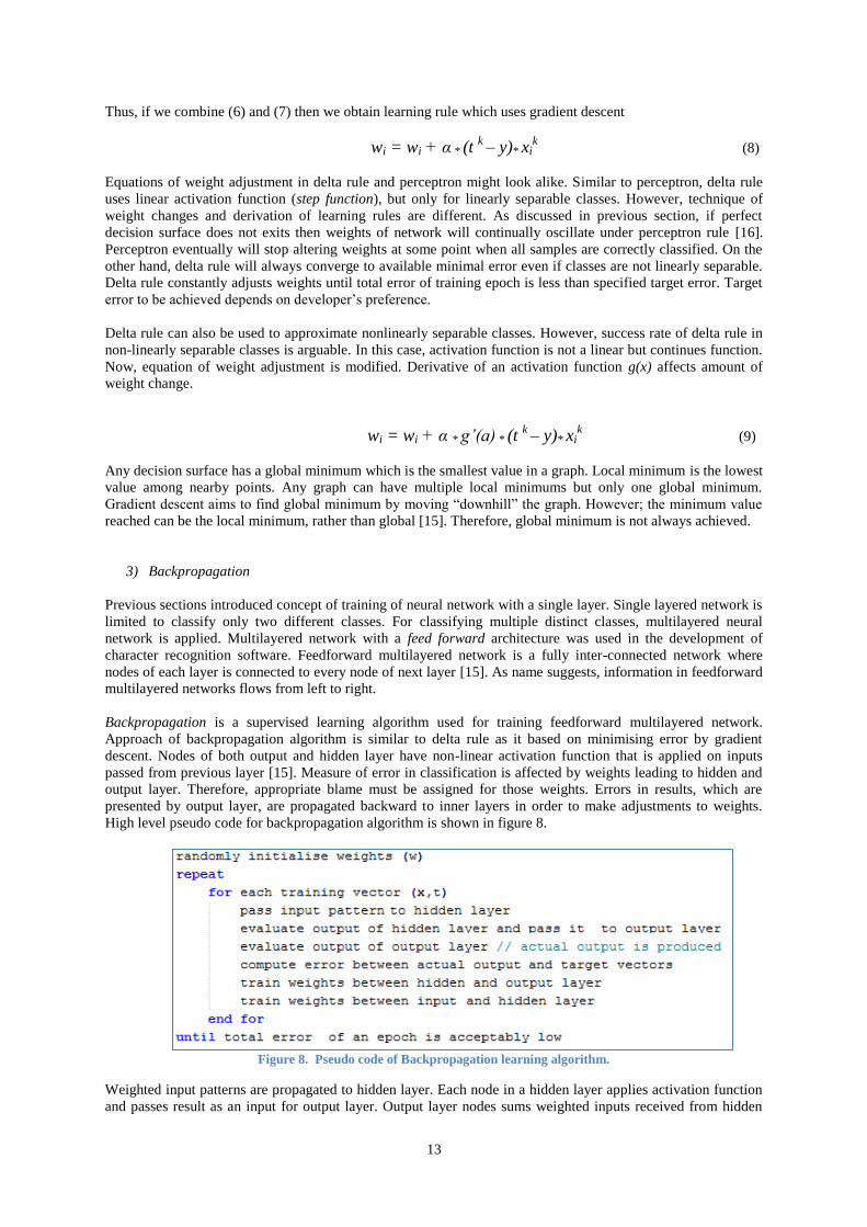
Function (4) forms a smooth dependency of error E on weights of network, which is shown in figure 7. The goal

of a delta rule is to achieve weights where error E is minimal. For any value of weights, updates are done to

move error value down the curve till minimum reached.

Figure 7. Error modulus graph.

Weight w is updated in opposite direction of a function gradient (derivative) at that point. Gradient is multiplied

by learning rate α in order to determine amount of change to be made on weights. Weight update in delta rule is

wi = wi – α *

∂E

∂wi (6)

where for each input pattern k, δek

δwk

is derived on the base of equation (5)

∂ek

∂wi =

– (t

k – y)* xi

k (7)

13

Thus, if we combine (6) and (7) then we obtain learning rule which uses gradient descent

wi = wi + α * (t k – y)* xi

k (8)

Equations of weight adjustment in delta rule and perceptron might look alike. Similar to perceptron, delta rule

uses linear activation function (step function), but only for linearly separable classes. However, technique of

weight changes and derivation of learning rules are different. As discussed in previous section, if perfect

decision surface does not exits then weights of network will continually oscillate under perceptron rule [16].

Perceptron eventually will stop altering weights at some point when all samples are correctly classified. On the

other hand, delta rule will always converge to available minimal error even if classes are not linearly separable.

Delta rule constantly adjusts weights until total error of training epoch is less than specified target error. Target

error to be achieved depends on developer’s preference.

Delta rule can also be used to approximate nonlinearly separable classes. However, success rate of delta rule in

non-linearly separable classes is arguable. In this case, activation function is not a linear but continues function.

Now, equation of weight adjustment is modified. Derivative of an activation function g(x) affects amount of

weight change.

wi = wi + α * g’(a) * (t k – y)* xi

k (9)

Any decision surface has a global minimum which is the smallest value in a graph. Local minimum is the lowest

value among nearby points. Any graph can have multiple local minimums but only one global minimum.

Gradient descent aims to find global minimum by moving “downhill” the graph. However; the minimum value

reached can be the local minimum, rather than global [15]. Therefore, global minimum is not always achieved.

3) Backpropagation

Previous sections introduced concept of training of neural network with a single layer. Single layered network is

limited to classify only two different classes. For classifying multiple distinct classes, multilayered neural

network is applied. Multilayered network with a feed forward architecture was used in the development of

character recognition software. Feedforward multilayered network is a fully inter-connected network where

nodes of each layer is connected to every node of next layer [15]. As name suggests, information in feedforward

multilayered networks flows from left to right.

Backpropagation is a supervised learning algorithm used for training feedforward multilayered network.

Approach of backpropagation algorithm is similar to delta rule as it based on minimising error by gradient

descent. Nodes of both output and hidden layer have non-linear activation function that is applied on inputs

passed from previous layer [15]. Measure of error in classification is affected by weights leading to hidden and

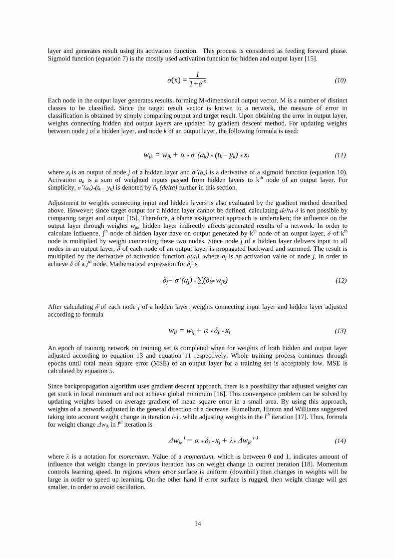
output layer. Therefore, appropriate blame must be assigned for those weights. Errors in results, which are

presented by output layer, are propagated backward to inner layers in order to make adjustments to weights.

High level pseudo code for backpropagation algorithm is shown in figure 8.

Figure 8. Pseudo code of Backpropagation learning algorithm.

Weighted input patterns are propagated to hidden layer. Each node in a hidden layer applies activation function

and passes result as an input for output layer. Output layer nodes sums weighted inputs received from hidden

14

layer and generates result using its activation function. This process is considered as feeding forward phase.

Sigmoid function (equation 7) is the mostly used activation function for hidden and output layer [15].

σ(x) = 1

1+e-x (10)

Each node in the output layer generates results, forming M-dimensional output vector. M is a number of distinct

classes to be classified. Since the target result vector is known to a network, the measure of error in

classification is obtained by simply comparing output and target result. Upon obtaining the error in output layer,

weights connecting hidden and output layers are updated by gradient descent method. For updating weights

between node j of a hidden layer, and node k of an output layer, the following formula is used:

wjk = wjk + α * σ’(ak) * (tk – yk) * xj (11)

where xj is an output of node j of a hidden layer and σ’(ak) is a derivative of a sigmoid function (equation 10).

Activation ak is a sum of weighted inputs passed from hidden layers to kth

node of an output layer. For

simplicity, σ’(ak)*(tk – yk) is denoted by δk (delta) further in this section.

Adjustment to weights connecting input and hidden layers is also evaluated by the gradient method described

above. However; since target output for a hidden layer cannot be defined, calculating delta δ is not possible by

comparing target and output [15]. Therefore, a blame assignment approach is undertaken; the influence on the

output layer through weights wjk, hidden layer indirectly affects generated results of a network. In order to

calculate influence, jth

node of hidden layer have on output generated by kth

node of an output layer, δ of kth

node is multiplied by weight connecting these two nodes. Since node j of a hidden layer delivers input to all

nodes in an output layer, δ of each node of an output layer is propagated backward and summed. The result is

multiplied by the derivative of activation function σ(aj), where aj is an activation value of node j, in order to

achieve δ of a jth

node. Mathematical expression for δj is

δj = σ’(aj) * ∑(δk* wjk) (12)

After calculating δ of each node j of a hidden layer, weights connecting input layer and hidden layer adjusted

according to formula

wij = wij + α * δj * xi (13)

An epoch of training network on training set is completed when for weights of both hidden and output layer

adjusted according to equation 13 and equation 11 respectively. Whole training process continues through

epochs until total mean square error (MSE) of an output layer for a training set is acceptably low. MSE is

calculated by equation 5.

Since backpropagation algorithm uses gradient descent approach, there is a possibility that adjusted weights can

get stuck in local minimum and not achieve global minimum [16]. This convergence problem can be solved by

updating weights based on average gradient of mean square error in a small area. By using this approach,

weights of a network adjusted in the general direction of a decrease. Rumelhart, Hinton and Williams suggested

taking into account weight change in iteration l-1, while adjusting weights in the lth

iteration [17]. Thus, formula

for weight change Δwjk in lth

iteration is

Δwjk l = α * δj * xj + λ* Δwjk

l-1 (14)

where λ is a notation for momentum. Value of a momentum, which is between 0 and 1, indicates amount of

influence that weight change in previous iteration has on weight change in current iteration [18]. Momentum

controls learning speed. In regions where error surface is uniform (downhill) then changes in weights will be

large in order to speed up learning. On the other hand if error surface is rugged, then weight change will get

smaller, in order to avoid oscillation.

15

C. Software Development Methodology

Software development methodology is a software engineering approach for planning, designing, implementation

and maintaining large-scaled software [19Rules and phases specified by chosen methodology are followed in

order to efficiently develop and deliver the final product. There are two main types of methodologies: sequential

and cyclical. Sequential methodology suggests approaching software development phases in sequence. Firstly

planning phase completed, then the designing phase proceeded by implementation phase and finalised by testing

phase. Waterfall is an example of sequential methodology. However, cyclical methodology proposes iterating

over phases. Small proportion of planning, designing, implementation and testing process evaluated for the each

iteration until final product is ready. Spiral model is considered a cyclic methodology [20]. Performance of

methodology differs depending on various aspects like deliverables, tools, environment and etc. Several

methodologies, analysis of which is given in the next section, were considered for development of this project.

1) Waterfall Model

Waterfall is a sequential methodology where each project phase commenced only if previous phase is finished.

Once completed, preceding phases never approached. All requirement and project plan must be clarified in

advance. Figure 9 illustrates life-cycle of a waterfall process. In theory, projects that use Waterfall method result

in fast deployment of working software [21]. However, this assumption proved to be incorrect in practice [22].

Requirements gathered at the beginning of the project are not guaranteed to be stable. Considering sequential

behavior of waterfall methodology, a significant amount of time passes from requirement phase until software is

deployed. Therefore, if a customer changes some requirements towards the end of the project completion, these

amendments will incur a reasonable amount of time and effort. Moreover, in waterfall method, software cannot

be tested until the implementation phase is completed [23].

Figure 9. Waterfall model life-cycle.

This picture illustrates sequential behavior of waterfall model

2) Agile Model

Agile software development is a set of methodologies that propose development by iterative and incremental

approach. Iteration involves following whole development cycle, at the end of which, working software is

produced. Software evolves gradually through multiple iterations. Agile manifesto for agile software

development suggests four core values that all agile methods agree on [24]:

1. Individuals and interactions over processes and tools.

2. Working software over comprehensive documentation.

3. Customer collaboration over contract negotiation.

4. Responding to change over following a plan.

Agile methodology stresses importance of constant interaction with customer and other team members. Since

development process proceeded through time-boxed iterations, working software frequently presented to

customer for reviewing. Requirements are never gather upfront in agile methodology, but identified only after

receiving customer feedback [25]. Therefore, any changes in requirement or design of software can be quickly

implemented. Also, at the commencement of the project unclear requirements can be clarified and implemented

in later iterations. As mentioned earlier, there are various methods of agile software that have common values

but different set of practices; XP and SCRUM are most well-known agile methods.

16

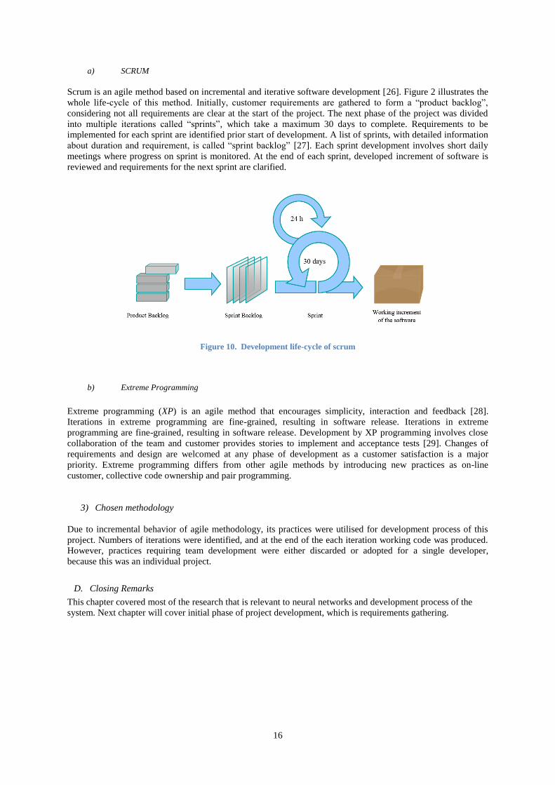
a) SCRUM

Scrum is an agile method based on incremental and iterative software development [26]. Figure 2 illustrates the

whole life-cycle of this method. Initially, customer requirements are gathered to form a “product backlog”,

considering not all requirements are clear at the start of the project. The next phase of the project was divided

into multiple iterations called “sprints”, which take a maximum 30 days to complete. Requirements to be

implemented for each sprint are identified prior start of development. A list of sprints, with detailed information

about duration and requirement, is called “sprint backlog” [27]. Each sprint development involves short daily

meetings where progress on sprint is monitored. At the end of each sprint, developed increment of software is

reviewed and requirements for the next sprint are clarified.

Figure 10. Development life-cycle of scrum

b) Extreme Programming

Extreme programming (XP) is an agile method that encourages simplicity, interaction and feedback [28].

Iterations in extreme programming are fine-grained, resulting in software release. Iterations in extreme

programming are fine-grained, resulting in software release. Development by XP programming involves close

collaboration of the team and customer provides stories to implement and acceptance tests [29]. Changes of

requirements and design are welcomed at any phase of development as a customer satisfaction is a major

priority. Extreme programming differs from other agile methods by introducing new practices as on-line

customer, collective code ownership and pair programming.

3) Chosen methodology

Due to incremental behavior of agile methodology, its practices were utilised for development process of this

project. Numbers of iterations were identified, and at the end of the each iteration working code was produced.

However, practices requiring team development were either discarded or adopted for a single developer,

because this was an individual project.

D. Closing Remarks

This chapter covered most of the research that is relevant to neural networks and development process of the

system. Next chapter will cover initial phase of project development, which is requirements gathering.

17

IV. REQUIREMENTS

A. Chapter Overview

This chapter covers the following phases of requirement engineering: requirement elicitation, analysis and

requirement documentation. The chapter also gives a detailed and informative introduction relating to the theory

of requirement engineering and the functions the system needs to provide; these are discussed and supported

with a set of descriptive functional and non-functional tables.

B. Introduction to Requirements Engineering

The requirements documentation describes how software should function [30]. Therefore establishing and

managing requirements is essential in software development. Requirements engineering process encapsulates

everything concerning requirements which is mainly gathering, documenting and managing requirement [39].

Requirement engineering consists of four phases: elicitation, negotiation, specification and validation. In

elicitation phase, stakeholders who will interact with a system are discovered and approached in order to clarify

requirements. Various techniques were used to obtain requirements from stakeholders. Personal interviews,

questionnaires, surveys, observation and demonstration of product prototypes or the product itself are the most

commonly used methods in practice [40]. Clarified requirements were documented in details using diagrams and

tables which will assist development process. Stakeholder table, context and use case diagram, functional and

nonfunctional requirements table illustrated further in this chapter are artefacts that will help in development of

character recognition project. Validating requirements is quite important as user satisfaction is a priority in

project development [37]. However, agile methodology suggests that change of requirement is inevitable during

projects. Most of documentation is useless since requirements documented are no longer implemented or

changed. Extreme programming recommends writing down user stories and clarifying each of them just before

implementing it [41]. Main principles of agile methodology applied in this project and only relevant

documentation of requirement done.

C. Stakeholder Analysis

A Stakeholder is a person or group who is afflicted by system or can have an impact on requirements [31].

Identifying stakeholders at the early stage of the project is crucial for establishing and clarifying requirements.

Interest-influence grid is a method of stakeholder mapping proposed by Imperial College London [42] in order

to grasp level of engagement with a particular stakeholder. This project can be considered small-scaled project

there is only limited number of stakeholders who have different level of influence on the system. Table 1

illustrates title of stakeholder, responsibility, interest and influence on this project. Influence column indicates

level of impact particular stakeholder has on development of project. Interest column shows interest of a

stakeholder in final product. It can be seen from the table, that there are mainly to types of stakeholders.

Stakeholders, having high interest and high influence level, should be interacted frequently in order to clarify

requirements and get a feedback. Low influence and high interest indicate that stakeholder should be informed

about changes in the project.

Table 1. Stakeholder Analysis

Stakeholder

Influence Interest Responsibility

Developer

High

High

Designing, implementing and testing the system.

Supervisor High High Supervising developer

through development of a

system.

Second Marker Low High Assessing and providing

feedback.

User Low High Using system to test

recognition functionality

18

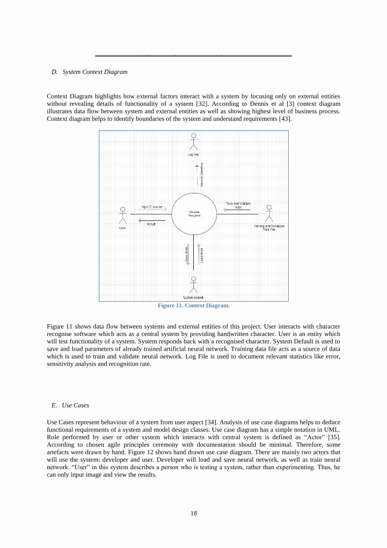
D. System Context Diagram

Context Diagram highlights how external factors interact with a system by focusing only on external entities

without revealing details of functionality of a system [32]. According to Dennis et al [3] context diagram

illustrates data flow between system and external entities as well as showing highest level of business process.

Context diagram helps to identify boundaries of the system and understand requirements [43].

Figure 11. Context Diagram.

Figure 11 shows data flow between systems and external entities of this project. User interacts with character

recognise software which acts as a central system by providing handwritten character. User is an entity which

will test functionality of a system. System responds back with a recognised character. System Default is used to

save and load parameters of already trained artificial neural network. Training data file acts as a source of data

which is used to train and validate neural network. Log File is used to document relevant statistics like error,

sensitivity analysis and recognition rate.

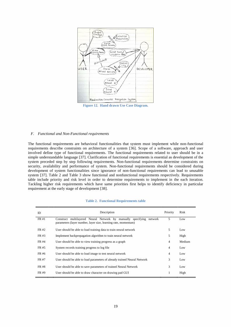
E. Use Cases

Use Cases represent behaviour of a system from user aspect [34]. Analysis of use case diagrams helps to deduce

functional requirements of a system and model design classes. Use case diagram has a simple notation in UML.

Role performed by user or other system which interacts with central system is defined as “Actor” [35].

According to chosen agile principles ceremony with documentation should be minimal. Therefore, some

artefacts were drawn by hand. Figure 12 shows hand drawn use case diagram. There are mainly two actors that

will use the system: developer and user. Developer will load and save neural network, as well as train neural

network. “User” in this system describes a person who is testing a system, rather than experimenting. Thus, he

can only input image and view the results.

19

Figure 12. Hand drawn Use Case Diagram.

F. Functional and Non-Functional requirements

The functional requirements are behavioral functionalities that system must implement while non-functional

requirements describe constraints on architecture of a system [36]. Scope of a software, approach and user

involved define type of functional requirements. The functional requirements related to user should be in a

simple understandable language [37]. Clarification of functional requirements is essential as development of the

system preceded step by step following requirements. Non-functional requirements determine constraints on

security, availability and performance of system. Non-functional requirements should be considered during

development of system functionalities since ignorance of non-functional requirements can lead to unusable

system [37]. Table 2 and Table 3 show functional and nonfunctional requirements respectively. Requirements

table include priority and risk level in order to determine requirements to implement in the each iteration.

Tackling higher risk requirements which have same priorities first helps to identify deficiency in particular

requirement at the early stage of development [38].

Table 2. Functional Requirements table

ID

Description Priority Risk

FR #1 Construct multilayered Neural Network by manually specifying network

parameters (layer number, layer size, learning rate, momentum)

5 Low

FR #2 User should be able to load training data to train neural network 5 Low

FR #3 Implement backpropagation algorithm to train neural network 5 High

FR #4 User should be able to view training progress as a graph 4 Medium

FR #5 System records training progress to log file 4 Low

FR #6 User should be able to load image to test neural network 4 Low

FR #7 User should be able to load parameters of already trained Neural Network

3 Low

FR #8 User should be able to save parameters of trained Neural Network 3 Low

FR #9 User should be able to draw character on drawing pad GUI 1 High

20

Table 3. Non-Functional Requirements table

ID

Description Priority Risk

NFR #1 GUI should be easy to use, just by following notations 5 Low

NFR #2 System should work on Windows, Linux and MacOS 3 Low

G. Closing Remarks

This chapter described step-by-step process of requirement discovery that will be considered in software

development. Next chapter focusses on design classes that define structure of a system.

21

V. DESIGN

A. Chapter Overview

This chapter describes the design process utilised for this character recognition project. In order to highlight the

theory applied, the chapter is supported by the theoretical diagrammatic design abstraction technique UML; and

hence UML diagrams and schemes are utilised throughout this chapter. The chapter starts by introducing design

principles and concepts. Architectural design of this project illustrated at various abstraction levels through this

chapter.

B. Introduction

The software design phase is an iterative process that is applied after analysing gathered requirements (Table 2

and Table 3) in order to translate requirements into a structured plan for software construction [44]. Also quality

of the software can be assessed before and during construction, thus revealing flaws of a system in early stages

of development. Suggested guidelines and technical criteria are followed throughout the design process in order

to achieve high design quality. The next section discusses main design principles and concepts applied in this

project [45].

C. Design Principles and Concepts

Design principles guide software engineer to construct high quality system design. Following principles applied

during design phase of this project

i. The design should be easily altered in order to respond to changes.

ii. Integrity and uniformity is crucial in good design.

iii. Design should be in higher abstraction level that coding logic.

Applied principles increase quality of a software design from both external and internal perspective. Software

properties like reliability, speed and usability that monitored by users are considered external quality factors.

Internal quality factors considered by software engineers and discovered through following basic design

concepts [45]:

i. Modularity - Complex problems are easier solved by divide and conquer method which is

splitting problem into smaller ones. Modularity concept suggests dividing system into small

modules which helps to manage system. However, large number of modules leads to more

effort spent on integrating modules.

ii. Information Hiding - Information within each module should be public only for modules

that actually need that information. Information hiding concept is very useful when it comes

to later amendments needed in the project. Thus errors occurred in a class will not affect

others.

iii. Abstraction - Modular solution to problems involve designing software at various levels of

abstraction. Continuous revisions and refinements of high-level design which encapsulates

overview of functionalities lead to design describing low-level details and algorithms to be

considered [2]. Further chapters outline design components used for character recognition

project by showing transition from high-level to lower level of abstraction.

22

D. Hierarchical Task Analysis

Hierarchical Task Analysis (HTA) is aligned to HCI and is a task analysis technique that is untilised after the

requirements analysis phase. HTA is a goal-oriented approach which describes hierarchical organisation of tasks

to be achieved within the context of main goal [46]. HTA is structured in a top-down manner where the top goal

is the main objective of software. Then, higher-level goals are fine-grained into sub-goals. This process

continues recursively until analyst is assured that further refinements are unnecessary. Finally, all the goals in

the hierarchy are implemented in order to achieve sublime goal. HTA also describes precondition and order in

which subgoals are attained [47]. Figure 13 illustrates an HTA graph of Character Recognition project. HTA is

later used as an error analysis and aid to system design. Main goal is to achieve character recognition. To do

that, 3 sub-goals must be achieved: setting up network, training network and testing network. Each of this task

are also divided into sub-goals.

Figure 13. Hierarchical Task Analysis of the project

E. Class-Responsibility-Collaborator Cards

The Class-Responsibility-Collaborator (CRC) Cards is an object-oriented analysis technique that is used for

deriving class information from use-case models. CRC is a low-tech transition from use-case model to a class

model. As name suggests CRC card describes responsibilities and collaborators of a particular class where each

card corresponds to a class in a system and domain model. Responsibilities describe functionalities

accomplished or services provided by a class [48]. Collaborators are other classes cooperated in order to fulfil

responsibilities. CRC cards are discovered by walking through scenarios and assigning functionalities to classes.

As CRC cards concentrate on high-level functionalities of a class, CRC model is used to create class models of a

system [49]. Figure 14 illustrates CRC cards of four core classes of the system.

23

Figure 14. Hand drawn CRC cards

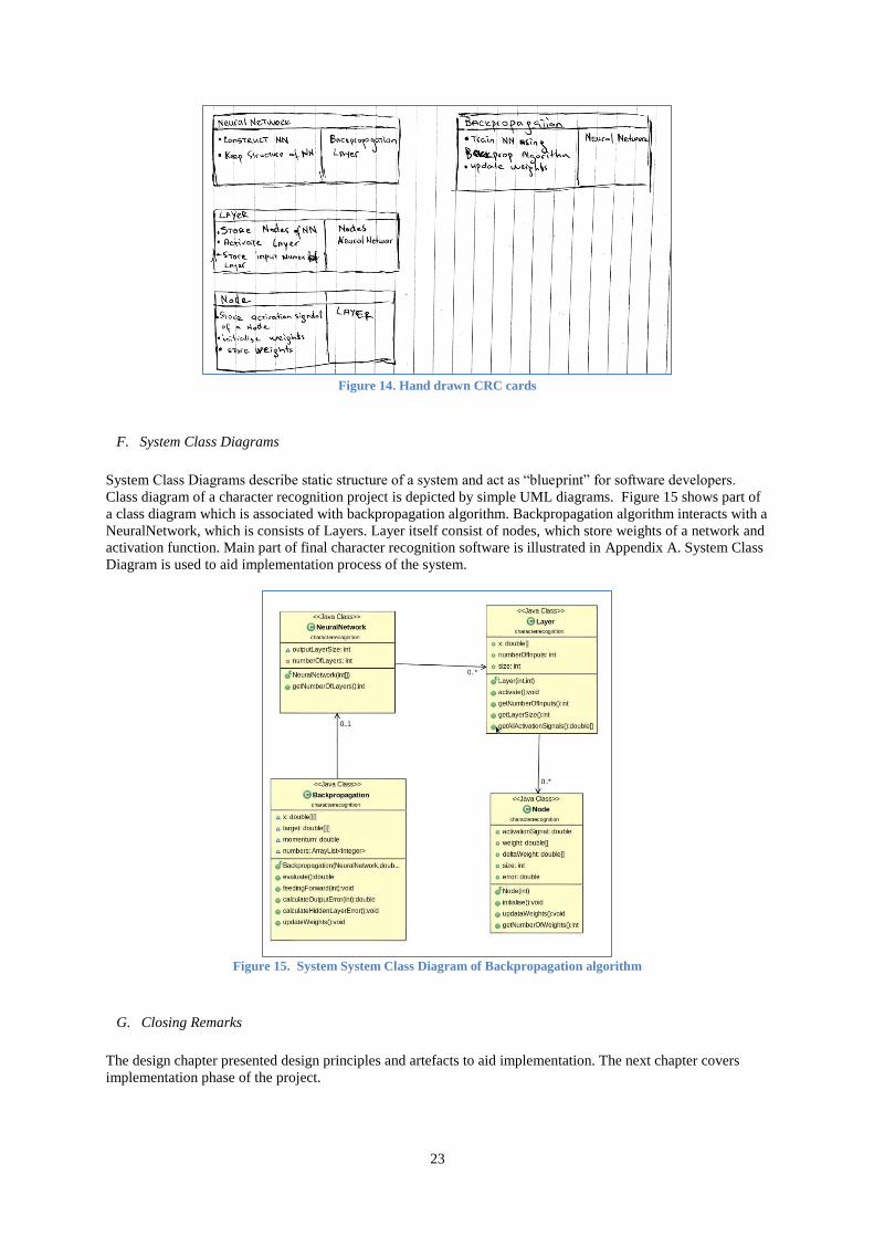
F. System Class Diagrams

System Class Diagrams describe static structure of a system and act as “blueprint” for software developers.

Class diagram of a character recognition project is depicted by simple UML diagrams. Figure 15 shows part of

a class diagram which is associated with backpropagation algorithm. Backpropagation algorithm interacts with a

NeuralNetwork, which is consists of Layers. Layer itself consist of nodes, which store weights of a network and

activation function. Main part of final character recognition software is illustrated in Appendix A. System Class

Diagram is used to aid implementation process of the system.

Figure 15. System System Class Diagram of Backpropagation algorithm

G. Closing Remarks

The design chapter presented design principles and artefacts to aid implementation. The next chapter covers

implementation phase of the project.

24

VI. IMPLEMENTATION

A. Chapter Overview and Introduction

This chapter covers implementation phase of this project. The chapter starts with describing implementation

tools used for development of handwritten character recognition software. The next section encapsulates

evolutionary process of software development through prototypes. Later, Data structure and Algorithms that

were implemented for solving character recognition problem are explicitly described. Techniques used for

improving efficiency of chosen algorithm are highlighted. Final section of this chapter presents walkthrough of

the final system.

B. Implementation Tools

1) Programming Language

The choice of programming language plays a paramount important role in development process of the project.

Development and execution time depends on the programming language used. Application program interface

(API) and libraries allow for fast development of a program by providing building blocks. API is a set of

protocols and tools that are implemented in software applications. Also, considering object oriented approach

undertaken in design process, two object-oriented programming languages were considered for development of

this project; C# and Java.

C# and Java have similar syntaxes and compiled using the state machine; Java Virtual Machine (JVM) and

Common Language Runtime (CLR) respectively. Both programming languages have its advantages and

drawbacks. Since C# was developed after Java it offers more features like supporting unsigned bits and high

precision for decimal arithmetic. Microsoft .Net provides a high number of framework preferences that can be

also used by C# developers. However; C# is a Microsoft technology and has a restricted license for some APIs

and is limited to Microsoft operating systems. Java, on the other hand, can be executed on any operating system

that has installed JVM. Compiled Java code produces bytecode that can be run on any machine. Moreover, Java

Technologies is considered as an open source and has wide library and API choices. Considering portability and

the author’s prior knowledge and experience, Java was selected as a programming language for development of

this project.

2) Development Environment

After programming language was chosen various development environments were considered for implementing

project. Integrated Development Environment (IDE) provides integrated utilities for efficient software

development. It includes compiler, debugger, code editor and code completion features. Some IDEs support

Graphical User Interface (GUI) development by offering simplified GUI construction environment. Developer

can sketch user interface and concentrate on design instead of writing code for GUI that can be seen only after

compiling and running the program.

Eclipse was preferred to as a development environment after considering both multi-language and Java IDEs.

Control over source code, refactoring features, and simple interface make Eclipse one of the best IDEs for Java.

Lack of GUI designer is a main disadvantage of Eclipse. However, facilities provided by Eclipse can be

extended by means of various plugins. Therefore, GUI problem can be eliminated by Windows Builder Pro

plugin which provides drag and drop control mechanism for Eclipse.

C. Prototyping

The first four prototypes were rapid prototypes that were not included in final software. These prototypes were

developed in order to understand various learning algorithms, minimal code was written and only command line

interaction was used. The first prototype involved training single neuron using perceptron learning algorithm in

order to classify OR and AND logic with two binary inputs. For the second prototype, delta rule with linear

activation function was implemented to train single neuron and was tested on OR and AND logic. Delta rule

with non-linear sigmoid activation function was implemented for the third prototype and was compared with

previous prototypes. All of the first three prototypes were unable to fully classify XOR logic due to its non-

25

linear behaviour. For the final rapid prototype, backpropagation algorithm was implemented and this involved

training a multi-layered neural network to learn XOR logic. A multi-layered neural network with one hidden

layer of three neurons could learn XOR logic in a finite number of iterations; the purpose of this prototype was

to understand the behavior of backpropagation algorithm as an improved version of it was used during

development of actual software.

After the main functionalities of backpropagation algorithm was tested by the fourth prototype, and final

software was developed through evolutionary prototypes. Development commenced with implementation of

requirements that have both greater priority and high risk. Requirement with low priority and risk were

implemented during later iterations. GUI was developed at the final stage of development, after the

backpropagation algotihm was implemented and tested. Figure 16 shows main prototypes developed through the

project.

Figure 16. Prototypes developed during implementation of the project.

1) Rapid Prototypes

The first four prototypes were rapid prototypes that were not included in final software. Since these prototypes

were developed in order to understand various learning algorithms, minimal code was written and only

command line interaction was used. The first prototype involved training single neuron using perceptron

learning algorithm. It was trained on OR and AND logic, which had two binary inputs.

For the second prototype, delta rule with linear activation function was implemented to train single neuron and

was also tested on OR and AND logic. Delta rule with non-linear sigmoid activation function was implemented

for the third prototype and was compared with previous prototype. All of the first three prototypes were unable

to fully classify XOR logic due to its non-linear behavior.

For final rapid prototype backpropagation algorithm was implemented. It involved training multi-layered neural

network to learn XOR logic. Multi-layered neural network with one hidden layer of three neurons could learn

XOR logic. Purpose of this prototype was to understand behavior of backpropagation algorithm since improved

version of it was used during development of actual software.

2) Evolutionary Prototypes

After main functionalities of bacpropagation algorithm was tested by the forth prototype, final software was

developed throughout time-boxed iterations. Evolutionary prototype, which implemented chosen requirements,

was produced at the end of the each iteration. Requirements were chosen according to risk and priority analysis

of functional requirements (Table 2). Development commenced with implementation of requirements that have

greater priority and high risk. Requirement with low priority and risk were implemented at later iterations.

Graphical user interface (GUI) was developed at the final stage of development, after backpropagation algotihm

was implemented and tested.

26

D. Algorithmics and Data Structure

Final software, which was built through multiple prototypes, can recognise handwritten characters using neural

network. This section outlines data structure and algorithm that were used in implementation of the final system.

1) Data Structure

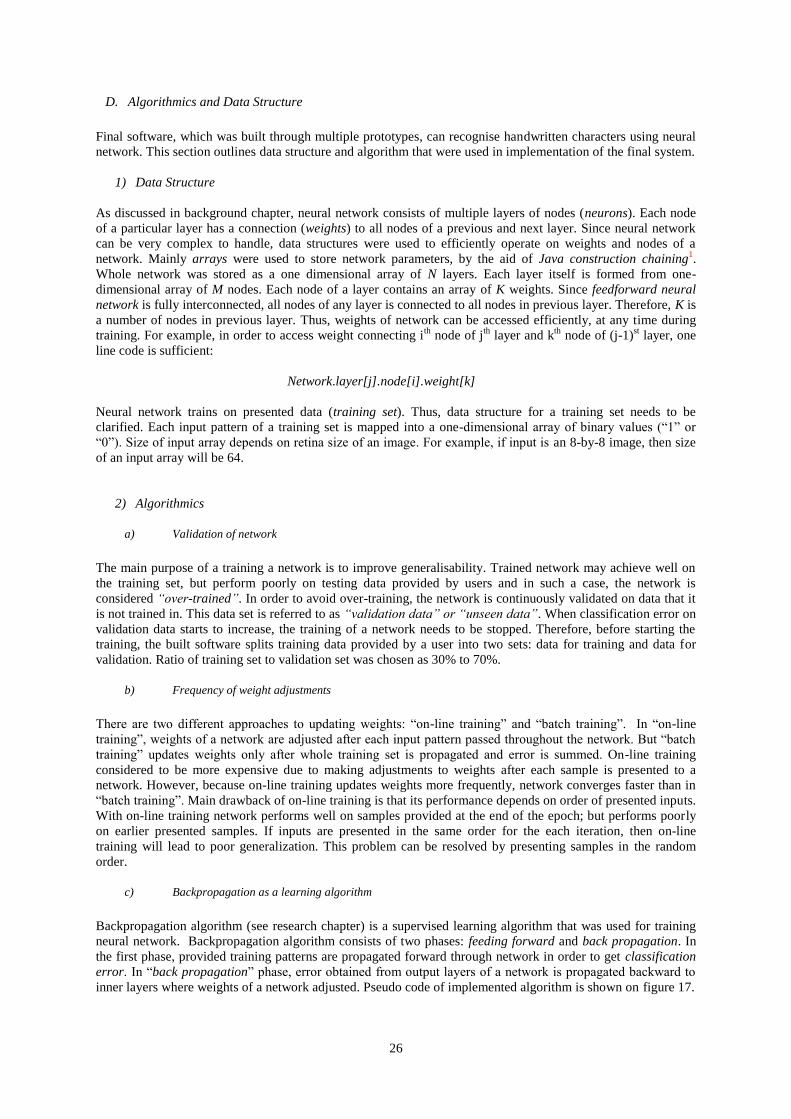
As discussed in background chapter, neural network consists of multiple layers of nodes (neurons). Each node

of a particular layer has a connection (weights) to all nodes of a previous and next layer. Since neural network

can be very complex to handle, data structures were used to efficiently operate on weights and nodes of a

network. Mainly arrays were used to store network parameters, by the aid of Java construction chaining1.

Whole network was stored as a one dimensional array of N layers. Each layer itself is formed from one-

dimensional array of M nodes. Each node of a layer contains an array of K weights. Since feedforward neural

network is fully interconnected, all nodes of any layer is connected to all nodes in previous layer. Therefore, K is

a number of nodes in previous layer. Thus, weights of network can be accessed efficiently, at any time during

training. For example, in order to access weight connecting ith

node of jth

layer and kth

node of (j-1)st layer, one

line code is sufficient:

Network.layer[j].node[i].weight[k]

Neural network trains on presented data (training set). Thus, data structure for a training set needs to be

clarified. Each input pattern of a training set is mapped into a one-dimensional array of binary values (“1” or

“0”). Size of input array depends on retina size of an image. For example, if input is an 8-by-8 image, then size

of an input array will be 64.

2) Algorithmics

a) Validation of network

The main purpose of a training a network is to improve generalisability. Trained network may achieve well on

the training set, but perform poorly on testing data provided by users and in such a case, the network is

considered “over-trained”. In order to avoid over-training, the network is continuously validated on data that it

is not trained in. This data set is referred to as “validation data” or “unseen data”. When classification error on

validation data starts to increase, the training of a network needs to be stopped. Therefore, before starting the

training, the built software splits training data provided by a user into two sets: data for training and data for

validation. Ratio of training set to validation set was chosen as 30% to 70%.

b) Frequency of weight adjustments

There are two different approaches to updating weights: “on-line training” and “batch training”. In “on-line

training”, weights of a network are adjusted after each input pattern passed throughout the network. But “batch

training” updates weights only after whole training set is propagated and error is summed. On-line training

considered to be more expensive due to making adjustments to weights after each sample is presented to a

network. However, because on-line training updates weights more frequently, network converges faster than in

“batch training”. Main drawback of on-line training is that its performance depends on order of presented inputs.

With on-line training network performs well on samples provided at the end of the epoch; but performs poorly

on earlier presented samples. If inputs are presented in the same order for the each iteration, then on-line

training will lead to poor generalization. This problem can be resolved by presenting samples in the random

order.

c) Backpropagation as a learning algorithm

Backpropagation algorithm (see research chapter) is a supervised learning algorithm that was used for training

neural network. Backpropagation algorithm consists of two phases: feeding forward and back propagation. In

the first phase, provided training patterns are propagated forward through network in order to get classification

error. In “back propagation” phase, error obtained from output layers of a network is propagated backward to

inner layers where weights of a network adjusted. Pseudo code of implemented algorithm is shown on figure 17.

27

Training starts with initialising weights (between -1 and 1). However, weights with large values can saturate

input sample, which increases convergence time of network. Therefore weights of a network are initialised by

gaussian function which ensures that most of the weights are close to zero. Once weights are initialised, network

starts training on training data using backpropagation algorithm.

The training data set is shuffled before each training epoch. For each training epoch, weights of a neural

network are adjusted after each input pattern (vector) of a shuffled training set is classified by the network.

Errors in classification of training samples are summed in order to obtain a total error of the training epoch. The

training process continues until the total epoch of training epoch is less than expected minimal error. If minimal

error is never achieved, then training can continue forever. Therefore, in order to avoid infinite training, the

training process is halted whenever user decides terminate training. When a training epoch ends, the network is

tested on validation data in order to prevent over-training.

Figure 17. Hihh level pseudo code of backpropagation algorithm implemented in the final system

E. Walkthrough

Final version of software developed by author is demonstrated in Appendix B. Process of setting up neural

network, training neural network and testing character recognition capabilities of software is depicted through

captions. Hierarchical Task Analysis (HTA) diagram aids flow of functionalities provided by developed

software.

F. Concluding Remarks

This chapter covered implementation phase of the project. The next chapter presents experimental results

achieved throughout analysis of the software.

28

VII. RESULTS

A. Chapter Overview

This chapter encapsulates performance analysis of the developed software. Experiments were conducted in

order to study influence of neural network construction and training parameters on recognition capabilities of

the system.

B. Final Results

Since the final system was developed throughout evolutionary prototypes, number of distinct classes that system

was trained and tested was incrementing. Firstly, network was trained and tested on two distinct classes; then

four, six, eight; and finally on ten distinct classes. Figure 18 shows classification rate of the neural network

depending on the number of distinct classes. Classification rate is a percentage of correctly classified samples.

Despite neural network is training well on training data, error rate on validation data set shows how well neural

network is generalised. Based on the results, it can be deducted that classification rate decreases when number

of distinct classes grow.

Figure 18. Classification Rate.

C. Parameter Analysis of the Backpropagation algorithm

An ability of bacpropagation algorithm to learn on training data depends on chosen training parameters.

Sensitivity analysis was undertaken in order to understand relationship between training parameters and training

process of a system. Sensitivity analysis involves examining behavior of a system by changing training

parameters of a backpropagation algorithm and network topology.

For final software, neural network was trained on 200 training samples of each digit. Retina size of each input

pattern was 16x16. By varying learning rate, momentum and network topology at a time, network was trained

and validated for each set of parameters.

100 100 100 100 99

97.5 97

96 95.5

91.5

2 4 6 8 10

Cla

sifi

cati

on

Rat

e

Number of Classes

Training Data Validation Data

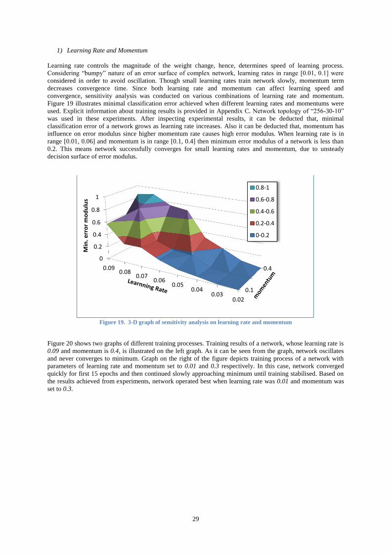
29

1) Learning Rate and Momentum

Learning rate controls the magnitude of the weight change, hence, determines speed of learning process.

Considering “bumpy” nature of an error surface of complex network, learning rates in range [0.01, 0.1] were

considered in order to avoid oscillation. Though small learning rates train network slowly, momentum term

decreases convergence time. Since both learning rate and momentum can affect learning speed and

convergence, sensitivity analysis was conducted on various combinations of learning rate and momentum.

Figure 19 illustrates minimal classification error achieved when different learning rates and momentums were

used. Explicit information about training results is provided in Appendix C. Network topology of “256-30-10”

was used in these experiments. After inspecting experimental results, it can be deducted that, minimal

classification error of a network grows as learning rate increases. Also it can be deducted that, momentum has

influence on error modulus since higher momentum rate causes high error modulus. When learning rate is in

range [0.01, 0.06] and momentum is in range [0.1, 0.4] then minimum error modulus of a network is less than

0.2. This means network successfully converges for small learning rates and momentum, due to unsteady

decision surface of error modulus.

Figure 19. 3-D graph of sensitivity analysis on learning rate and momentum

Figure 20 shows two graphs of different training processes. Training results of a network, whose learning rate is

0.09 and momentum is 0.4, is illustrated on the left graph. As it can be seen from the graph, network oscillates

and never converges to minimum. Graph on the right of the figure depicts training process of a network with

parameters of learning rate and momentum set to 0.01 and 0.3 respectively. In this case, network converged

quickly for first 15 epochs and then continued slowly approaching minimum until training stabilised. Based on

the results achieved from experiments, network operated best when learning rate was 0.01 and momentum was

set to 0.3.

0.020.03

0.040.05

0.060.07

0.080.09

0

0.2

0.4

0.6

0.8

1

0.1

0.4

Min

. err

or

mo

du

lus

0.8-1

0.6-0.8

0.4-0.6

0.2-0.4

0-0.2

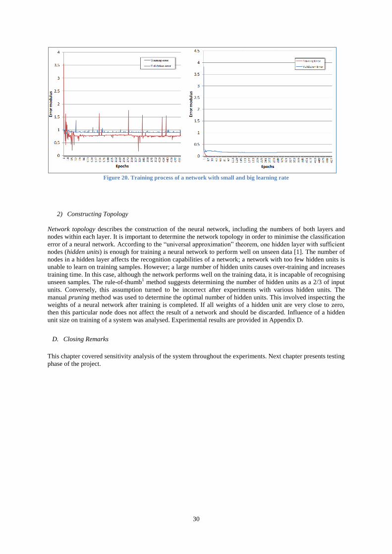
30

Figure 20. Training process of a network with small and big learning rate

2) Constructing Topology

Network topology describes the construction of the neural network, including the numbers of both layers and

nodes within each layer. It is important to determine the network topology in order to minimise the classification

error of a neural network. According to the “universal approximation” theorem, one hidden layer with sufficient

nodes (hidden units) is enough for training a neural network to perform well on unseen data [1]. The number of

nodes in a hidden layer affects the recognition capabilities of a network; a network with too few hidden units is

unable to learn on training samples. However; a large number of hidden units causes over-training and increases

training time. In this case, although the network performs well on the training data, it is incapable of recognising

unseen samples. The rule-of-thumb1 method suggests determining the number of hidden units as a 2/3 of input

units. Conversely, this assumption turned to be incorrect after experiments with various hidden units. The

manual pruning method was used to determine the optimal number of hidden units. This involved inspecting the

weights of a neural network after training is completed. If all weights of a hidden unit are very close to zero,

then this particular node does not affect the result of a network and should be discarded. Influence of a hidden

unit size on training of a system was analysed. Experimental results are provided in Appendix D.

D. Closing Remarks

This chapter covered sensitivity analysis of the system throughout the experiments. Next chapter presents testing

phase of the project.

31

VIII. TESTING

A. Chapter Overview

This chapter covers testing process applied, in order to validate and verify built software.

B. Introduction to Software Testing

Testing is the process of verifying whether software meets identified requirements. Any flows in a system, bugs

in code and inconsistency of requirements are revealed by testing. Therefore, testing is an important phase to

complete, in order to present robust product. Start of a testing phase depends on chosen software development

model. For waterfall model testing starts when development phase is finished. However, in agile methodology,

which was chosen as a development model for this project, testing is done after the each iteration. Therefore,

faults in a system exposed in early stages of the development and can be eliminating without additional cost

[51]. Two types of testing were used in this project: “black-box testing” and “white-box testing”.

1) Black Box Testing

Black box testing is a testing technique used to test functionality of a system without knowing its interior

structure. System is approached by using user interface or command line. System is checked for inconsistent

behavior throughout simulation with various parameters. This method can also referred to as “hacking” or

“exhaustive input testing” [52]. Black box testing can also be performed by users who do not have any

programming experience, since code is not accessed. Graphical user interface (GUI) of character recognition

system was tested by black box testing method. Each input condition was simulated in order to see whether GUI

responds correctly. Acceptance and System testing are examples of such testing methods.

2) White Box Testing

Internal structure of a system is tested by a white box testing method. Source code is inspected in order to find

vulnerable pieces of code. As prototype evolves, late discovery of small bugs in a code fragment can lead to

spending more time on finding an error. Therefore, frequent white box testing is encouraged [53]. White box

testing was used throughout project for testing of incremental prototypes.

32

IX. EVALUATION AND CONCLUSION

A. Chapter Overview and Introduction

This chapter aims to conclude report with a summary and evaluation of a project. The chapter outlines areas for

improvement.

This project required building a software system that could recognise handwritten characters using neural

network. Whole life-cycle of a project development was undertaken according to agile software development

methodologies. All requirements were identified, forming functional and non-functional requirements table

(Table 2 and Table 3). System was designed using design principles and patterns. Class diagrams were created

in order to aid implementation process of the final system. Since agile software development encourages

iterative and incremental development, final software was built through evolutionary and rapid prototypes

(Figure 16). Initial prototypes involved building simple prototypes of a neural network that were using various

learning algorithms to train. Since these prototypes were developed for investigating behavior of simple learning

algorithms, they were not used in the final development of the system. Later, final system implementing

complex learning algorithm (backpropagation) was developed. Final system involved building graphical user

interface that allows user to identify structure and parameters of neural network. Created neural network trained

itself to recognise set of characters of presented classes.

B. Project Evaluation

Overall, project was successfully completed as all functional and non-functional requirements (Table 2 and

Table 3), were implemented and tested. However, final software was not tested on full character range. It was

due to the absence of free source for sufficient number of handwritten character samples. Also, training was

growing as number of distinct classes increase. Neural network, which implemented in final system, were

trained, tested and analysed on 0 to 9 digits. Final results show that network successfully trains on given

samples of digits, since error on validation set was around 10%. Highly flexibly software was developed for a

final product. Training process and results depend on training parameters and network structure. Therefore, built

software can be used for learning behavior of artificial neural network.

C. Further Improvements

Despite successfully achieved results, there are still areas for improvement. Both pre-processing and feature

extraction can be inspected to improve classification rate of a network. For example, given a set of training

samples, software can automatically extend training samples by adding new samples to presented set. New

samples will be distorted, blurred or contain noise. This process can improve generalizability of a network.

Also, input image provided by the user can be passes pre-processing in order to get clear image.

Furthermore, dependency of learning process on structure and parameters of a network can be studied further.

Rather than manually setting number of hidden layers and units of a neural network, net pruning can optimise

structure of a network automatically while training. Moreover, it would be interesting to investigate hopfield

network and try out reinforcement learninig.

Finally, research of algorithms for speeding up learning process is essential for reducing computational time for

large networks. Methods such as quickprop algorithm and conjugate gradient method reduce convergence time

of a network.

D. Concluding Remarks

This chapter finalised report on character recognition software. Summary of a project with brief development

process was outlined. Project was evaluated and further improvements were highlighted.

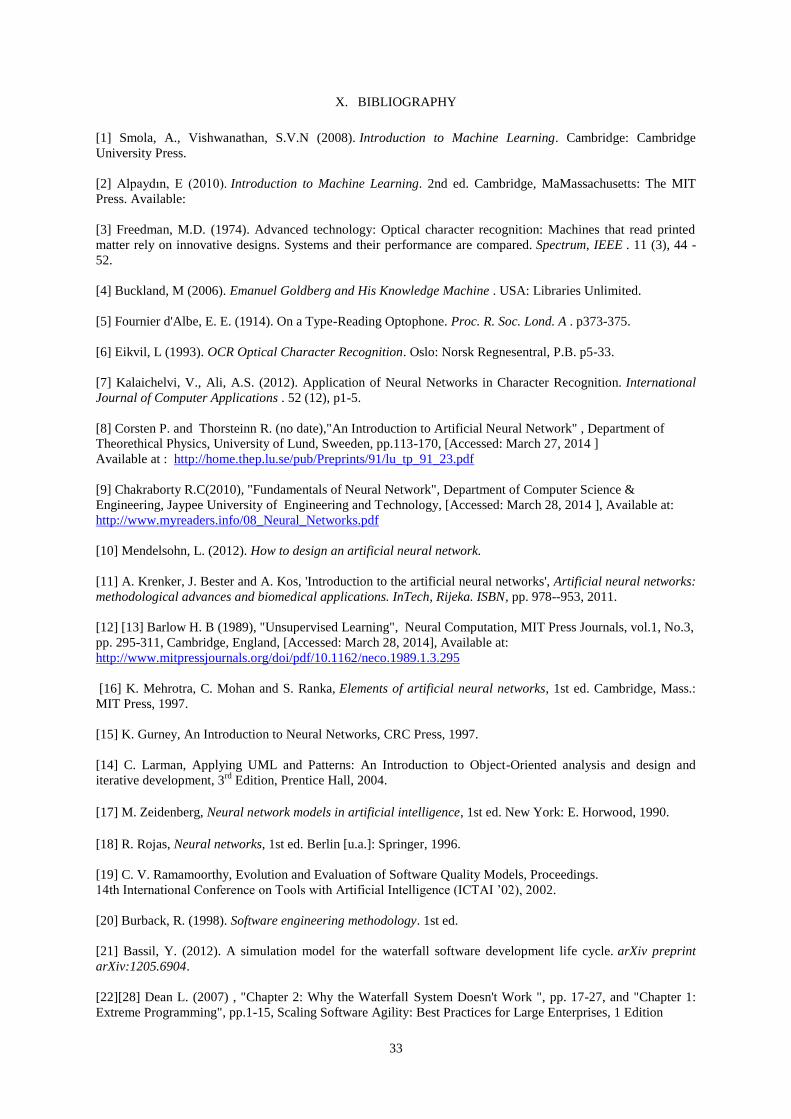
33

X. BIBLIOGRAPHY

[1] Smola, A., Vishwanathan, S.V.N (2008). Introduction to Machine Learning. Cambridge: Cambridge

University Press.

[2] Alpaydın, E (2010). Introduction to Machine Learning. 2nd ed. Cambridge, MaMassachusetts: The MIT

Press. Available:

[3] Freedman, M.D. (1974). Advanced technology: Optical character recognition: Machines that read printed

matter rely on innovative designs. Systems and their performance are compared. Spectrum, IEEE . 11 (3), 44 -

52.

[4] Buckland, M (2006). Emanuel Goldberg and His Knowledge Machine . USA: Libraries Unlimited.

[5] Fournier d'Albe, E. E. (1914). On a Type-Reading Optophone. Proc. R. Soc. Lond. A . p373-375.

[6] Eikvil, L (1993). OCR Optical Character Recognition. Oslo: Norsk Regnesentral, P.B. p5-33.

[7] Kalaichelvi, V., Ali, A.S. (2012). Application of Neural Networks in Character Recognition. International

Journal of Computer Applications . 52 (12), p1-5.

[8] Corsten P. and Thorsteinn R. (no date),"An Introduction to Artificial Neural Network" , Department of

Theorethical Physics, University of Lund, Sweeden, pp.113-170, [Accessed: March 27, 2014 ]

Available at : http://home.thep.lu.se/pub/Preprints/91/lu_tp_91_23.pdf

[9] Chakraborty R.C(2010), "Fundamentals of Neural Network", Department of Computer Science &

Engineering, Jaypee University of Engineering and Technology, [Accessed: March 28, 2014 ], Available at: http://www.myreaders.info/08_Neural_Networks.pdf

[10] Mendelsohn, L. (2012). How to design an artificial neural network.

[11] A. Krenker, J. Bester and A. Kos, 'Introduction to the artificial neural networks', Artificial neural networks:

methodological advances and biomedical applications. InTech, Rijeka. ISBN, pp. 978--953, 2011.

[12] [13] Barlow H. B (1989), "Unsupervised Learning", Neural Computation, MIT Press Journals, vol.1, No.3,

pp. 295-311, Cambridge, England, [Accessed: March 28, 2014], Available at: http://www.mitpressjournals.org/doi/pdf/10.1162/neco.1989.1.3.295

[16] K. Mehrotra, C. Mohan and S. Ranka, Elements of artificial neural networks, 1st ed. Cambridge, Mass.:

MIT Press, 1997.

[15] K. Gurney, An Introduction to Neural Networks, CRC Press, 1997.

[14] C. Larman, Applying UML and Patterns: An Introduction to Object-Oriented analysis and design and

iterative development, 3rd

Edition, Prentice Hall, 2004.

[17] M. Zeidenberg, Neural network models in artificial intelligence, 1st ed. New York: E. Horwood, 1990.

[18] R. Rojas, Neural networks, 1st ed. Berlin [u.a.]: Springer, 1996.

[19] C. V. Ramamoorthy, Evolution and Evaluation of Software Quality Models, Proceedings.

14th International Conference on Tools with Artificial Intelligence (ICTAI ’02), 2002.

[20] Burback, R. (1998). Software engineering methodology. 1st ed.

[21] Bassil, Y. (2012). A simulation model for the waterfall software development life cycle. arXiv preprint

arXiv:1205.6904.

[22][28] Dean L. (2007) , "Chapter 2: Why the Waterfall System Doesn't Work ", pp. 17-27, and "Chapter 1:

Extreme Programming", pp.1-15, Scaling Software Agility: Best Practices for Large Enterprises, 1 Edition

http://home.thep.lu.se/pub/Preprints/91/lu_tp_91_23.pdf

http://www.myreaders.info/08_Neural_Networks.pdf

http://www.mitpressjournals.org/doi/pdf/10.1162/neco.1989.1.3.295

34

[23] Petersen, K., Wohlin, C. and Baca, D. (2009). The waterfall model in large-scale development. Springer,

pp.386--400.

[24] Agilemanifesto.org, (2014). Manifesto for Agile Software Development. [online] Available at:

http://agilemanifesto.org/ [Accessed 18 Mar. 2014].

[25] Warsta, J. (2002). Agile Software Development Methods: Review and Analysis. 1st ed. Oulu: VTT.

[26] Schwaber, K. and Beedle, M. (2002). Agile software development with Scrum. 1st ed. Upper Saddle River,

NJ: Prentice Hall.

[27] Sharma, S., Sarkar, D. and Gupta, D. (2012). Agile Processes and Methodologies: A Conceptual

Study. International Journal on Computer Science \& Engineering, 4(5).

[29] Beck, K. (2000). Extreme programming eXplained. 1st ed. Reading, MA: Addison-Wesley.

[30] Macaulay, L. (1996). Requirements engineering. 1st ed. London: Springer.

[31] Kotonya, G. and Sommerville, I. (1998) Requirements Engineering: processes and techniques, John Wiley.

[32] Alexander Kossiakof, William N. Sweet (2011). Systems Engineering: Principles and Practices.

[33] Dennis, A., Wixom, B.H. and Roth, R.M. (2006). Systems Analysis and Design. 3rd ed. Hoboken: Johniley

& Sons, Inc.

[34] Richard Vidgen. Requirements analysis and UML.

[35] Craig Larman. Applying UML and Patterns. Prentice Hall, 2004.

[36] Vincent Rainardi. Building a Data Warehouse: With Examples in SQL Server (2008).

[37] Sommerville Ian. Software Engineering, 7th ed. (2006).

[38] Pekka A., Richard B., Kieran C., Brian F., Lorraine M., Xiaofeng W., Agile Processes in Software

Engineering and Extreme Programming (2008)

[39] Aybüke A. and Claes W. (2005) Engineering and Managing Software Requirements

[40] Murali Chemuturi, Requirements Engineering and Management for Software Development Projects

[41] Frank Maurer and Don Wells. Extreme Programming and Agile Methods – XP/Agile Universe 2003 (2003)

[42] Wikipedia, (2014). Stakeholder analysis. [online] Available at:

http://en.wikipedia.org/wiki/Stakeholder_analysis [Accessed 11 Mar. 2014].

[43] Stuart B. (2011), "The system Engineering Tool Box", Burge Hughes Walsh, [Accessed: March 30, 2014],

Available at: http://www.burgehugheswalsh.co.uk/uploaded/documents/CD-Tool-Box-V1.0.pdf

[44] Craig Larman. Applying UML and Patterns. Prentice Hall, 2004.

[45] Centre for Information Technology and Engineering, Manonmaniam Sundaranar University. Software

Engineering concepts and implementation.

[46] David Embrey. Task analysis techniques.

[47] Anne E. Adams, Wendy A. Rogers and Arthur D. Fisk. Ergonomics in design: the quarterly of human

factors applications. 2012

[48] Bible R, Noble J, Tempero E, Reflection on CRC cards and OO Design

http://www.burgehugheswalsh.co.uk/uploaded/documents/CD-Tool-Box-V1.0.pdf

35

[49] Börstler, J, Schulte, C. Teaching object oriented modelling with CRC-Cards and roleplaying games

[50] Connell, J. and Shafer, L. (1995). Object-oriented rapid prototyping. 1st ed. Englewood Cliffs, N.J.:

Yourdon Press.

[51] John E.B., Wachovia B. and Charlotte NC.(2003-2004), "Software Testing Fundamentals- Concepts, Roles

and Terminology", SAS Software, [Accessed: April 2, 2014], Available at:

http://www2.sas.com/proceedings/sugi30/141-30.pdf

[52] Myers, G., Sandler, C. and Badgett, T. (2012). The art of software testing. 2nd ed. Hoboken, N.J.: John

Wiley & Sons.

http://www2.sas.com/proceedings/sugi30/141-30.pdf

36

XI. APPENDIX A

Figure 21. System Class Diagram of core character recognition system

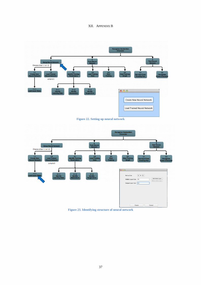
37

XII. APPENDIX B

Figure 22. Setting up neural network

Figure 23. Identifying structure of neural network

38

Figure 24. Loading already trained network

Figure 25. Indentifying training parameters

39

Figure 26. Loading training data for the training

Figure 27. Starting the training

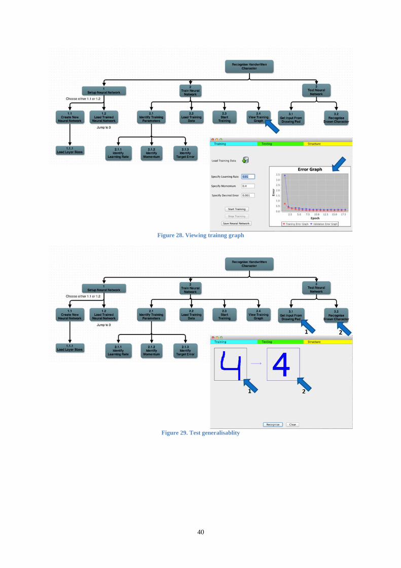
40

Figure 28. Viewing trainng graph

Figure 29. Test generalisablity

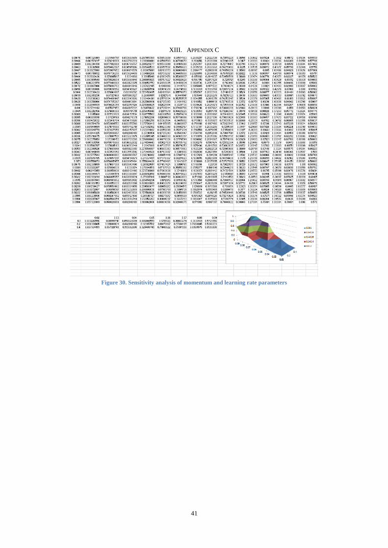
41

XIII. APPENDIX C

Figure 30. Sensitivity analysis of momentum and learning rate parameters

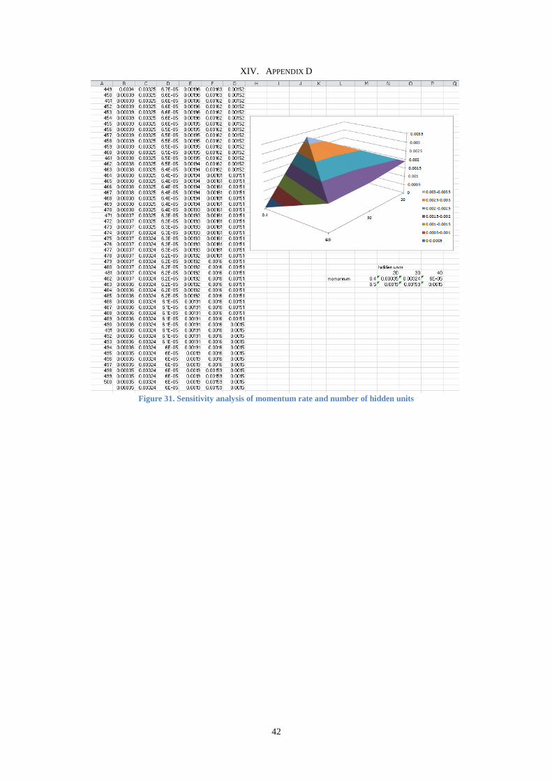
42

XIV. APPENDIX D

Figure 31. Sensitivity analysis of momentum rate and number of hidden units

Character Recognition using Artificial Neural...

Documents

Transcript of Character Recognition using Artificial Neural...