Chapter 4

Experiment 2:Equipotentials and Electric Fields

4.1 Introduction

One way to look at the force between charges is to say that the charge alters the space aroundit by generating an electric field E. Any other charge placed in this field then experiences aCoulomb force. We thus regard the E field as transmitting the Coulomb force.

To define the electric field, E, more precisely, consider a small positive test charge q at agiven location. As long as everything else stays the same, the Coulomb force exerted on thetest charge q is proportional to q. Then the force per unit charge, F/q, does not depend onthe charge q, and therefore can be regarded meaningfully to be the electric field E at thatpoint.

In defining the electric field, we specify that the test charge q be small because in practicethe test charge q can indirectly affect the field it is being used to measure. If, for example,we bring a test charge near the Van de Graaff generator dome, the Coulomb forces from thetest charge redistribute the charge on the conducting dome and thereby slightly change theE field that the dome produces. But secondary effects of this sort have less and less effecton the proportionality between F and q as we make q smaller.

So many phenomena can be explained in terms of the electric field, but not nearly aswell in terms of charges simply exerting forces on each other through empty space, thatthe electric field is regarded as having a real physical existence, rather than being a meremathematically-defined quantity. For example when a collection of charges in one region ofspace move, the effect on a test charge at a distant point is not felt instantaneously, butinstead is detected with a time delay that corresponds to the changed pattern of electricfield values moving through space at the speed of light.

Closely associated with the concept of electric field is the pictorial representation of thefield in terms of lines of force. These are imaginary geometric lines constructed so thatthe direction of the line, as given by the tangent to the line at each point, is always in thedirection of the E field at that point, or equivalently, is in the direction of the force thatwould act on a small positive test charge placed at that point. The electric field and the

43

CHAPTER 4: EXPERIMENT 2

concept of lines of electric force can be used to map out what forces act on a charge placedin a particular region of space.

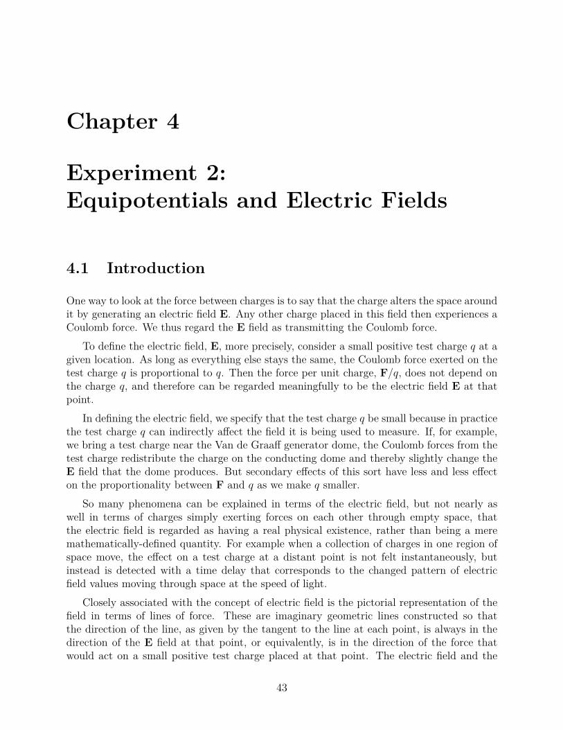
Figures 4.1(a) and 4.1(b) show a region of space around an electric dipole, with theelectric field indicated by lines of force. The charges in Figure 4.1(a) are identical butopposite in sign. In Figure 4.1(b) the charges have the same sign. Above each figure is apicture of a region around charges in which grass seed has been sprinkled on a glass plate.The elongated seeds have aligned themselves with the electric field at each location, thusindicating its direction at each point.

(a) (b)

Figure 4.1: Above: Grass seeds alignthemselves with the electric field between twocharges. Below: The drawing shows thelines of force associated with the electric fieldbetween charges. (a) shows a charge pairwith negative charge above and positive chargebelow. (b) shows two positive charges.

A few simple rules govern the behaviorof electric field lines. These rules can beapplied to deduce some properties of thefield for various geometrical distributions ofcharge:

1) Electric field lines are drawn such thata tangent to the line at a particularpoint in space gives the direction of theelectrical force on a small positive testcharge placed at the point.2) The density of electric field lines in-dicates the strength of the E field in aparticular region. The field is strongerwhere the lines get closer together.

3) Electric field lines start on positivecharges and end on negative charges.Sometimes the lines take a long routearound and we can only show a portionof the line within a diagram of the kindbelow. If net charge in the picture is notzero, some lines will not have a chargeon which to end. In that case theyhead out toward infinity, as shown inFigure 4.1(b).You might think when several charges are present that the electric field lines from two

charges could meet at some location, producing crossed lines of force. But imagine placing acharge where the two lines intersect. Charges are never confused about the direction of theforce acting on them, so along which line would the force lie? In such a case, the electricfields add vectorially at each point, producing a single net E field that lies along one specificline of force, rather than being at the intersection of two lines of force. Thus, it can be seenthat none of the lines cross each other. It can also be shown that two field lines never mergeto become one.

44

CHAPTER 4: EXPERIMENT 2

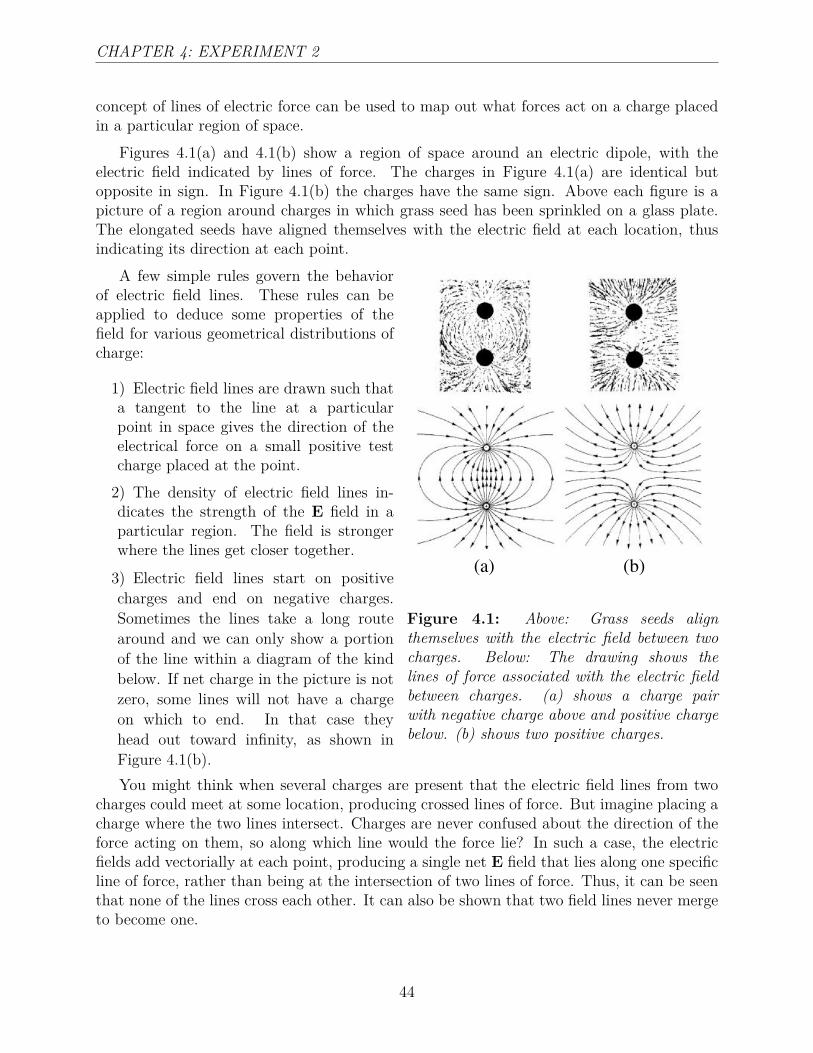
Figure 4.2: Electric field around a group ofcharges. Lines of force are shown as solidlines. Equipotential lines are shown as dashedlines.

Under certain circumstances, the rulesdefining these field lines can be used to de-duce some general properties of charges andtheir forces. For example, a property easilydeduced from these rules is that a region ofspace enclosed by a spherically symmetricdistribution of charge has zero electric fieldeverywhere within that region (assumingno additional charges produce electric fieldsinside). Imagine first a spherically sym-metric thin shell of positive charge all ata certain distance from the center. Fieldlines from the shell would have to be radiallyoutward equally in all directions. If theseoutward pointing lines continued radiallyinward beneath the shell, they would havenowhere to end. Hence, the field lines musthave ended at the surface charge, and there

must be zero field everywhere inside. Next, suppose the spherically symmetric distributionof charge surrounding the uncharged region is not merely a thin shell. We can neverthelessconsider the charge distribution to be divided up into many thin layers each at a differentradius. Each layer contributes its own field lines that end at that layer, producing none ofthe field lines in the region enclosed by that layer. Then any point in the region of interestis inside all of the thin layers, where all the field lines have ended. We can conclude thatthe E field is zero at any point within a region surrounded by the spherical distribution ofcharge.

In Figures 4.1(a) and 4.1(b) it is seen that the density of field lines is greater near thecharges because the lines must converge closer together as they approach a particular charge.It can also be shown that the electric field intensity increases near conducting surfaces thatare curved to protrude outward, so that they have a positive curvature. Curvature is definedas the inverse of the radius. A flat surface has zero curvature. A needle point has a verysmall radius and a large positive curvature. The larger the curvature of a conducting surface,the greater the field intensity is near the surface.

CheckpointWhat are three properties of electric lines of force? Why do electric lines of force nevercross?

CheckpointHow do the electric lines of force represent an increasing field intensity?

45

CHAPTER 4: EXPERIMENT 2

CheckpointHow can you prove from properties of electric field lines that a spherical distributionof charge surrounding an uncharged region produces no electric field anywhere withinthe region?

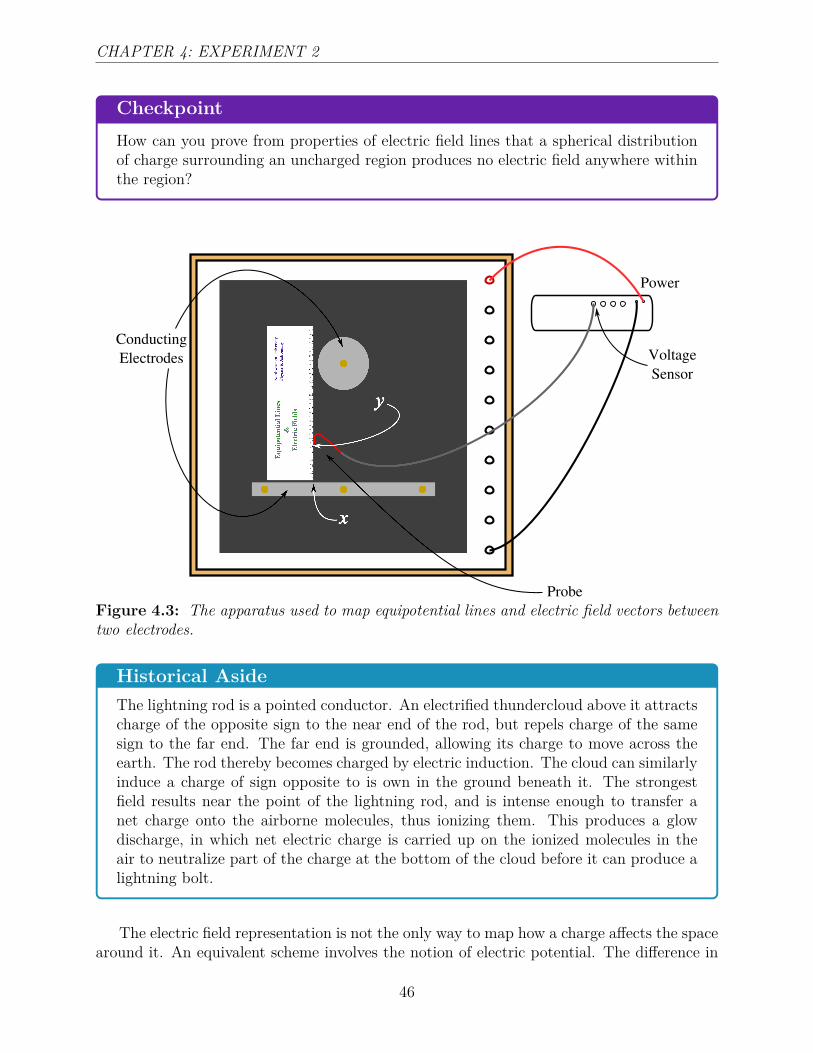
Conducting

Electrodes

Power

Voltage

Sensor

Probe

Figure 4.3: The apparatus used to map equipotential lines and electric field vectors betweentwo electrodes.

Historical AsideThe lightning rod is a pointed conductor. An electrified thundercloud above it attractscharge of the opposite sign to the near end of the rod, but repels charge of the samesign to the far end. The far end is grounded, allowing its charge to move across theearth. The rod thereby becomes charged by electric induction. The cloud can similarlyinduce a charge of sign opposite to is own in the ground beneath it. The strongestfield results near the point of the lightning rod, and is intense enough to transfer anet charge onto the airborne molecules, thus ionizing them. This produces a glowdischarge, in which net electric charge is carried up on the ionized molecules in theair to neutralize part of the charge at the bottom of the cloud before it can produce alightning bolt.

The electric field representation is not the only way to map how a charge affects the spacearound it. An equivalent scheme involves the notion of electric potential. The difference in

46

CHAPTER 4: EXPERIMENT 2

electric potential between two points A and B is defined as the work per unit charge requiredto move a small positive test charge from point A to point B against the electric force. Forelectrostatic forces, it can be shown that this work depends only on the locations of thepoints A and B and not on the path followed between them in doing the work. Therefore,choosing a convenient point in the region and arbitrarily assigning its electric potential tohave some convenient value specifies the electric potential at every other point in the regionas the work per unit test charge done to move a test charge between the points. It is usualto choose either some convenient conductor or else the ground as the reference, and to assignit a potential of zero.

General InformationThis bears some similarity to how the gravitational potential energy was defined. Wecould have considered the “electric potential energy” of a test charge in analogy withthe gravitational potential energy by considering the work, not the work per unitcharge, done in moving a test charge between two points. But just as the gravitationalpotential energy itself cannot be used to characterize the gravitational field because itdepends on the test mass used, the electric potential energy similarly depends on thetest charge used.

But the force and therefore the work to move the test charge from one location to anotheris proportional to its charge. Thus the work per unit charge, or electric potential difference,is independent of the test charge used as long as the field does not vary in time, so that theelectric potential characterizes the electric field itself throughout the region of space withoutregard to the magnitude of the test charge used to probe it.

It is convenient to connect points of equal potential with lines in two dimensional prob-lems; or surfaces in the case of three dimensions. These lines are called equipotential lines;these surfaces are called equipotential surfaces; volumes, surfaces, or lines whose points allhave the same electric potential are called equipotentials.

If a small test charge is moved so that its direction of motion is always perpendicular tothe electric field at each location, then the electric force and the direction of motion at eachpoint are perpendicular. No work is done against the electric force, and the potential ateach point traversed is therefore the same. Hence a path traced out by moving in a directionperpendicular to the electric field at each point is an equipotential.

Conversely, if the test charge is moved along an equipotential, there is no change inpotential and therefore no work done on the charge by the electric field. For non-zeroelectric field this can happen only if the charge is being moved perpendicular to the field ateach point on such a path. Therefore, electric field lines and equipotentials always cross atright angles.

Figure 4.2 shows a region of space around a group of charges. The electric lines offorce are indicated with solid lines and arrows. The electric field can also be indicated byequipotential lines, shown as dashed lines in the figure. The mapping of a region of space

47

CHAPTER 4: EXPERIMENT 2

with equipotential lines or, in the case of 3-D space, with equipotential surfaces, providesthe same degree of information as by mapping out the electric field itself throughout theregion.

CheckpointAre the electric field representation and the equipotential line representation equivalentin terms of how much information they contain about the electric field?

4.2 Theory

Recall that the work done by the electric force, F, in moving the charge from point a topoint b is given by

Wab =∫ b

aF · dr, (4.1)

where dr is a small piece of the path traveled from a to b. We can write this in terms ofthe electric field; if our charge is q, then F = qE and

Wab =∫ b

aqE · dr = q

∫ b

aE · dr. (4.2)

Because of this we also find it convenient to talk about the work per unit charge

Vab = Wab

q=∫ b

aE · dr . (4.3)

Since the electric force is conservative, we also find it convenient to introduce a potentialenergy function, U(x, y, z), and a potential energy per unit charge function; we call this thepotential function, V (x, y, z) = U/q, and define its units to be the Volt (1V = 1 J/C). Wedefine U(x, y, z) in such a way that total energy is conserved. Since work is a change inkinetic energy, it must correspond to an opposite change in potential energy if the total isto remain constant,

Wab = −∆U = −q∆V = −q(V (xb, yb, zb)− V (xa, ya, za)

)= q(Va − Vb). (4.4)

CheckpointWhat are the units of potential difference? What are units of electric field?

48

CHAPTER 4: EXPERIMENT 2

4.2.1 Part 1:Mapping equipotentialsbetween oppositely charged conductors

The equipotential apparatus is shown in Figure 4.3. The power supply is a source of potentialdifference (work per unit charge) measured in Volts (V). When it is connected to the twoconductors, a small amount of charge is deposited on each conductor, producing an electricfield and maintaining a potential difference, identical to that of the power supply, betweenthe two conductors. The black paper beneath the conductors is weakly conducting to allowa small current to flow. The voltage sensor measures the potential difference between thepoint on the paper where the probe is held and the power supply’s ground (black) lead. Thevoltage sensor is efficient at determining potential difference using a very small (but nonzero)current. (We will understand this better after we discuss Ohm’s law.) This small currentperturbs the paper’s current slightly, but much, much less than the paper’s current itself.

Remove the electrodes left behind by the last class. Choose the conductor geometry forwhich you will be mapping the field. Start with a circular conductor on the terminal postfurthest away from you and a horizontal bar on the terminal nearest you. Wipe away anyeraser crumbs from the area of the electrodes. Mount these conductor pieces on the brassbolts which protrude from the black-coated paper. Each electrode has a raised lip aroundits edge on one side. This side must face down so that the raised lip makes good electricalcontact with the black paper. Secure the conductors with the brass nuts. Tighten downthe nuts well to ensure good electrical contact between the conductors and the paper. Thebanana jack away from you is red and the jack close to you is black. The positive terminalof the power supply is connected to the red banana jack and the negative terminal to theblack banana jack. These jacks are connected to the bolt holding the round electrode andto the center bolt holding the bar, respectively, using wires under the apparatus.

You will use the red (positive) lead of the voltage sensor as an electric potential probe tomap out V (x, y) in the plane of the paper. The ‘Signal Generator’ icon at the left togglesthe visibility of the power supply’s controls. You can change the disk’s potential by enteringdifferent numbers into the signal generator’s control. Before the computer will make anymeasurements, you must ‘Record’ on the left end of the toolbar at the bottom of the screen.

Choose a few points at random on the black paper and place the red probe lightly atthese points in turn. Notice that varying the disk’s potential as described above causesthe potentials of the random points in the black paper to vary commensurately. Note thisobservation in your Data.

4.2.2 Setting the potential difference

Adjust the power supply to maintain the desired voltage between the two conductors byfollowing these steps. Touch the red potential probe to the round electrode and hold itthere. Adjust the power supply voltage to 6.00Volts, as read by the voltage sensor. Notethat all points on the round electrode have the same voltage. The electrodes are equipotentialvolumes and their surfaces are equipotential surfaces. When this adjustment is completed,

49

CHAPTER 4: EXPERIMENT 2

remove the probe from the round electrode. Note the voltage of each of the electrodes inyour Data. You are now ready to take data.

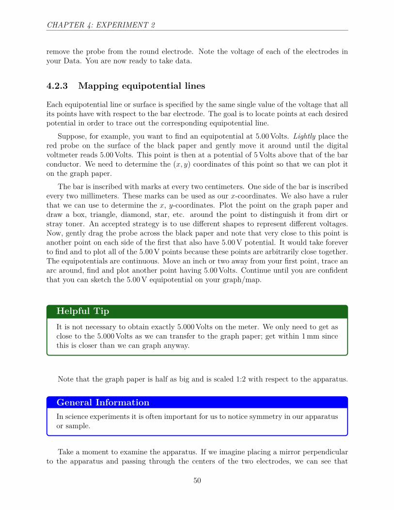
4.2.3 Mapping equipotential lines

Each equipotential line or surface is specified by the same single value of the voltage that allits points have with respect to the bar electrode. The goal is to locate points at each desiredpotential in order to trace out the corresponding equipotential line.

Suppose, for example, you want to find an equipotential at 5.00Volts. Lightly place thered probe on the surface of the black paper and gently move it around until the digitalvoltmeter reads 5.00Volts. This point is then at a potential of 5Volts above that of the barconductor. We need to determine the (x, y) coordinates of this point so that we can plot iton the graph paper.

The bar is inscribed with marks at every two centimeters. One side of the bar is inscribedevery two millimeters. These marks can be used as our x-coordinates. We also have a rulerthat we can use to determine the x, y-coordinates. Plot the point on the graph paper anddraw a box, triangle, diamond, star, etc. around the point to distinguish it from dirt orstray toner. An accepted strategy is to use different shapes to represent different voltages.Now, gently drag the probe across the black paper and note that very close to this point isanother point on each side of the first that also have 5.00V potential. It would take foreverto find and to plot all of the 5.00V points because these points are arbitrarily close together.The equipotentials are continuous. Move an inch or two away from your first point, trace anarc around, find and plot another point having 5.00Volts. Continue until you are confidentthat you can sketch the 5.00V equipotential on your graph/map.

Helpful TipIt is not necessary to obtain exactly 5.000Volts on the meter. We only need to get asclose to the 5.000Volts as we can transfer to the graph paper; get within 1mm sincethis is closer than we can graph anyway.

Note that the graph paper is half as big and is scaled 1:2 with respect to the apparatus.

General InformationIn science experiments it is often important for us to notice symmetry in our apparatusor sample.

Take a moment to examine the apparatus. If we imagine placing a mirror perpendicularto the apparatus and passing through the centers of the two electrodes, we can see that

50

CHAPTER 4: EXPERIMENT 2

the image in the mirror would be exactly the same as we see without the mirror. We callthis mirror symmetry (or bilateral symmetry) about the y-axis because of this fact. Exactlythe same stuff is at (−x, y) as is at (x, y) for all x and y. Since our apparatus has mirrorsymmetry about the y-axis, we expect that our observations will also have this symmetry.We need to test enough points to convince ourselves that our data is symmetric, but oncewe are convinced we can simply plot each point at (−x, y) and at (x, y) on the graph paperonce its coordinates are determined. If you do not observe mirror symmetry, check for loosenuts, eraser crumbs under your electrodes, or torn Teledeltos paper. Correct any problemsbefore continuing, if possible, or note any complications in your Data. Ask your teachingassistant to help you if you do not see the problem right away.

Historical AsideThe carbon paper we are using has a trade name: Teledeltos. It was developed andpatented around 1934 by Western Union. It was originally used to transmit newspaperimages over the telegraph lines (as an early fax machine). At the receiving end of the“Wirephoto”, the cylinder of a drum was covered first with a sheet of Teledeltos paper,and then with a sheet of white record paper. A pointed electrode triggered by signalstransmitted over the telegraph lines would then reconstruct the image by varying thedensity of black dots on the record paper.

Now, go after the 4Volt equipotential using the same technique. Then, do the same forthe 3Volts, 2Volts, and 1Volt equipotential lines. For each case, draw a smooth curve amongthe points having the given potential. Do not just connect the dots to get a segmented line.Remember that our measurements and plots have experimental error in them and that ourgoal is to average out these errors with a smooth data-fitting curve. The curve is intendedto fall along the equipotential between, as well as at, the specific points marked off, so thepoints should not be connected by straight line segments. Your equipotential lines shouldlook like computer fits to math models. Some data points will be above and some below,but the drawn line will be smooth compared to the data points. Label each line with itspotential. It is good strategy to trace the data points in ink and to sketch the lines in penciluntil they are satisfactory. This allows you to erase erroneous lines without erasing the data.If you erase pencil lines, please do so away from the apparatus so that the rubber (insulating)crumbs do not degrade its efficiency. Once you are satisfied with the pencil sketches, tracethe lines in ink so that the same strategy will apply to the construction of electric fieldvectors below.

4.2.4 Part 2: Finding electric field lines

Recall Equation (4.3) and apply it to an equipotential line being the path along which thecharge moves. Since all points in an equipotential have the same potential, Va = Vb forequipotentials, the work done as seen from Equation (4.4) is zero, and the work per unit

51

CHAPTER 4: EXPERIMENT 2

charge is also zero. Equation (4.3) then becomes

0 = (Va − Vb) = Wab

q=∫ b

aE · dr =

∫ b

aE · dr · cos θ (4.5)

for points a and b on the same equipotential line, surface, or volume. If the electrodes havedifferent potentials, then E 6= 0; an unbalance of charge will make an electric force and field.dr 6= 0 unless a and b are the same point; if we moved the charge, then this cannot be. Only

cos θ = 0 or θ = 90◦ remains as a possibility, but this means that the electric field, E, mustbe perpendicular to the path that we traveled, the equipotential line. Since we now have aset of equipotential lines, we can use them to sketch the electric field vectors.

CheckpointIn what way are equipotential lines oriented with respect to the electric field lines?

The result discussed earlier that the electric field is everywhere at right angles to theequipotential surfaces and the fact that electric fields start on positive charges and endon negative charges can now be used to draw the field lines in the region where you havetraced the equipotentials. On your drawing, place your pencil at a point representing thebar conductor surface and draw a line perpendicular to the bar going toward the nearestequipotential line. As your line approaches the equipotential, be sure that it curves to meetthe line at a right angle. Proceed similarly to the next equipotential, and so on until yourline ends on the drawing of the round conductor. Keep in mind that each conductor itself isan equipotential, that its surface intersects the paper in an equipotential line, and that theelectric field vector must also be perpendicular to these lines. Label the electrode’s imageswith their electric potentials. Return to the bar in the graph and construct a new linestarting at an appropriate distance (say 2 cm) from the first line. Construct 6-8 electric fieldvector lines. Place an arrow head at the end of each line to indicate the correct direction ofthe vector.

CheckpointCan you observe an electric field above and below the paper using this voltmeter?Does the electric field occupy the space above and below the paper? Why can’t thisvoltmeter observe electric fields in air? How else might these fields be observed?

4.3 Part 3: Finding electric field magnitude

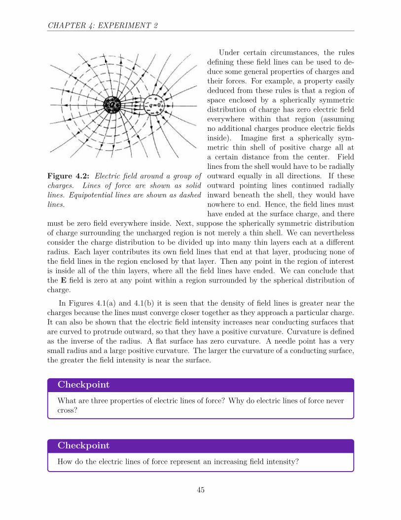
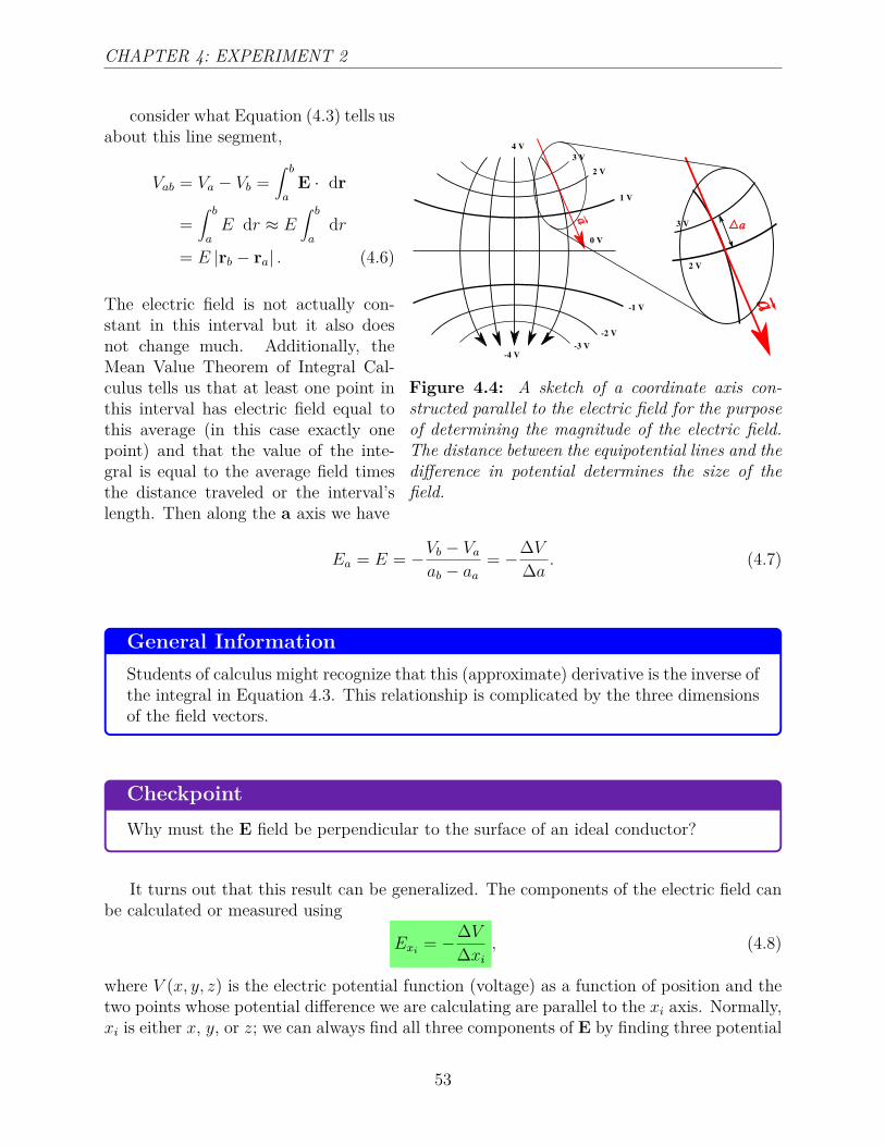
The vectors drawn above are everywhere parallel to the electric field in the paper. Since weknow the directions the E vectors point, we can imagine constructing a coordinate axis, a,parallel to a segment of one of the field vectors. Figure 4.4 illustrates this process. Let us

52

CHAPTER 4: EXPERIMENT 2

4 V

0 V

-4 V

2 V

3 V

1 V

-1 V

-2 V

-3 V

a

a

2 V

3 V a

Figure 4.4: A sketch of a coordinate axis con-structed parallel to the electric field for the purposeof determining the magnitude of the electric field.The distance between the equipotential lines and thedifference in potential determines the size of thefield.

consider what Equation (4.3) tells usabout this line segment,

Vab = Va − Vb =∫ b

aE · dr

=∫ b

aE dr ≈ E

∫ b

adr

= E |rb − ra| . (4.6)

The electric field is not actually con-stant in this interval but it also doesnot change much. Additionally, theMean Value Theorem of Integral Cal-culus tells us that at least one point inthis interval has electric field equal tothis average (in this case exactly onepoint) and that the value of the inte-gral is equal to the average field timesthe distance traveled or the interval’slength. Then along the a axis we have

Ea = E = −Vb − Vaab − aa

= −∆V∆a . (4.7)

General InformationStudents of calculus might recognize that this (approximate) derivative is the inverse ofthe integral in Equation 4.3. This relationship is complicated by the three dimensionsof the field vectors.

CheckpointWhy must the E field be perpendicular to the surface of an ideal conductor?

It turns out that this result can be generalized. The components of the electric field canbe calculated or measured using

Exi = −∆V∆xi

, (4.8)

where V (x, y, z) is the electric potential function (voltage) as a function of position and thetwo points whose potential difference we are calculating are parallel to the xi axis. Normally,xi is either x, y, or z; we can always find all three components of E by finding three potential

53

CHAPTER 4: EXPERIMENT 2

differences with one parallel to x, another parallel to y, and the last parallel to z. In thiscase, however, we have constructed our a axis parallel to E so that Ea is the only componentand E = |E| = Ea. Additionally, we have not collected potentials at points parallel to x, y,or z, so we do not have the correct information to calculate the field components. For thesegment of E between the 2V and 3V lines, the 2V point has a larger value of a. In fact,this value of a is larger than a on the 3V line by the distance between the lines. Since weknow the potentials, we can find the difference. Since we can measure the distance betweenthe lines, we can measure ∆a: ∆a is the distance between the lines. Actually, the blackpaper containing the field lines is twice as big as our map and we are measuring ∆a on ourmap. To get ∆a for the black paper, we must double our measurement. Let us supposethat we measure ∆a = 2.4 cm in Figure 4.4. Then the electric field in the black paper hasmagnitude

Ea = −∆V∆a = −2 V - 3 V

2(2.4 cm) = 0.208 V/cm. (4.9)

Actually, this is the average electric field strength along this segment of E. To get the electricfield at a point, we must repeat the experiment again and again increasing the number ofequipotential lines each time. We might imagine finding 0.1V, 0.2V,. . . , 5.9V equipotentiallines and then finding 0.01V, 0.02V,. . . , 5.99V, etc. With each repetition the lines get closertogether and the average field strength for each segment is closer to all of the points in thesegment. In calculus we call this process “taking the limit as ∆V approaches zero”. Sincethe lines get closer together as ∆V decreases, we are also “taking the limit as ∆a approacheszero”. The ratio, −∆V

∆a , gets closer and closer to some real number that is effectively thevalue of the field at the point. Symbolically, the components of the electric field at eachpoint in space are given by

Ex = − lim∆x→0

V (x+ ∆x, y, z)− V (x, y, z)∆x

Ey = − lim∆y→0

V (x, y + ∆y, z)− V (x, y, z)∆y

Ez = − lim∆z→0

V (x, y, z + ∆z)− V (x, y, z)∆z

Use Equation (4.7) as illustrated above to compute the average electric field for all sixsegments of a single field vector. Mark the vector that you use on your map so that yourreaders can verify your work. How accurately do you know ∆V and ∆a?

4.4 Analysis

Discuss the properties of the equipotential lines and the electric field vectors. Do theseobservations have the same symmetry as the apparatus that caused them? What kind ofsymmetry is this? Does the paper’s potential change when the power supply voltage ischanged? These are indications that the apparatus caused the observations.

54

CHAPTER 4: EXPERIMENT 2

Were the equipotential lines continuous as predicted? Are the field lines close together atplaces where the field magnitude is large? Are the equipotential lines more curved at placeswhere the field magnitude is large?

What subtle sources of error are present in this experiment? Are these errors large enoughto explain any discrepancies between your observations and the properties of electric fields?

4.5 Conclusions

In science a cause and its effect always have exactly the same symmetry. Can you concludethat your apparatus causes your observed equipotential lines and electric fields? Is Equa-tion (4.7) consistent with our data? If so, include this as part of your Conclusions and defineall symbols. Are you confident that this apparatus and method reveals the electric fieldaround these electrodes?

This apparatus has historical significance as a design aid. Experimenters and engineersonce constructed electrodes having a particular shape in hopes of obtaining an electric fieldsuited to a specific purpose. For example, we might need to design a vacuum tube to actas an amplifier or we might need to focus an electron beam for use in a TV’s CRT. Today,we can simply download an electrodynamics simulation program to run on our smartphone;but once upon a time the only way we could view the electric field around our electrodeswas to measure it using a similar apparatus. What other purposes can you imagine usingour apparatus to fill? Motivate interest in our work by pointing out how valuable this toolcan be for designing electric fields.

55