CHAPTER XVII: FIXING IMPROPERLY WORKING...

copyright 1997 Bruce A. McCarl and Thomas H. Spreen 1

CHAPTER XVII: FIXING IMPROPERLY WORKING MODELS ............................................ 1 17.1 Unacceptable Solution Conditions .............................................................................................................. 1

17.1.1 Solver Failure -- Causes and Prevention ............................................................................................. 1 17.1.2 Unbounded or Infeasible Solutions ...................................................................................................... 2 17.1.3 Unsatisfactory Optimal Solutions ......................................................................................................... 2

17.2 Techniques for Diagnosing Improper Models ........................................................................................... 3 17.2.1 Simple Structural Checking ................................................................................................................... 3

17.2.1.1 Analytical Checking ........................................................................................................................ 3 17.2.1.2 Numerical Model Analysis ............................................................................................................ 4

17.2.2 A Priori Degeneracy Resolution ........................................................................................................... 5 17.2.3 Altering Units of Constraints and Variables: Scaling ........................................................................ 5

17.2.3.1 Scaling-The Basic Procedure ......................................................................................................... 6 17.2.3.2 Mathematical Investigation of Scaling ......................................................................................... 8

17.2.3.2.1 Variable Scaling ....................................................................................................................... 9 17.2.3.2.2 Effects of Constraint Scaling ................................................................................................ 12 17.2.3.2.3 Objective Function and Right Hand Side Scaling ............................................................. 13

17.2.3.4 Summary ......................................................................................................................................... 14 17.2.3.5 Empirical Example of Scaling ..................................................................................................... 15

17.2.4 The Use of Artificial Variables to Diagnose Infeasibility .............................................................. 17 17.2.5 Use Unrealistically Large Upper Bounds to Find Causes of Unboundedness ............................. 19 17.2.6 Budgeting ............................................................................................................................................... 21 17.2.7 Row Summing ....................................................................................................................................... 24

References .............................................................................................................................................................. 26

copyright 1997 Bruce A. McCarl and Thomas H. Spreen

1

CHAPTER XVII: FIXING IMPROPERLY WORKING MODELS

Empirical models do not always yield acceptable solutions. This chapter contains discussion of

unacceptable solution conditions and techniques for diagnosing the causes of such conditions.

17.1 Unacceptable Solution Conditions

Four cases of improper solutions can arise. First, a solver could fail exhibiting: a) a time, iteration,

or resource limit; b) a lack of meaningful progress; or c) a report of numerical difficulties. Second, a solver

may halt identifying that the problem is infeasible. Third, a solver may halt identifying that the problem is

unbounded. Fourth, the solver may yield an "optimal," but unacceptable solution.

17.1.1 Solver Failure -- Causes and Prevention

When solvers fail because of numerical difficulties or use an unrealistically large amount of

resources to make little progress, the modeler is often in an awkward position. However, several actions

may alleviate the situation.

One should first examine whether the model specification is proper. The section on structural

checking below gives some techniques for examining model structure. In addition traditional input

(commonly called MPS input) based solvers frequently fail because of improper coefficient location

(although GAMS prevents some of these errors). In particular, errors can arise in MPS coefficient

placement or item naming resulting in more than one (duplicate) coefficient being defined for a single

matrix location. Given our concentration on the GAMS modeling system, procedures for finding duplicate

coefficients will not be discussed. Nevertheless, this is probably the most common reason why MPS input

based solvers run out of time.

The second reason for solver failure involves degeneracy induced cycling. Apparently, even the

best solvers can become stuck or iterate excessively in the presence of massive degeneracy. Our

experience with such cases indicates one should use an a priori degeneracy resolution scheme as discussed

below. We have always observed reduced solution times with this modification.


2

Thirdly, a solver may fail citing numerical difficulties, an ill-conditioned basis or a lack of

progress. Such events can be caused by model specification errors or more commonly poor scaling. Often

one needs to rescale the model to narrow the disparity between the magnitude of the coefficients. Scaling

techniques are discussed below.

All of the preventative techniques for avoiding solver failures can be used before solving a model.

Modelers should check structure and consider scaling before attempting model solutions. However,

degeneracy resolution should not usually be employed until a problem is identified.

17.1.2 Unbounded or Infeasible Solutions

Often the applied modeler finds the solver has stopped, indicating that the model is infeasible or

unbounded. This situation, often marks the beginning of a difficult exercise directed toward finding the

cause of the infeasibility or unboundedness, particularly when dealing with large models. There are several

techniques one can use when this occurs. The first involves structural checking to find obvious model

formulation defects. The second and third techniques involve the use of artificial variables and large upper

bounds to find difficulties. Finally one could use the techniques called budgeting and row summing.

17.1.3 Unsatisfactory Optimal Solutions

Unfortunately, optimal solutions can be unrealistic. Discovering an optimal solution means the

problem has a mathematically consistent optimum. However, mathematical consistency does not

necessarily imply real world consistency (Heady and Candler). Usually, unrealistic solutions may be

caused by improper problem specification or assumption violations. Cases arise where the model solution

is improper because of: a) omitted constraints or variables; b) errors in coefficient estimation; c) algebraic

errors; or d) coefficient placement errors.

Basically, a model may be judged improper because of incorrect valuation or allocation results.

Valuation difficulties arise from the reduced cost or shadow price information, such items take on values

when primal reduced costs are formed. Allocation difficulties arise when the slack or decision variable

values are unrealistic. The values of these items are formed through the constraint interactions. Thus, to


3

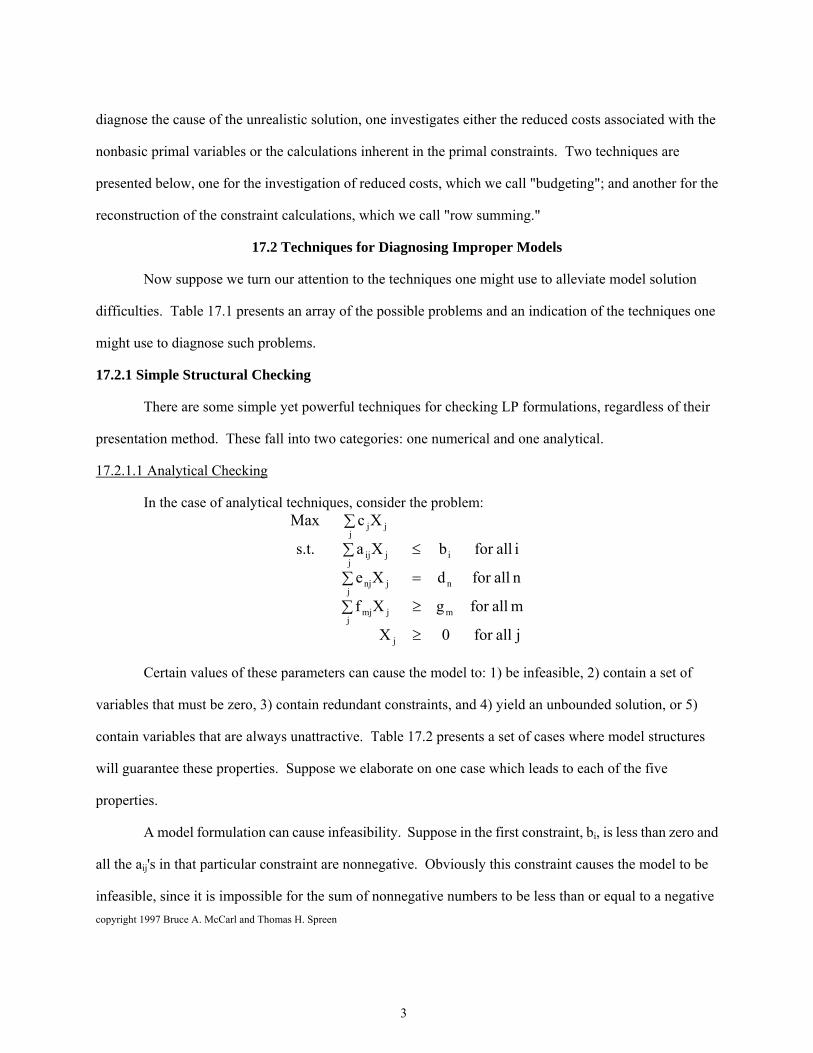
diagnose the cause of the unrealistic solution, one investigates either the reduced costs associated with the

nonbasic primal variables or the calculations inherent in the primal constraints. Two techniques are

presented below, one for the investigation of reduced costs, which we call "budgeting"; and another for the

reconstruction of the constraint calculations, which we call "row summing."

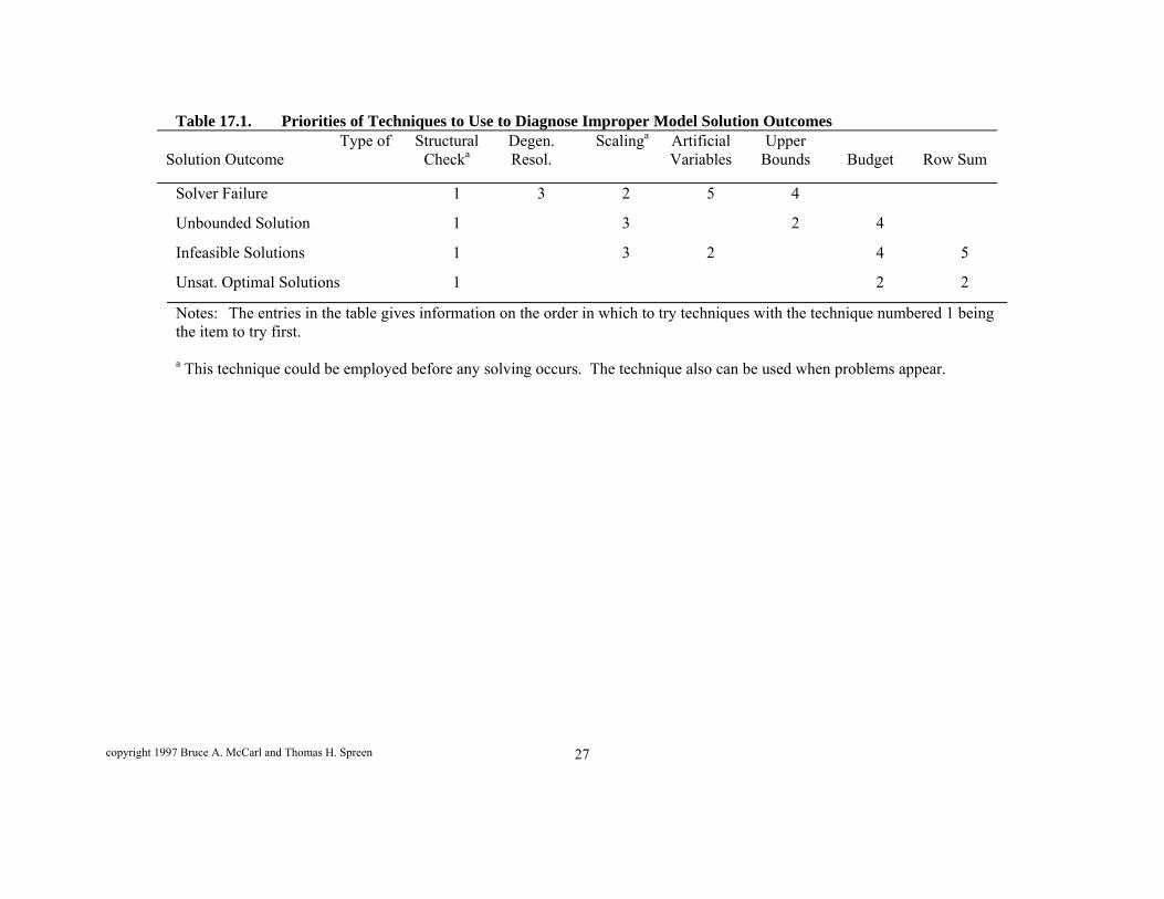
17.2 Techniques for Diagnosing Improper Models

Now suppose we turn our attention to the techniques one might use to alleviate model solution

difficulties. Table 17.1 presents an array of the possible problems and an indication of the techniques one

might use to diagnose such problems.

17.2.1 Simple Structural Checking

There are some simple yet powerful techniques for checking LP formulations, regardless of their

presentation method. These fall into two categories: one numerical and one analytical.

17.2.1.1 Analytical Checking

In the case of analytical techniques, consider the problem:

j allfor 0X

m allfor gXf

n allfor dXe

i allfor bXas.t.

XcMax

j

mj

jmj

nj

jnj

ij

jij

jjj

Certain values of these parameters can cause the model to: 1) be infeasible, 2) contain a set of

variables that must be zero, 3) contain redundant constraints, and 4) yield an unbounded solution, or 5)

contain variables that are always unattractive. Table 17.2 presents a set of cases where model structures

will guarantee these properties. Suppose we elaborate on one case which leads to each of the five

properties.

A model formulation can cause infeasibility. Suppose in the first constraint, bi, is less than zero and

all the aij's in that particular constraint are nonnegative. Obviously this constraint causes the model to be

infeasible, since it is impossible for the sum of nonnegative numbers to be less than or equal to a negative


4

number.

Second, it is possible that the constraints require that certain variables be zero. Consider what

happens if in the second constraint the right hand side (dn) equals to zero and all enj's are greater than or

equal to zero, then every variable with a nonzero coefficient in that constraint must be zero.

There are also cases where the model possesses redundant constraints. Suppose bi is positive, but

all aij's are negative or zero; then, clearly, this constraint will be redundant as the sum of negative numbers

will always be less than or equal to a positive number.

Checks can also be made for whether the problem is unbounded or contains variables which will

never come into the solution. Consider an activity with a positive objective function coefficient which has

all nonzero aij's negative, all zero enj's and all nonzero fmj's positive. Clearly, then, this variable contributes

revenue but relaxes all constraints. This will be unbounded regardless of the numerical values. Further,

variables may be specified which will never come into the solution. For example, this is true when cj is less

than 0, all nonzero aij's are greater than 0, enj's zero, and nonzero fmj's negative.

These particular structural checks allow one to examine the algebraic formulation or its numerical

counterpart. Unfortunately, it is not possible to make simple statements when the constraint coefficients are

of mixed sign. In such cases, one will have to resort to numerical checking. All of the procedures above

have been automated in GAMSCHCK although they can be programmed in GAMS (See McCarl, 1977).

17.2.1.2 Numerical Model Analysis

Another model analysis methodology involves numerical investigation of the equations and

variables. Here, one prints out the equations of a model (in GAMS by using the OPTION LIMROW and

LIMCOL command) and mentally fixes variables at certain levels, and then examines the relationship of

these variables with other variables by examining the equations. Examples of this are given in the joint

products problem above. Numerical model analysis can also be carried out by making sure that units are

proper, using the homogeneity of units tests.

Another numerical technique involves use of a "PICTURE" with which coefficient placement and


5

signs can be checked. GAMS does not contain PICTURE facilities, so we do not discuss the topic here,

although one is contained in GAMSCHK (see McCarl, 1977).

17.2.2 A Priori Degeneracy Resolution

Degeneracy can cause solvers to cycle endlessly making little or no progress. Solvers like MINOS

( Murtaugh and Saunders, 1983) on occasion give messages like "terminating since no progress made in last

1000 iterations" or "Sorry fellows we seem to be stuck." Our experience with such cases indicates one

should use an a priori degeneracy resolution scheme adding small numbers to the right hand sides,

especially to those constraints which start out with zero or identical right hand sides. The magnitude of the

small numbers should be specified so that they are not the same for all rows and so that they do not

materially affect the solution. Thus, they might be random or systematically chosen numbers of the order

10-3 or 10-4 (although they can be larger or smaller depending on the scaling and purpose of the constraints

as in McCarl, 1977). We have always observed reduced solution times with this modification. OSL

automatically invokes such a procedure.

17.2.3 Altering Units of Constraints and Variables: Scaling

Scaling is done automatically in a number of algorithms including MINOS which is used in

GAMS. However, automatic scaling is not always successful. Modelers are virtually always more

effective in scaling (Orchard-Hayes). This section explores scaling procedures, discussing the effects on

resulting optimal solutions.

Altering the units of constraints and variables improves the numerical accuracy of computer

algorithms and can reduce solution time. Scaling is needed when the disparity of matrix coefficient

magnitudes is large. An appropriate rule of thumb is, one should scale when the matrix coefficient

magnitudes differ in magnitude by more than 103 or 104. In other words, scaling is needed if the aij coeffi-

cient with the largest absolute value divided by the coefficient with the smallest nonzero absolute value

exceeds 10000. One achieves scaling by altering the formulation so as to convert: a) the objective function

to aggregate units (i.e., thousands of dollars rather than dollars), b) constraints to thousands of units rather


6

than units (i.e., one might alter a row from pounds to tons), or c) variables into thousands of units (e.g.,

transport of tons rather than pounds).

17.2.3.1 Scaling-The Basic Procedure

Given the LP problem

0X ,X

bXaXa

bXaXas.t.

XcXcMax

21

2222121

1212111

2211

Suppose one wished to change the units of a variable (for example, from pounds to thousand

pounds). The homogeneity of units test requires like denominators in a column. This implies every

coefficient under that variable needs to be multiplied by a scaling factor which equals the number of old

variable units in the new unit; i.e., if Xj is in old units and X'j is to be in a new unit, with aij and a'ij being the

associated units.

Xj' = Xj/ SCj;

where SCj equals the scaling coefficient giving the new units over the old units

aij' = aij / (SCj).

The scaling procedure can be demonstrated by multiplying and dividing each entry associated with the

variable by the scaling factor. Suppose we scale X1 using SC1

0 X X

b XaSC / X a SC

b XaSC / X a SCs.t.

XcSC / X c SCMax

21

222211211

121211111

221111

or substituting a new variable X1' = X1/SC1 we get

0 X X

b XaX a SC

b XaX a SCs.t.

XcX c SCMax

21

2222'1211

1212'1111

22'111

Variable scaling alters the magnitude of the solution values for the variables and their reduced cost as we


7

will prove later.

Scaling can also be done on the constraints. When scaling constraints; e.g., transforming their units

from hours to thousands of hours, every constraint coefficient is divided by the scaling factor (SR)

as follows:

0 X ,X

b Xa Xa

SR / b X SR / aX SR / a

Xc Xc Max

21

2222121

1212111

2211

where SR is the number of old units in a new unit and must be positive. Constraint scaling affects :1) the

slack variable solution value, which is divided by the scaling factor; 2) the reduced cost for that

slack, which is multiplied by the scaling factor; and 3) the shadow price, which is multiplied by the scaling

factor.

The way scaling factors are utilized may be motivated by reference to the homogeneity of units

section. The coefficients associated with any variable are homogeneous in terms of their denominator

units. Thus, when a variable is scaled, one multiplies all coefficients by a scaling factor (the old unit over

the new unit) changing the denominator of the associated coefficients. Constraints, however, possess

homogeneity of numerator units so, in scaling, we divide through by the new unit divided by the old unit.

Thus, when changing a constraint from pounds to tons one divides through by 2000 (lbs/tons).

Two other types of scaling are also relevant in LP problems. Suppose that the right hand sides are

scaled, i.e., scaled from single units of resources available to thousands of units of resources available.

Then one would modify the model as follows:

0X ,X

SH / bXaXa

SH / bXaXas.t.

XcXcMax

21

2222121

1212111

2211

The net effects of this alteration will be that the optimal value of every decision variable and slack would be


8

divided by the scaling factor, as would the optimal objective function value. The shadow prices and

reduced costs would be unchanged.

One may also scale the objective function coefficients by dividing every objective function

coefficient through by a uniform constant (SO).

0X ,X

bXa Xa

bXa X a

X SO / cX SO / cMax

21

2222121

1212111

2211

Under these circumstances, the optimal decision variables and slack solutions will be unchanged;

but both the shadow prices and reduced costs will be divided by the objective function scaling factor as will

be the optimal objective function value.

Scaling may be done in GAMS using an undocumented feature. Namely putting in the statement

variablename.scale = 1000 would cause all variables in the named variable block to be scaled by 1000 with

the solution automatically being readjusted. Similarly equationname.scale = 1000 will scale all constraints

in a block. This must be coupled with the command Modelname.scaleopt=1.

17.2.3.2 Mathematical Investigation of Scaling

In this section an investigation will be carried out on the effects of scaling using the matrix algebra

optimality conditions for a linear program. Readers not interested in such rigor may wish to skip to the

summary and empirical example.

The optimality conditions for the LP problem are given by

CB B-1 aj - cj ≤ 0 for all j

B-1 b ≤ 0.

Given such a solution the optimal decision variables are given by

XB = B-1 b,

the shadow prices by


9

U = CB B-1

and the reduced costs by

CB B-1 aj - cj,

and the optimal Z value is

Z = CB B-1 b

In our investigation, we examine the impact of scaling on each of these items.

17.2.3.2.1 Variable Scaling

When a variable is scaled, the problem becomes:

0 X X

b XaX a SC

b XaX a SCs.t.

XcX c SCMax

21

2222'1211

1212'1111

22'111

where X1 equals SCX'1 and SC is a positive scalar.

The effect on the solution depends on whether the scaled variable is basic or nonbasic. First,

consider nonbasic variables. If a nonbasic variable is scaled, then the scaling operation does not affect the

basis inverse. Thus, the only thing that needs to be investigated is whether or not scaling the nonbasic

variable renders it attractive to bring into the basis. This involves an investigation of the reduced cost after

scaling. Constructing the reduced cost for this particular variable

CB B-1 SC aj - SC cj = SC (CB B-1 aj - cj)

we find that the reduced cost after scaling (new) equals the reduced cost before scaling (old) times the

scaling factor. Thus, we have the old reduced cost multiplied by the scaling constant and under positive SC

the before scaling solution remains optimal. The only alteration introduced by scaling a nonbasic variable

is that its reduced cost is multiplied by the scaling factor. This can be motivated practically. If it costs $50

to enter one acre of a crop not being grown into solution, it would logically cost $50,000 to bring in a

thousand acres of that crop.

Now suppose a basic variable is scaled. In this case, the basis inverse is altered. Suppose that the


10

basis matrix before scaling is B, while the matrix of technical coefficients before scaling is A. The new

matrices (B*,A*) can be expressed as the old matrices (B,A) post-multiplied by matrices KA and KB which

are modified identity matrices. Assuming the nth column of B is being scaled, then the element on the

diagonal in the nth column of the KB matrix will be the scaling factor. Thus,

A* = AKA B* = BKB

where

1...0...000

.....................

0...SC...000

.....................

0...0...100

0...0...010

0...0...001

K B

The KA matrix would be formed similarly with the column in the A matrix being scaled identifying the

diagonal element where SC appears.

We may derive a relationship between the basis inverses before and after scaling. Matrix algebra

theory shows that

(B*)-1 = (BKB)-1 = KB-1 B-1

We should also note that the scaled objective function coefficients of the basic variables are post-multiplied

by KB, i.e.,

CB = CB KB

Now let us look at the optimality criteria for non-basic variables

.c - a B C *j

*j

1-**B

The reduced cost after scaling becomes

0 c - a BC

c - a KKCc - a BC

jj1-

B

jj-1BBB

*j

*j

1-**B


11

since KBK-1 = I. Thus, the reduced costs after scaling equal the reduced costs before scaling. Thus, we have

proven that the solution will remain optimal.

We now need to turn our attention to whether or not the basic variables remain nonnegative. The

values of the basic variables at optimality are given by B*-1b. Substituting in our relationships, we obtain

.X K b B K b B X B-1B

-1-1B

1-**B

The scaled solution equals KB-1 times the unscaled solution. The inverse of KB is an identity-like

matrix with one over the scaling factor on the diagonal in the position where the scaled variable enters the

basis.

1...0...000

.....................

0...1/SC...000

.....................

0...0...100

0...0...010

0...0...001

K 1-B

The KB -1 XB multiplication yields the vector

mB

KB

2B

1B

B1-BB

X

...

SC / X

...

X

X

XKX

Thus, scaling reduces the magnitude of the particular basic variable being scaled, while all other variables

are unaffected.

We may also investigate the objective function consequences. The optimal objective function

value of the scaled problem is

Z bBC bBKK C bBC Z -1B

1-*-1BB

*B

1-**B

*

Clearly, then, the objective function value after the change equals the objective function value before the


12

change. All in all, column scaling leaves the problem with the same qualitative answer. The solution value

of the particular variable being scaled and its reduced cost are altered by the scaling factor.

17.2.3.2.2 Effects of Constraint Scaling

When one scales a constraint, the resultant problem appears as

0X ,X

bXa Xa

SR / bX SR / aX SR / a

Xc Xc Max

21

2222121

1212111

2211

or

,

0X 0X

bXAs.t.orRbRAXs.t.

CXMaxCXMax**

where R is a scaling matrix of the form

1...0...000

.....................

0...1/RS...000

.....................

0...0...100

0...0...010

0...0...001

R

Further, the new basis (B*) is related to the old basis as follows

B* = RB

and the basis inverse is the old basis inverse multiplied by the inverse of R.

B*-1 = B-1 R-1

Again, R-1 is an identity-like matrix quality.


1...0...000

.....................

0...RS...000

.....................

0...0...100

0...0...010

0...0...001

R 1-

Now let us turn our attention to the effects of scaling a constraint. We will derive the results

assuming the slack variable is not in the basis. The reduced cost criteria for the scaled problem is given by

jj-1

Bjj-1-1

B*j

*j

1-**B c - aBC c - Ra R BC c - a BC

Thus, the optimality conditions are the same as before scaling and the solution remains optimal with

unchanged reduced costs. We now may investigate the variable solution values. For the scaled problem, the

solution values are

X*B = B*-1 b* = B-1 R-1 R b = B-1 b

which shows that the values of the basic variables are unaffected. The objective function is also unchanged.

Thus, the optimality and feasibility of the basis remain entirely unaffected. What then does change?

The shadow prices after scaling are

U = CB B-1 R-1.

Given the form of R-1 from above, the shadow prices are identical to the shadow prices before scaling

Ui = (CB B-1)i

for all rows but the particular row being scaled. For that row, the shadow price is multiplied by the

scaling factor

Ui = (CB B-1)i RS

Finally we should note that when a slack variable is in the basis, then constraint scaling simply

changes the magnitude of the optimal slack variable value by dividing it by the scaling factor.

17.2.3.2.3 Objective Function and Right Hand Side Scaling

If the objective function coefficients are uniformly divided by a constant, the values of the solution


variables (B-1 b) are unaffected. However, the magnitudes of the shadow prices (CB B-1), the optimal

objective function value (CB B-1b), and the reduced costs (CB B-1aj - cj) are affected. In all of these cases,

these items would be uniformly divided by the objective function scaling factor. A similar observation can

be made regarding scaling the right hand side. The right hand side determines only the objective function

value (CB B-1 b) and the solution value of the basic variables (B-1 b). Dividing all right hand sides by a

constant would divide the objective function and all the optimal variable values by the same constant.

17.2.3.4 Summary

Scaling alters coefficient magnitudes within the matrix and the resultant magnitude of selected

items in the solution. Consider the LP problem

0X

bAXs.t.

CXMax

Suppose a set of positive (all scaling factors must be positive) scaling factors will be applied to the LP

model. The scaling factors are a) COLSCALj for the jth variable - a factor multiplying every coefficient

under that variable, b) ROWSCALi for the ith constraint - a factor dividing every coefficient in that

constraint, c) OBJSCAL for the objective function - a factor dividing every coefficient in the objective row

and d) RHSSCAL for the right hand side - a factor dividing every right hand side value. The parameters of

the model after scaling are:

RHSSCAL *ROWSCAL

1*bb

ROWSCAL

COLSCAL*aa

OBJSCAL

COLSAL*cc

ii

'i

i

jij

'ij

jj

'j

where the / denotes the new coefficients. The relationship between solution items before and after scaling is

given in Table 17.3. Thus, if a particular variable j is scaled by 1000 and constraint i is scaled by a 1000, the

aij value is numerically unchanged. However, if variable j is scaled by 1000 and constraint i was scaled by

100, then the value of the aij coefficient is multiplied by 10.

Thus, for example, if an optimal variable value before scaling was 6 and the right hand side is


multiplied by 100 while the coefficients of that variable are multiplied by .02 then the resultant value after

scaling would be 3.

Finally, we must emphasize that the only proper way of scaling is to operate on all coefficients for

each variable, right hand side and objective function in the same manner. One cannot selectively scale

selected coefficients. The interaction of the various scaling factors can make it look like one is only scaling

selected coefficients, as will be demonstrated in the empirical example below. But this is not the case,

consistency must be maintained.

17.2.3.5 Empirical Example of Scaling

The previous discussion deals with the implications of changes in constraint, variable, right hand

side and objective function units. The reader, however, should note that gains in terms of numerical stability

may arise only when several items are simultaneously scaled. This is illustrated in the example. Consider

the following problem

0XXXX

3000045X50X

6000002000X1500X

050X -4X 5X

08000X-10000X- Xs.t.

500X-400X -X500 XMax

4321

32

32

432

321

4321

where:

X1 is the sale of nibbles in pounds. It returns $1 of profit per unit and removes one pound

from the nibble balance row.

X2 is the hours of nibble production via process 1. One hour's worth of production uses $500

worth of direct cost, 5 units of gribbles, 1500 hibbles and 50 hours of labor. As a result,

one gets 10,000 nibbles.

X3 is the hours of nibble production using process 2 . Here 8000 nibbles are produced at a

direct cost of $400 with four pounds of gribbles used, 2,000 hibbles, and 45 hours of labor

produced.

X4 is the number of 50 pound sacks of gribbles purchased, costing $5000 and providing 50

pounds of gribbles into the gribble balance row.


The right hand side shows an endowment of 600,000 hibbles and 30,000 hours of labor. The objective

function is in the units of dollars and represents profit. The first constraint balances the units of nibbles

produced with those sold. The second constraint balances the units of gribbles used with those purchased.

The third constraint limits the number of hibbles used to the fixed endowment. The fourth

constraint limits the hours of labor used to the fixed endowment. Non-negativity of all variables is assumed.

This problem is not well-scaled and its scaling characteristics will be altered. (This will be done to

illustrate scaling - the problem is scaled satisfactorily for any solver). At solution, the objective function

equals 3,600,000 and the variables values (with their units) are shown in Table 17.4.

Now suppose we scale the first constraint by dividing through by 1000. Simultaneously, let us

scale the third constraint by dividing through by 100, and divide the fourth constraint by 10. This changes

the units of these constraints such that the first constraint is in thousands of nibbles, the third constraint is

hundreds of hibbles, and the fourth constraint is in 10's of labor hours. The new model resulting from the

scaling is

0X,XXX

30004.5X5X

600020X15X

0X 4X 5X

08X -10X -X

100X-400X-500X-1000XMax

4321

32

32

432

321

4321

According to Table 17.3 the optimal shadow price on constraint 1 will be the corresponding

prescaled solution value multiplied by 1,000, the shadow price on constraint 3 is multiplied by 100 and the

shadow price for constraint 4 is increased by a factor of 10. The primal solution variables are unchanged as

well as the value of the objective function. The solution to this model is shown in Table 17.5. The impact

of scaling on the optimal solution is as forecast.

The optimal objective function value equals 1.8 million. Note, we really have not gained anything

with scaling as there is the same disparity of orders of magnitudes within the matrix as before. Further

scaling will alter this. Suppose we choose to rescale X1 into 1000's of pounds and X4 to pounds. This

involves multiplying all coefficients in the X1 column by 1000 and all coefficients associated with X4 by

.02.


The formulation subsequent to this scaling is

0X,X,X,X

30004.5X5X

600020X15X

0X-4X5X

08X-10X-Xs.t.

100X-400X-500X-1000XMax

4321

32

32

432

321

4321

The net effect of this scaling operation causes the optimal solution X1 value to be divided by 1000, and X4 to

be divided by .02. The resultant solution is shown in Table 17.6.

The solution again corresponds to predictions. The optimal value of the objective function equals

1.8 million. This particular problem is now fairly well scaled; however, for illustrative purposes suppose

that we scale the objective function and right hand side. First, suppose we divide the objective function by

1000 and the right hand side coefficients by 100. The resulting LP problem is

0X,X,X,X

304.5X5X

6020X15X

0X-4X5X

08X-10X-Xs.t.

0.1X-0.4X-0.5X-XMax

4321

32

32

432

321

4321

This should result in a solution with the shadow prices and reduced costs divided through by 1000, the objective

function by 100,000 and the variable solution values by 100. The optimal solution is shown in Table 17.7. The

optimal value of the objective function equals 18. This solution can easily be shown to

be equivalent to the solution of the unscaled problem, Table 17.4, through the scaling relations in

Table 17.3.

Summarizing, scaling allows one to narrow the discrepancies within the magnitudes of the

numbers within the matrix. One can, given the scaling factors, derive the original unscaled

solution from the scaled solution. Practitioners should use scaling to decrease disparities in order

of magnitude which will severally improve the performance of the solution algorithm.

17.2.4 The Use of Artificial Variables to Diagnose Infeasibility

Often the applied modeler finds the solver has stopped indicating that the model is infeasible. This


situation, particularly when dealing with large models, often marks the beginning of a difficult exercise.

There are several ways one can proceed. The first technique involves use of the above simple structural

checking procedures to insure that the rows with minimum requirements have some way of satisfying those

minimum requirements. Also, if available, a "picture" also can be used to find misplaced coefficients,

misspecified or duplicate coefficients. However, suppose that all the simple mechanical checks are

examined and the model is still infeasible or unbounded, then what?

There is an empirical approach involving the use of artificial variables. As discussed in Chapter 2,

artificial variables permit infeasible solutions to appear feasible. Artificial variables have a large negative

objective function coefficient (when the objective is to maximize) and positive in a single constraint.

Artificial variables only remain in the solution when the restrictions with which they are associated cannot

be met, as occurs in misspecified LP models. For example, a model might contain a minimum requirement

of 10,000 units production whereas the labor resource availability constraint permits fewer units. This

problem may arise if: a) the 10,000 unit requirement is too large and has been improperly entered, b) the

labor endowment is erroneously too small, c) the labor requirements for production have been

overestimated, or d) the contribution to the minimum requirement constraint is too small.

The last three cases arise when the minimum requirement level is correct, but the infeasibility is

caused by misspecifications in other coefficients. Thus, infeasibilities arise not only because of improperly

specified minimum requirement rows, but also because of errors in other coefficients.

The question is "how can one discover the cause of the infeasibility?" This can be done by adding

artificial variables to the model formulation. The inclusion of artificial variables permits all models to have

feasible optimal solutions regardless of whether the "real" constraints are satisfied. Infeasible solutions

exhibit nonzero artificial variables. Nonzero artificial variables will cause a large negative objective

function value and large shadow prices since some CB's in the CB B-1 computations are large. Specifically,

constraints which exhibit large shadow prices are those involved with the infeasibility. The constraints not

causing the infeasibility will have unaffected shadow prices. Thus, the imposition of artificial variables

allows one to identify which constraints are nominally causing the infeasibility. We do not argue that such

information cannot be found in an ordinary infeasible solution; however, it is more difficult to interpret.


Ordinarily, infeasible solver solutions are detected by phase 1 of the simplex algorithm wherein the shadow

prices give the marginal contribution of a change in the right hand side to the sum of the infeasibilities.

To illustrate the use of artificial variables in the context of an infeasible model consider the

following example:

0X,X

20X

65X50X

50XX s.t.

50X50XMax

21

1

21

21

21

This problem is infeasible due to the interaction of the second and third constraints. Suppose that an error

was made and the number 50 which is specified as the requirement of X1 for the second resource should

have been 0.50. The third constraint has a minimum requirement, thus an artificial variable is included.

20A X

65X50X

50XX

10000A-50X50XMax

1

21

21

21

Here the artificial variable A is entered with a large negative number in the objective function and a

plus one in the third constraint, thus permitting a minimum requirement to be satisfied. The solution to the

augmented problem is shown in Table 17.8. The value of the objective function is -186,935. In this

solution, the artificial variable A is nonzero with the second and third constraints binding. The shadow

prices on the second and third constraints reflect the influence of the artificial variable. Thus, the modeler

would receive signals that there was something wrong in the interaction of the second and third constraints.

Hopefully then the data error would be found.

In summary, artificial variables are useful in finding the source of infeasibility. Artificials are only

needed in constraints that are not satisfied when the decision variables are zero. Their use allows the model

user to find infeasibilities by narrowing attention to the constraints which are the underlying causes of the

infeasible solution. We also feel they should be used where infeasibilities can arise in models which: a)

continually have their data altered; and b) are used by people other than the modeler (see McCarl et al.).

17.2.5 Use Unrealistically Large Upper Bounds to Find Causes of Unboundedness


LP problems may also yield unbounded solutions. One can again use structural checking or a

picture to find the problem. However, if these checks fail, imposition of large upper bounds in an

unbounded model on all variables which exhibit desirable objective function coefficients will prevent

unboundedness, and will cause the variables causing unboundedness to take on large solution values.

Investigation of the variables which take on such large values will allow the modeler to find the cause of the

unboundedness. Consider a LP problem which has large upper bounds imposed.

0X

MX

bAXs.t.

cXMax

Here the equations X ≤ M are upper bound constraints limiting the decision variables to a large number

(e.g., the constraint X1 ≤ 100,000 has been imposed on the model). Given decision variables, M would be

set so it was unrealistically large (i.e., 1,000 times larger than the largest expected X value). Why would

anyone want to impose such bounds? Consider the following simple example.

0X,X,X

5X

0X-X

XX-3XMax

321

3

21

321

This problem is unbounded: the model can purchase X2, using it to produce X1 at a net operating profit of $2

without limit. However, the imposition of the constraint X1 ≤ 100,000 yields the solution X1 = X2 =

100,000, X3 = 50. Thus, if the model user saw this solution and felt that X1 = 100,000 was unrealistically

large then this would show that there is something wrong within the model. It also shows that X1 and X2 are

the items involved with the unboundedness while X3 is not a factor.

The use of large upper bounds precludes the possibility of an unbounded solution but causes the

objective function and some of the variables to take on unrealistically large values. Subsequently, one can

trace the cause of the unboundedness by examining the set of variables which are unrealistically large. This

is important since ordinarily LP solvers are implemented so that when they discover an unbounded solution

they automatically stop. This leaves the user without much information as to the cause of the


unboundedness.

Decision modelers may wish to upper bound the sum of a number of variables rather than each and

every variable. This could be done by using the following:

j allfor 0X

MX

i allfor bXas.t.

XcMax

j

jj

ij

jij

jjj

Here one specifies that the sum of all variables is less than or equal to an unrealistically large number.

17.2.6 Budgeting

Yet another model analysis technique, particularity when dealing with unrealistic optimal

solutions, involves Budgeting. Budgeting herein refers to the reconstruction and examination of reduced

cost and shadow price information. The procedure is best illustrated through example. Consider the model

shown in Table 17.9.

This model contains activities for buying miscellaneous inputs; selling corn, soybeans, and pork;

and producing corn, soybeans, and hogs. The model is maximized subject to a resource constraint on land,

along with supply-demand balances on pork, soybeans, corn, and miscellaneous inputs. The miscellaneous

input item is specified in dollars and therefore enters the objective function at a per unit cost of $1 while

supplying a dollar's worth of miscellaneous inputs. Corn is sold for $2.50 per unit, soybeans $6 per unit,

and pork $.50 per unit. Corn production incurs $75 in direct production costs and $125 in miscellaneous

inputs while using one acre of land and yielding 120 bushels of corn. Soybean production costs $50 in

direct production costs and another $50 in miscellaneous inputs while using an acre of land and yielding 50

bushels of soybeans. Hog production has no direct costs, uses $20 in miscellaneous inputs, and requires 20

bushels of corn. An unrealistically large yield in the hog activity has been entered (1000 pounds per hog).

This example "error" will be sought by the budgeting technique.

The optimum solution to this model is shown in Table 17.10. The optimal value of the objective

function is $1,508,000. This solution includes several symptoms that there is something wrong. For

example, 3,600,000 pounds of pork are sold, the reduced cost on raising soybeans is $2,480 an acre, the

shadow price on land is $2,680 and the shadow price of corn is $24 a bushel. Budgeting investigates the


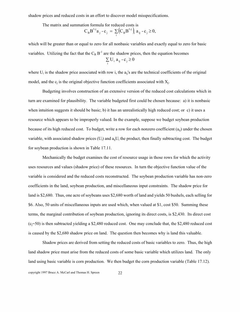
shadow prices and reduced costs in an effort to discover model misspecifications.

The matrix and summation formula for reduced costs is

i

jiji1-*

Bjj1-*

B 0, c - a BC c - aBC

which will be greater than or equal to zero for all nonbasic variables and exactly equal to zero for basic

variables. Utilizing the fact that the CB B-1 are the shadow prices, then the equation becomes

i

jiji 0 c - a U

where Ui is the shadow price associated with row i, the aij's are the technical coefficients of the original

model, and the cj is the original objective function coefficients associated with Xj.

Budgeting involves construction of an extensive version of the reduced cost calculations which in

turn are examined for plausibility. The variable budgeted first could be chosen because: a) it is nonbasic

when intuition suggests it should be basic; b) it has an unrealistically high reduced cost; or c) it uses a

resource which appears to be improperly valued. In the example, suppose we budget soybean production

because of its high reduced cost. To budget, write a row for each nonzero coefficient (aij) under the chosen

variable, with associated shadow prices (Ui) and aijUi the product, then finally subtracting cost. The budget

for soybean production is shown in Table 17.11.

Mechanically the budget examines the cost of resource usage in those rows for which the activity

uses resources and values (shadow price) of these resources. In turn the objective function value of the

variable is considered and the reduced costs reconstructed. The soybean production variable has non-zero

coefficients in the land, soybean production, and miscellaneous input constraints. The shadow price for

land is $2,680. Thus, one acre of soybeans uses $2,680 worth of land and yields 50 bushels, each selling for

$6. Also, 50 units of miscellaneous inputs are used which, when valued at $1, cost $50. Summing these

terms, the marginal contribution of soybean production, ignoring its direct costs, is $2,430. Its direct cost

(cj=50) is then subtracted yielding a $2,480 reduced cost. One may conclude that, the $2,480 reduced cost

is caused by the $2,680 shadow price on land. The question then becomes why is land this valuable.

Shadow prices are derived from setting the reduced costs of basic variables to zero. Thus, the high

land shadow price must arise from the reduced costs of some basic variable which utilizes land. The only

land using basic variable is corn production. We then budget the corn production variable (Table 17.12).


Note that while one acre of corn production uses $2,680 of land, it receives $2,880 from the value of the

corn sold. Here, the reason for the $2,680 cost of land is the $2,880 value of the corn. Institutional

knowledge indicates the 120 bushels per acre corn yield is reasonable, but the $24 corn shadow price per

bushel is not. Thus, the question becomes, "Why is the corn shadow price so high?" Again, this will be

determined by a basic variable which utilizes corn. The only basic cornusing variable is hog production.

The budget for hog production is shown in Table 17.13. These computations show that zero reduced cost

for this activity requires that 20 bushels of corn be valued at $24/unit. The cause of the $500/bushel value

for corn is an unrealistic value of pork produced ($500). The erroneous 1000 pound coefficient for pork

production per hog would then be discovered. A revised value of the pork yield per hog would alter the

model, making the solution more realistic.

The budgeting technique is useful in a number of settings. Through its use, one may discover why

variables are nonbasic when they should be basic. The soybean production variable budget provides such

an example. Budgeting, in such a case, may discover difficulties in the particular variable being budgeted

or in shadow prices.

Budgeting may also be used to discover why particular activities are basic when modeler intuition

suggests they should be nonbasic. For example, by tracing out the costs and returns to corn as opposed to

soybean production to see what the major differences that lead to corn being profitable while soybeans are

not.

The third use of budgeting involves discovering the causes of improper shadow prices. Shadow

prices arise from a residual accounting framework where, after the fixed revenues and costs are considered,

the residual income is attributed to the unpriced resources.

Budgeting can also be used to deal with infeasible solutions from Phase I of a Phase I/Phase II

simplex algorithm. Phase I of such algorithms minimizes the sum of infeasibilities. Thus, all of the

objective function coefficients of the decision variables in the model are set to zero. The phase I shadow

prices refer to the amount by which the sum of the infeasibilities will be reduced by a change in the right

hand sides. Budgeting then can be done to trace shadow price origins and to see why certain variables do

not come into solution. Solutions containing artificial variables may also be budgeted.


17.2.7 Row Summing

Model solutions also may be analyzed by examination of the primal allocation results. In the

budgeting example problem, one could have examined the reasons for the sale of 3.6 million pounds of

pork. This can be done through a procedure we call row summing. This is illustrated through a slightly

different, but related, example Table 17.14.

Compared to the model shown in Table 17.9, the pork production coefficient has been altered

to -150, while the corn yield per unit has been changed to an incorrect value of -1200 -- the error. We have

also introduced a RHS of 20 on the corn balance equation. The solution to this model is shown in Table

17.15. The optimal value of the objective function is $1,860,055. Here 5.4 million pounds of pork are sold

which one would probably judge to be unrealistically high. Further, there are more than 36,000 hogs on the

farm.

A row sum is simply a detailed breakdown of a constraint: each variable appearing in that

constraint, its corresponding coefficient (aij) and the product aijXj. The products are then summed, and

subtracted from the right hand side and the slack variable formed. The use of row summing in our example

begins with the pork sales constraint to see if 5.4 million lbs. is reasonable (Table 17.16.).

The pork constraint contains the variables sell pork and hog production. The sell pork variable uses

one pound of pork per unit, while the hog production variable yields 150 pounds of pork per unit. The

second column of Table 17.15 contains the optimal variable values. In the third column we write the pro-

duct of the variable value and its aij. The products are summed to give total endogenous use which in this

case equals zero. We then enter the right hand side and subtract it to determine the value of the slack

variable. All these items in this case are zero. Given institutional knowledge, one would conclude the error

has not yet been found as the 150 lbs. of pork per hog is reasonable, and all pork produced is sold.

However, one would wonder if a production level of 36,001 hogs is reasonable. The next step is to examine

the resources used by hog production. For illustrative purposes, we begin with the miscellaneous input

supply-demand balance. The row sum for this constraint is shown in Table 17.17.

There are four entries in the constraint involving both basic and nonbasic variables. The row sum

does not reveal anything terribly unrealistic except the large amount of activity from the hog production


variable. The basic question is yet to be resolved.

We next investigate the corn supply-demand balance. The row sum computations for this

constraint are shown in Table 17.18. In this case the constraint has a non-zero right hand side; thus, the

endogenous sum is 20 which equals the right hand side leaving the slack variable zero. We find the 36,001

hogs require 720,020 bushels of corn, and the reason they are able to obtain all this corn is because of the

inaccurate yield on the corn production variable. The modeler would then correct the yield on the corn

production variable.

The above example illustrates the principles behind using the allocation results to debug a model.

One identifies a variable or slack with an unrealistically high solution value, and then row sums the

constraints in which that variable is involved with to discover the problem. Row summing can be used to

discover why particular variables have unrealistically large values by identifying incorrect coefficient

values or coefficient placement errors. For example, suppose that the corn yield was inadvertently punched

in the soybean row; then one might have discovered a solution in which soybeans are sold but no soybeans

are produced. A row sum would quickly determine the source of the soybeans and indicate the error. Row

summing can also be applied to discover the causes of large values for slack or surplus variables.


References Heady, E.O. and W.V. Candler. Linear Programming Methods. Iowa State University Press: Ames, Iowa,

1958. McCarl, B.A. "Degeneracy, Duality, and Shadow Prices in Linear Programming." Canadian Journal of

Agricultural Economics. 25(1977):70-73. Murtaugh, B. and M. Saunders. "MINOS 5.0 Users Guide." Technical Report SOL 83-20 Stanford

University, 1983. Orchard, Hays W. Advanced Linear Programming Computing Techniques. McGraw-Hill: New York,

1968.


Table 17.1. Priorities of Techniques to Use to Diagnose Improper Model Solution Outcomes

Type of Solution Outcome

Structural Checka

Degen. Resol.

Scalinga Artificial Variables

Upper Bounds

Budget

Row Sum

Solver Failure 1 3 2 5 4

Unbounded Solution 1 3 2 4

Infeasible Solutions 1 3 2 4 5

Unsat. Optimal Solutions 1 2 2

Notes: The entries in the table gives information on the order in which to try techniques with the technique numbered 1 being the item to try first. a This technique could be employed before any solving occurs. The technique also can be used when problems appear.


Table 17.2. Solution Properties of Various Model Formulations

Cases Where the Model Must have an Infeasible Solution

bi < 0 and aij ≥ 0 for all j Ψ row i will not allow a feasible solution

dn < 0 and enj ≥ 0 for all j Ψ row n will not allow a feasible solution

dn > 0 and enj ≤ 0 for all j Ψ row n will not allow a feasible solution

gm > 0 and fmj ≤ 0 for all j Ψ row m will not allow a feasible solution

Cases where certain variables in the model must equal zero

bi = 0 and aij ≥ 0 for all j Ψ all Xj's with aij ≠ 0 in row i will be zero

dn = 0 and enj ≥ 0 for all j Ψ all Xj 's with enj ≠ 0 in row n will be zero

dn = 0 and enj ≤ 0 for all j Ψ all Xj 's with enj ≠ 0 in row n will be zero

gm = 0 and fmj ≤ 0 for all j Ψ all Xj 's with fmj ≠ 0 in row m will be zero

Cases where certain constraints are obviously redundant

bi ≥ 0 and aij ≤ 0 for all j means row i is redundant

gm ≤ 0 and fmj ≥ 0 for all j means row m is redundant

Cases where certain variables cause the model to be unbounded

cj > 0 and aij ≤ 0 or enj = 0 and fmj ≥ 0 for all i, m, and n means variable j is unbounded

Cases where certain variables will be zero at optimality

cj < 0 and aij ≥ 0 or enj = 0 and fmj ≤ 0 for all i, m, and n means variable j will always be zero


Table 17.3. Relationships Between Items Before and After Scaling

Item

Symbol Before Scaling

Symbol After

Scaling

Unscaled Value in Terms of Scaled Value

Scaled Value in Terms of Unscaled Value

Variables Xj Xj' Xj = X j'* (COLSCALj * RHSSCAL) Xj' = X j /(COLSCALj * RHSSCAL)

Slacks Si Si' Si= S i'*(ROWSCALi * RHSSCAL) Si' = S i / (ROWSCALi * RHSSCAL)

Reduced Cost zj - cj zj '- cj' zj - cj = (zj '- cj') * (OBJSCAL/COLSCALj) zj '- cj ' = (zj - cj) / (OBJSCAL/COLSCALj)

Shadow Price Ui Ui' Ui = Ui' * (OBJSCAL/ROWSCALi) ) Ui '= Ui / (OBJSCAL/ROWSCALi) )

Obj. Func. Value Z Z ' Z = Z' * OBJSCAL * RHSSCAL Z '= Z / ( OBJSCAL * RHSSCAL)


Table 17.4. Optimal Solution to Unscaled Nibble Production Problem

Obj = 3,600,000

Variable

Units

Value

Reduced Cost

Equation

Unit

Slack

Shadow Price

X1 Lbs. of Nibbles 4000000 0 1 Lbs. of Nibbles 0 1

X2 Hrs. of Process 1 400 0 2 Lbs. of Gribbles 0 100

X3 Hrs. of Process 2 0 4800 3 # of Hibbles 0 6

X4 Sacks of Gribbles 40 0 4 Hrs of Labor 10000 0

Table 17.5. Optimal Solution to Nibble Production Problem After Row Scaling

Variable

Units

Value

Reduced Cost

Equation

Unit

Slack

Shadow Price

X1 Lbs. of Nibbles 4000000 0 1 1000's of Lbs. of Nibbles 0 1000


X3 Hrs. of Process 2 0 4800 3 100's of Hibbles 0 600

X4 Sacks of Gribbles 40 0 4 10's of Hrs of Labor 10000 0


Table 17.6. Optimal Solution to Nibble Production Problem After Row and Column Scaling

Variable

Units

Value

Reduced Cost

Equation

Unit

Slack

Shadow Price

X1 1000's of Lbs. of Nibbles 4000000 0 1 1000's of Lbs. of Nibbles 0 1000


X3 Hrs. of Process 2 0 4800 3 100's of Hibbles 0 600

X4 Sacks of Gribbles 40 0 4 10's of Hrs of Labor 10000 0

Table 17.7. Optimal Solution to Nibble Production Problem After Row, Column, Objective Function and RHS Scaling

Variable

Units

Value

Reduced Cost

Equation

Unit

Slack

Shadow Price

X1 100,000's Lbs. of Nibbles 40 0 1 100,000's of Lbs. of Nibbles 0 1

X2 100's of Hrs. of Process 1 4 0 2 100's Lbs. of Gribbles 0 0.1

X3 100's of Hrs. of Process 2 0 4.8 3 10,000's of Hibbles 0 0.6

X4 100's of Sacks of Gribbles 20 0 4 1000's of Hrs of Labor 100 0

Table 17.8. Solution to Infeasible Example with Artificial Present

Objective Function = -186935

Variable Value Reduced Cost Equation Level Shadow Price

X1 1.3 0 1 48.7 0

X2 0 1940 2 0 1990

A 18.7 0 3 0 -10,000


Table 17.9. Tableau of Budgeting Example

Row Buy Misc. Sell Corn Sell Soyb. Sell Pork Prod Corn Prod Soyb. Prod Hogs RHS

Objective Func

-1 2.5 6 0.5 -75 -50 MAX

Land Available

1 1 ≤ 600

Pork Balance 1 -1000 ≤ 0

Soybean Bal 1 -50 ≤ 0

Corn Balance 1 -120 20 ≤ 0

Misc. Inp. Bal.

-1 125 50 20 ≤ 0

Table 17.10. Optimal Solution to Budgeting Example

Variable

Value

Reduced Cost

Equation

Level

Shadow Price

Buy Misc. Input 147,000 0 Land Available 0 2680.00

Sell Corn 0 22.50 Pork Balance 0 0.5

Sell Soybeans 0 0 Soybean Balance 0 6.00

Sell Pork 3,600,000 0 Corn Balance 0 24.00

Produce Corn 600 0 Misc. Input Balance 0 1.00

Produce Soybeans 0 2,480.00

Produce Hogs 3,600 0


Table 17.11. Budget of Soybean Production Activity

Constraint aij Shadow Price (Ui) Product (Uiaij)

Land Available 1 2680 2680

Soybean Balance -50 6 -300

Misc. Input Balance 50 1 50

Indirect Cost Sum (�Uiaij) 2430

Less Objective Function (cj) -50 -(-50)

Red. Cost (�Uiaij -cj) 2480(nonbasic)

Table 17.12. Corn Production Budget


Land Available 1 2680 2680

Corn Balance -120 24 -2880


Indirect Cost Sum ( � Ui aij ) -75

Less Objective Function (cj) -75 -(-75)

Reduced Cost(�Uiaij -cj) 0(basic)


Table 17.13. Hog Production Budget


Pork Balance -1000 0.5 -500

Corn Balance 20 24 480


Indirect Cost Sum (�Uiaij) 0

Less Objective Function (cj) 0 -(0)

Reduced Cost (�Uiaij -cj) 0(basic)

Table 17.14. Row Summing Example

Row Buy Misc. Sell Corn Sell Soyb. Sell Pork Prod Corn Prod Soyb. Prod Hogs RHS

Objective Func -1 2.5 6 0.5 -75 -50 MAX

Land Available 1 1 ≤ 600

Pork Balance 1 -150 ≤ 0

Soybean Bal 1 -50 ≤ 0

Corn Balance 1 -1200 20 ≤ 20

Misc. Inp. Bal. -1 125 50 20 ≤ 0


Table 17.15. Optimal Solution to Row Summing Example

Variable

Value

Reduced Cost

Equation

Level

Shadow Price

Buy Misc. Input 795,020 0 Land Available 0 3,100

Sell Corn 0 0.25 Pork Balance 0 0.5

Sell Soybeans 0 0 Soybean Balance 0 6.00

Sell Pork 5,400,150 0 Corn Balance 0 2.75

Produce Corn 600 0 Misc. Input Balance 0 1.00

Produce Soybeans 0 2,480.00

Produce Hogs 36,001 0


Table 17.16. Row Sum of Pork Constraint

Variable aij Optimal Value (Xj*) Product (aijXj*)

Sell Pork 1 5,400,150 5,400,150

Produce Hogs -150 36,001 -5,400,150

Endogenous Sum (∑aij Xj*) 0

Right Hand Side(bi) 0 0

Slack (bi-∑aij Xj*) 0

Table 17.17. Row Sum of Miscellaneous Input Constraint


Buy Miscellaneous Inputs -1 795,020 -795,020

Produce Corn 125 600 75,000

Produce Soybeans 50 0 0

Produce Hogs 20 36,001 720,020




Table 17.18. Row Sum of Corn Balance Constraint


Sell Corn 1 0 0

Produce Corn -1,200 600 -720,000

Produce Hogs 20 36,001 720,020




CHAPTER XVII: FIXING IMPROPERLY WORKING...

Documents

Transcript of CHAPTER XVII: FIXING IMPROPERLY WORKING...