Chapter 4nomadpress.com/.../omancoll/ccmicro/s/Ch04_solutions.docx · Web viewAnswers to Thinking...

CHAPTER 4 | Economic Efficiency, Government Price Setting, and Taxes

Solutions to End-of-Chapter ExercisesAnswers to Thinking Critically

1. The tax of 15 percent is equal to $15. The equilibrium price before the tax was $100. After the imposition of the tax, the customer pays $107.50, or an additional $7.50, and the homeowner receives $92.50, or $7.50 less than before the tax. Because each party is covering $7.50 of the $15 tax, the burden of the tax is divided evenly between the customer and the homeowner. The tax creates a deadweight loss and, therefore, reduces economic efficiency. The gray triangle in the figure represents the area of the deadweight loss.

2. You should take into account considerations such as whether this exemption would, indeed, cause landlords to transform residential buildings into hotels, what impact the exemption would have on the hotel industry, and how the exemption would impact hotel tax revenues. Your analysis would most likely be a mixture of positive and normative, as some of the concerns could be measurable, such as the change in tax revenues, and some not easily measurable, such as how good or bad the exemption would be for the parties involved in renting rooms.

©2015 Pearson Education, Inc.


4.1 Consumer Surplus and Producer SurplusLearning Objective: Distinguish between the concepts of consumer surplus and producer surplus.

Review Questions1.1 Marginal benefit is the additional benefit to a consumer from consuming one more unit of a good

or service. The demand curve shows consumers’ willingness to pay for a product. The amount that they are willing to pay for one more unit will equal the extra benefit they will receive from consuming the unit; therefore, the demand curve equals the marginal benefit curve for consumers.

1.2 Marginal cost is the additional cost to a firm of producing one more unit of a good or service. Supply curves show the willingness of firms to supply a product at different prices. The willingness to supply a product depends on the additional cost of producing the unit. The lowest price a firm is willing to accept is the additional cost of making an additional unit of the good; therefore, the supply curve equals the marginal cost curve.

1.3 Consumer surplus is the difference between the highest price a consumer is willing to pay and the price the consumer actually pays. As the equilibrium price falls, consumer surplus grows both because the gap between the willingness to pay and the price grows and because consumers purchase a larger quantity. As the price rises, consumer surplus shrinks.

1.4 Producer surplus is the difference between the lowest price a firm would be willing to accept and the price it actually receives. As the equilibrium price of the good rises, producer surplus rises. As the price falls, producer surplus falls.

Problems and Applications1.5 Taken literally, “priceless” implies that there is no limit to the price your friend would have paid

for the product, which makes the consumer surplus equal to infinity. (Infinity minus the $1,000 he paid, which stills equals infinity.)

1.6 Because the frost will cause the equilibrium price to increase and the equilibrium quantity to decrease, consumer surplus will decrease. Before the decline in supply caused by the frost, consumer surplus was equal to areas A + B + C + D. After the frost, consumer surplus is equal to area A. Price increases, but quantity decreases, so the effect on producer surplus is uncertain. Before the frost, producer surplus was equal to areas E + F + G. After the frost, producer surplus is equal to the areas B + E. If the value of area B is greater than the value of area F + G, then producer surplus will be increased by the frost. If the value of area B is less than the value of area F + G, then producer surplus will be decreased by the frost.


2


1.7 The argument is incorrect. The price of the last unit sold equals the willingness of consumers to pay for that unit, but on all previous units, the willingness of consumers to pay exceeds the equilibrium price, and so there is consumer surplus.

1.8 Consumer surplus equals the total benefit consumers receive from consuming a product minus the price consumers pay for the number of units purchased. Total benefit measures the benefits consumers receive from purchasing the product, without subtracting the amount consumers pay for the product. Consumer surplus would equal total benefit if the price of the product were zero. Producer surplus equals the total revenue firms receive from selling a product minus the cost to firms of producing the amount sold. Total revenue equals the revenue obtained from selling the product, without subtracting the cost to firms of producing the good. The producer surplus would equal total revenue if the marginal cost of production were zero.

1.9 The equilibrium price and quantity occurs where the demand curves intersect the supply curve. The consumer surplus is larger with demand curve D1 than demand curve D2 because consumers are willing to pay a higher price for each unit of the good up to the equilibrium quantity where the two demand curves intersect.

1.10 A vertical demand curve implies that there is no limit to the price consumers are willing to pay, resulting in an infinite consumer surplus. In the markets we have studied up to this point, consumer surplus was always finite.

1.11 Consumer surplus equals the area of the blue triangle or ($73.89 − $36) × ½ × 47 million = $890,415,000, which is approximately, $890.4 million.

1.12 The producer surplus in this market is a rectangle rather than a triangle (as is typical in most markets). The producer surplus equals P × 15,000, so all of the revenue is producer surplus because the marginal cost of supplying the concert is zero.

1.13 Total consumer surplus for items bought on eBay is likely to be higher than it would have been if the items had been purchased for fixed prices in retail stores. With an online auction, the winning bid is often lower than the price in a retail store—otherwise, the bidder would presumably have bought the good in a retail store rather than on eBay.

1.14 a. File sharing does increase the consumer surplus from consuming existing songs and movies, at least in the short run. In the demand curve below, consumer surplus without file sharing when


3


the price is P1 equals area A. The consumer surplus with file sharing when the price is zero equals area A plus area B.

b. File sharing decreases the economic return (profits) from producing songs and movies. So, in the long run, file sharing will reduce the quantity and quality of songs and movies, which will likely result in a reduction in consumer surplus.

4.2 The Efficiency of Competitive MarketsLearning Objective: Understand the concept of economic efficiency.

Review Questions2.1 Economic surplus is the sum of consumer surplus and producer surplus. Deadweight loss is the

reduction in economic surplus resulting from a market not being in competitive equilibrium.

2.2 Economic efficiency occurs when the marginal benefit to consumers of the last unit produced is equal to its marginal cost of production, and where the sum of consumer surplus and producer surplus is maximized. Economists define economic efficiency this way because it is the best measure we have of the benefit to society from the production of a particular good or service.

Problems and Applications

2.3 You should disagree. A price that is lower than the equilibrium price decreases economic efficiency in the market. Suppliers decrease the quantity supplied, and the marginal benefit exceeds the marginal cost of an additional unit of the good.

2.4 You should disagree. If marginal cost exceeds marginal benefit, reducing output would increase economic surplus. So there must be a deadweight loss when marginal cost exceeds marginal benefit.

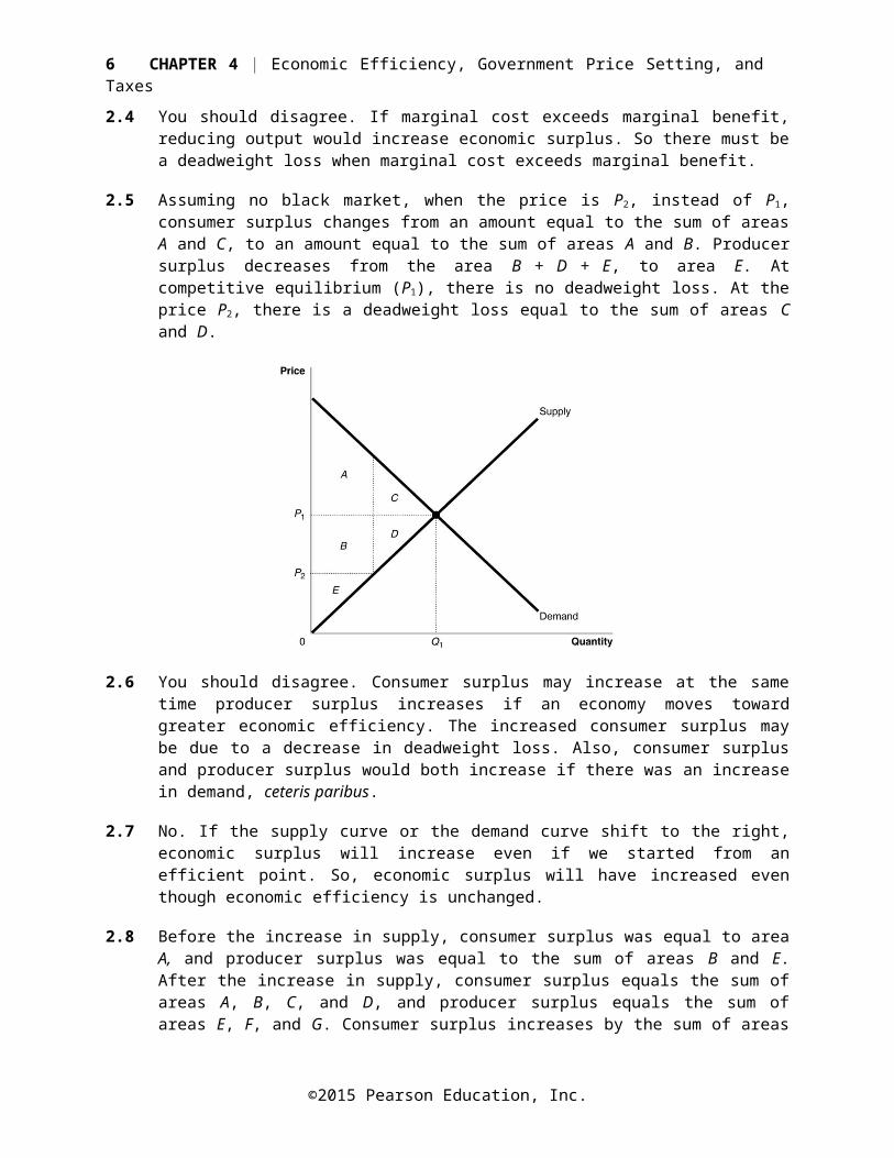
2.5 Assuming no black market, when the price is P2, instead of P1, consumer surplus changes from an amount equal to the sum of areas A and C, to an amount equal to the sum of areas A and B.


4


Producer surplus decreases from the area B + D + E, to area E. At competitive equilibrium (P1), there is no deadweight loss. At the price P2, there is a deadweight loss equal to the sum of areas C and D.

2.6 You should disagree. Consumer surplus may increase at the same time producer surplus increases if an economy moves toward greater economic efficiency. The increased consumer surplus may be due to a decrease in deadweight loss. Also, consumer surplus and producer surplus would both increase if there was an increase in demand, ceteris paribus.

2.7 No. If the supply curve or the demand curve shift to the right, economic surplus will increase even if we started from an efficient point. So, economic surplus will have increased even though economic efficiency is unchanged.

2.8 Before the increase in supply, consumer surplus was equal to area A, and producer surplus was equal to the sum of areas B and E. After the increase in supply, consumer surplus equals the sum of areas A, B, C, and D, and producer surplus equals the sum of areas E, F, and G. Consumer surplus increases by the sum of areas B, C, and D. Producer surplus increases by the sum of areas F and G but decreases by area B. So, producer surplus will increase if the sum of areas F and G is greater than area B. Economic surplus increases by the sum of areas C, D, F, and G.

2.9 You should disagree. It is not the difference between marginal benefit and marginal cost for a given level of output that is the key to economic surplus but whether marginal benefit exceeds marginal cost. Economic surplus increases as long as marginal benefit exceeds marginal cost for each additional unit of output. Economic surplus is greatest when the marginal benefit to consumers of the last unit produced is equal to its marginal cost of production.

2.10 At Q1, marginal benefit is greater than the marginal cost, so increasing output would increase economic surplus. At Q3, marginal cost is greater than marginal benefit, so reducing output would increase economic surplus.


5


4.3 Government Intervention in the Market: Price Floors and Price CeilingsLearning Objective: Explain the economic effect of government-imposed price floors and price ceilings.

Review Questions3.1 Some consumers gain from price controls because they can buy the product at a lower price, but

other consumers are hurt by price controls because shortages mean they are unable to buy the product.

3.2 Producers tend to favor price floors that are set above the equilibrium price, but only if producer surplus rises—as would be the case when the price rises a lot but the quantity sold doesn’t fall much. Producers don’t like price ceilings that are set below the equilibrium price because the quantity sold and the price received by producers both fall, reducing producer surplus.

3.3 A black market is one in which buyers and sellers violate government price regulations. A black market will arise if there are gains to some buyers and some sellers from violating a price floor or price ceiling.

3.4 Economic analysis will show the trade-offs involved from imposing price ceilings and price floors, but it won’t provide a final answer to the appropriateness of the policy because people differ about the goals of such policies. Some people may have the goal of maximizing economic surplus, for example, but others may care mostly about the well-being of certain consumers or producers and be less concerned about the well-being of other consumers or producers.

Problems and Applications3.5 a. 28 million crates

b. A surplus of 6 million crates (QD = 28, QS = 34, Surplus = QS – QD = 34 – 28 = 6 million crates)

c. The apple producers will benefit. Their revenue will increase from $8 × 30,000,000 = $240,000,000 to $10 × 28,000,000 = $280,000,000.

3.6 a. The equilibrium quantity is 100 million crates of kumquats per year and the equilibrium price is $20 per crate. Kumquat producers receive revenue of $2 billion.


6


b. Consumers will purchase 80 million crates of kumquats. Kumquat producers receive revenue of $2.4 billion, $30 × 80,000,000 = $2,400,000,000.

c. Kumquat producers will receive the revenue in part (b) plus $30 × 100 million crates, for a total of $5.4 billion. The government will spend $3 billion purchasing the 100 million crates of surplus kumquats. Or we can calculate directly the total amount kumquat producers will receive as $30 × 180 million crates = $5.4 billion.


7


3.7 a. PE is the competitive equilibrium price. PF is the price floor. Q1 is the quantity sold in competitive equilibrium. Q2 is the quantity sold with the price floor.

b. Economic surplus without a price floor = A + B + C + D + E. Economic surplus with price floor = A + B + D.

3.8 Whether the government should provide dependable income to dairy farmers is a normative judgment. Government officials are likely to use price floors and purchase the surplus of dairy products or provide financial incentives for dairy farmers to reduce supply. Whether government officials should use regulations to try to provide dependable income to every business is another normative judgment. The role of the economist is to indicate the effect of such policies on economic surplus (consumer plus producer surplus). It seems likely, though, that the government using price regulations to provide dependable incomes to every business would result in the market system no longer functioning. For a market system to function properly, most prices must be free to adjust to changes in demand and supply.

3.9 a. Price controls that make goods more affordable are price ceilings, which create shortages for the goods.

b. As shown in the graph below, the price ceiling causes a shortage for toothpaste and leads to a deadweight loss.


8


3.10 Black teenagers may be more affected by the minimum wage because they are relatively more likely to be working in industries and occupations where the unregulated wage would be so low as to make the minimum wage binding. This may be due to black teenagers possessing fewer skills, having less financial support at home, or being faced with discrimination. In addition, the minimum wage creates a surplus of workers, which allows employers who want to practice discrimination a greater opportunity to do so.

3.11 Renters who cannot rent apartments in Woburn will look for apartments in Peabody. As a result, the demand curve in Peabody will shift from D1 to D2, which will cause an increase in both equilibrium quantity and price in the market for apartments in Peabody.

3.12 If San Francisco repealed its rent control law, the prices for short-term rentals in San Francisco listed on Airbnb and other peer-to-peer sites would likely fall. Rent control causes a shortage of apartments and gives people an incentive to list their apartments on Airbnb or other sites at rents above the controlled rent. The reduced quantity of apartments resulting from rent controls raises the amount renters are willing to pay for a short-term rental. In effect, the reduced quantity of apartments moves prospective renters up their demand curves, raising the amount of rent they are willing to pay.

3.13 a. If someone is currently a renter, the law will probably make him or her better off, unless the landlord decides to remove the apartment from the market.

b. Probably worse off because the person will likely have difficulty finding a vacant apartment.

c. Worse off because the landlord will not be able to charge the competitive rent for apartments.

d. Probably better off because the landlord will be able to charge a higher rent than he or she would have been able to before the rent control law was passed. But the landlord may end up worse off if he or she gets caught and the penalty for breaking the law is large.

3.14 The statement is correct. If a good is not scarce (there is more freely available at zero price than we want), then there cannot be a shortage of the good. There is not a shortage of every scarce good, however. There is only a shortage of a scarce good when the price of the good is below the equilibrium price.


9


3.15 a. In the absence of rent control, the equilibrium price is $800, and the equilibrium quantity is 300,000. In this case, every renter who is willing to pay the market price of $800 will find an apartment, and every landlord willing to accept the market price of $800 will find a renter. The demand and supply curves are shown in the figure, along with the equilibrium price (PE) and quantity (QE).

b. At a price ceiling of $600, the quantity demanded is 350,000, but the quantity supplied is only 250,000, so there is a shortage of 100,000 apartments.

c. If all landlords abide by the law, the number of apartments rented will fall to 250,000. As shown in the figure, consumer surplus with the price ceiling enforced is A + C, producer surplus is E, and deadweight loss is B + D.

d. If landlords supply only 250,000 apartments and ignore the price ceiling, they can charge $1,000; $1,000 is the highest rent that consumers are willing to pay to rent 250,000 apartments.


10


3.16 The first sentence of the student’s argument is correct. The second sentence is incorrect. A price ceiling increases the quantity that consumers demand, but because it also reduces the quantity that sellers supply, it reduces the quantity of the product that consumers are actually able to buy. In the graph that follows, without a price ceiling, consumers buy Q1, but with a price ceiling, consumers buy only Q2.

3.17 a. The demand for hotels rooms, as shown in the figure below, increases during home football games. If prices for rooms are not allowed to rise above P1, which is the equilibrium price during weekends without home football games, during weekends with home football games there will be a shortage of hotel rooms equal to QD minus QS.

b. Out-of-town footballs fans will have trouble finding a hotel room. They will have to try to secure hotel rooms far in advance, secure hotel rooms in neighboring communities, drive home after the games, or not attend the games.

c. Over time, the supply of hotel rooms will most likely decline. With lower prices of hotel rooms reducing economic profits, some hotels will exit the industry. The exit of hotels makes the shortage of hotel rooms during home football game weekends more severe.


11


d. Ski resorts and vacation spots face peak seasons. Laws limiting the prices hotels can charge during peak seasons would decrease the quantity of hotel rooms available and, therefore, also decrease the number of tourists visiting these communities and spending money on local businesses.

3.18 a. After the decrease in supply, with no price ceiling, the equilibrium price would be $4.50, and the equilibrium quantity would be 40 million gallons. With a price ceiling of $3.50 and no black market, the price will be $3.50, the quantity demanded will be 45 million gallons, and the quantity supplied will be 30 million gallons, resulting in a shortage of 15 million gallons.

b. Consumer surplus = A + B + C, producer surplus = D, and deadweight loss = E + F.

c. Consumers are willing to pay, at most, $6.50 for the last gallon of gasoline suppliers are willing to supply at a price ceiling of $3.50. Consumer surplus = A, producer surplus = B + C + D, and deadweight loss = E + F.

d. Assuming there is no black market, some consumers are made better off by the price ceiling as they can purchase gas at a lower price than they otherwise could. However, some consumers will not be able to find gas at a price of $3.50 and will be worse off. Consumer surplus without the price ceiling is A + B + E, but with the price ceiling, it would be A + B + C. (C is larger than E even though it does not appear so in the graph because of scale adjustments. The area of E is ½ × 10,000,000 × $2.00 = $10,000,000, while the area of C is $1.00 × 30,000,000 = $30,000,000.)


12


3.19 a.

b. By legalizing the buying and selling of organs, the price would begin to rise, and the quantity supplied would also rise. As a result, the shortage of organs could be eliminated. However, by making the sale of kidneys legal, some members of society who are less educated or less well-informed might end up selling their kidneys even if it was not in their long-run best interest. There may be other solutions that would avoid the ethical problems of making kidney sales legal. Some economists, including Alvin Roth of Stanford University, have helped set up a kidney exchange that matches up compatible kidney donors and recipients.

4.4 The Economic Impact of TaxesLearning Objective: Analyze the economic impact of taxes.

Review Questions4.1 Tax incidence refers to the actual division of the burden of a tax between buyers and sellers in

a market.

4.2 A tax is efficient if it imposes a small excess burden (deadweight loss) relative to the tax revenue it raises.

4.3 The person who officially sends the tax revenue to the government need not be the one who actually bears the burden of the tax. For most taxes, the seller sends the money to the government, but buyers and sellers both pay part of the tax. The share paid by each depends on the slopes of the supply and demand curves and not on who is officially responsible for sending the tax to the government.

Problems and Applications4.4 In market equilibrium, the marginal benefit to consumers equals the marginal cost of production

of the last unit produced. A tax shifts the supply curve up vertically by the amount of the tax and


13


leads to a lower equilibrium quantity. At this lower quantity, the marginal benefit to consumers exceeds the marginal cost of production of the last unit produced. The deadweight loss is the reduction in units of output where the marginal benefit to consumers exceeds the marginal cost of production.

4.5

4.6 a. The tax is $1.25 per pack, which is represented by the vertical distance between S1 and S2.

b. Producers receive $4.25 per pack.

c. The government receives tax revenues of $1.25 × 18 billion = $22.5 billion a year.

d. Instead of the supply curve shifting up by the amount of the tax ($1.25), the demand curve would shift down by the amount of the tax ($1.25).

e. The new equilibrium price that buyers pay producers would be $4.25 per pack.

f. The total amount that cigarettes buyers pay per pack would be the price of $4.25 plus the tax of $1.25 for a total of $5.50, which is the same amount that buyers pay when the tax is collected from sellers.


14


4.7 This reasoning is incorrect. The demand curve for pizzas slopes downward, and the supply curve slopes upward, just as in other industries. So, as shown in the figure, the tax will be split between the buyers and sellers. The tax shifts the supply curve up from S1 to S2. The price paid by the buyers increases from PE to PB, while the after-tax price received by the suppliers decreases from PE to PS. PB – $1 = PS.

4.8 In most cases it is easier to collect the tax from sellers. There are fewer sellers than buyers, and it is easier to make sure that taxes are paid.

4.9 The $1 per hour of work payroll tax decreases the demand for labor by $1 at every quantity of labor. With a vertical supply curve for labor, the wage rate drops by the full $1 tax. Workers bear the full burden of the payroll tax. In the graph below, the equilibrium wage declines by $1 from W1 to W2.


15


4.10 a. The sum of areas D and G represent the excess burden (deadweight loss) of the tax.

b. The revenue collected by the government from the tax equals the amount of the tax (the vertical distance between S1 and S2) times the quantity sold after the tax is imposed (Q2), which equals the sum of areas B, C, E, and F.

c. The efficiency of the tax is be measured by the excess burden of the tax (the sum of areas D and G) relative to the tax revenue the tax raises (the sum of areas B, C, E, and F). This ratio of the excess burden and the tax revenue would have to be compared to the ratio of the excess burden to the tax revenue of other taxes to determine whether the tax on soft drinks is considered efficient.

Solutions to Chapter 4 Appendix4A.1 In a linear demand equation, the intercept on the price axis tells the price at which the quantity

demanded is zero. No consumer is willing to pay this price or above for the product. Similarly, in a linear supply equation, the intercept on the price axis tells the price at which the quantity supplied is zero. No firm is willing to produce the good at this price or less.

4A.2 The price that maximizes economic surplus is the equilibrium price. At this price there is no deadweight loss.

4A.3 Consumer surplus measures net benefit by subtracting the price paid from the total benefits received from the good or service.

4A.4 Deadweight loss is an interesting turn of phrase. It measures the loss of surplus, the gains to consumers and producers that could have been realized but were lost as a result of the price control (or other policy) that drags us away from efficiency like a heavy “weight” pulling the economy down.

4A.5 The equilibrium wage can be found by setting LD equal to LS and solving for W. 100 – 4W = 6W, so 100 = 10W, and W = $10. The equilibrium quantity of labor is LS = 6 × 10 = 60 thousand workers. The labor surplus equals LS − LD at the minimum wage. Plugging $12 into the supply equation: LS = 6 × 12 = 72. Plugging $12 into the demand equation LD = 100 – (4 × 12) = 52. Thus the surplus is 72 – 52 = 20 thousand workers.


16


4A.6 The minimum wage will have the larger impact on employment in the top figure. Because its demand curve is so flat, employers will reduce the quantity of labor demanded considerably more than in the right-hand figure.

4A.7 We can use the fact that at equilibrium QD = QS to determine the equilibrium price and quantity:

45 − 2P = 15 + P60 = 3PP = $20, Q = 45 − 2(20) = 5

So, the equilibrium price is $20 and the equilibrium quantity is 5. In the figure below, consumer surplus equals the area of A, or 0.5 × 5 × $2.50 = $6.25. Producer surplus equals the area of B, or 0.5 × 5 × $5 = $12.50.


17


4A.8 a. The deadweight loss from the price floor equals C + E. C = 0.5 × $1 × 10,000 = $5,000 and E = 0.5 × $1 × 10,000 = $5,000. So, deadweight loss = $10,000. Or, we can calculate the area of the deadweight loss triangle directly: ½ (20,000 – 10,000) × (3 − 1) = $10,000.

b. The price floor transfers area B from consumers to producers. The value of area B is $1 × 10,000 = $10,000.

c. Producer surplus after the price floor is imposed is equal to areas B + D + F = ($1 × 10,000) + ($1 × 10,000) + (1/2 × $1 × 10,000) = $25,000.

d. Consumer surplus after the price floor is imposed is equal to area A. The value of area A is ½ × $1.00 × 10,000 = $5,000.

4A.9 The totals are in millions of dollars.

Consumer surplus Producer surplus Deadweight loss

Competitive equilibrium

Rent control


Rent control


Rent control

$2,531 $3,120 $1,947 $985 $0 $374


18


With a rent ceiling of $2,000, the quantity supplied will be −1,000,000 + (1,300 × 2,000) = 1,600,000. The willingness to pay can be found from the demand equation: 1,600,000 = 4,750,000 – 1,000P, so 1,000P = 3,150,000 and P = $3,150.

Following Figure 4A.2 (page 133), consumer surplus under rent control equals its value in competitive equilibrium plus the value of area A minus the value of area B, producer surplus equals D, and deadweight loss equals B + C.

Area A = ($2,500 − $2,000) × 1,600,000 = $800,000,000

Area B = ½ × ($3,150 – 2,500) × (2,250,000 − 1,600,000) = $211,250,000, so

Consumer surplus = ($2,531,250,000 + $800,000,000) − $211,250,000 = $3,120,000,000

Deadweight loss equals Area B + C = $211,250,000 + 0.5 × ($2,500 - $2,000) × (2,250,000 – 1,600,000) = $373,750,000.

Producer surplus equals Area D = 0.5 × ($2,000 − $769) × 1,600,000 = $984,800,000.


19

Chapter 4nomadpress.com/.../omancoll/ccmicro/s/Ch04_solutions.docx · Web viewAnswers to Thinking...

Documents

Transcript of Chapter 4nomadpress.com/.../omancoll/ccmicro/s/Ch04_solutions.docx · Web viewAnswers to Thinking...