CHAPTER THREE

COUNT-BASED PVA: DENSITY-INDEPENDENT MODELS

Introduction..................................................................................................................................... 2

Population dynamics in a random environment.............................................................................. 2

The relationship between the probability of extinction and the parameters µ and 2σ ................. 5

Using count data to estimate the population growth parameters µ and 2σ - an illustration using the Yellowstone Grizzly Bear census ............................................................................................. 9

Estimating µ and 2σ as the mean and variance of ( )ii NN 1log + .......................................... 10

Estimating µ and 2σ by linear regression ............................................................................. 10

Regression procedure .......................................................................................................... 11

Using regression output to construct confidence intervals for µ and 2σ .......................... 12

Using regression diagnostics to test for temporal autocorrelation in the population growth rate....................................................................................................................................... 14

Using regression diagnostics to test for outliers.................................................................. 15

Using regression diagnostics to test for parameter changes................................................ 16

Using estimates of µ and 2σ to calculate the probability of extinction ..................................... 18

Using extinction time estimates for conservation analysis and planning ..................................... 20

Key assumptions of simple count-based PVAs ............................................................................ 21

Assumption 1 – The parameters µ and 2σ do not change over time..................................... 21

Density dependence............................................................................................................. 21

Demographic stochasticity .................................................................................................. 23

Temporal environmental trends .......................................................................................... 23

Assumption 2 – No environmental autocorrelation ................................................................. 24

Assumption 3 – No catastrophes or bonanzas.......................................................................... 24

Assumption 4 – No observation error ..................................................................................... 24

When to use this method............................................................................................................... 25

Tables............................................................................................................................................ 27

Boxes............................................................................................................................................. 31

Figure Legends.............................................................................................................................. 38

1

INTRODUCTION The type of population-level data that is most likely to be available to conservation planners and managers is count data, in which the number of individuals in either an entire population or a subset of the population is censused over multiple (not necessarily consecutive) years. Furthermore, to use such data for a PVA, it is not necessary to count the entire population; counts of breeding females, mated pairs, or plants actually in flower are all usable, as long as the segment of the population that is observed is a relatively constant fraction of the whole. Such data are relatively easy to collect, particularly in comparison with more detailed demographic information on individual organisms (see Chapters 6 through 9). In this chapter, we review a simple method for performing PVA using count data. The method’s simplicity makes it applicable to a wide variety of data sets. However, several important simplifying assumptions underlie the method, and at the end of the chapter, we discuss how violations of these assumptions would introduce error into our estimates of population viability. In the next two chapters, we review methods to handle those more complex situations. In a typical sequence of counts from a population, the observed number of individuals does not increase or decrease smoothly over time, but instead shows considerable variation around long-term trends (for an example, see Figure 3.6 later in the chapter). One factor that is likely to be an important contributor to these fluctuations in abundance is variation in the environment, which causes the rates of birth and death in the population to vary from year to year. As we mentioned in Chapter 2, the potential sources of environmentally-driven variation are numerous, including temporal variability in climatic factors such as rainfall, temperature, and duration of the growing season. Most populations will be affected by such variation, either directly or indirectly through its effects on interacting species (e.g. prey, predators, competitors, diseases, etc.). When we use a sequence of censuses to estimate measures of population viability, we must account for the pervasive effect of environmental variation that can be seen in most count data. To build a general understanding of how this is done, we first expand the overview of how environmental variation affects population dynamics that we gave in Chapter 2. We next review key theoretical results that underlie the simplest count-based methods in PVA. Then, with the necessary background in place, we delve into the details of using count data to assess population viability.

POPULATION DYNAMICS IN A RANDOM ENVIRONMENT Let us put more flesh on the bare-bones overview of how temporal variability influences population dynamics that we gave in Chapter 2. Specifically, let us return to the simple model for discrete-time geometric population growth in a randomly-varying environment Nt+1 = λt Nt (3.1) where Nt is the number of individuals in the population in year t and λt is the population growth rate, or the amount by which population size multiplies from year t to year t+1. Recall that Equation 3.1 assumes that population growth is density-independent (i.e., λt is not affected by population size, Nt). If there is no variation in the environment from year to year, then the population growth rate λ will be constant, and only three qualitative types of population growth are possible (Figure 3.1A): geometric increase (if λ>1), geometric decline to extinction (if λ<1), and stasis (if λ exactly equals 1). However, by causing survival and reproduction to vary from year to year, environmental variability will cause the population growth rate, λt, to vary as well,

2

and unlike the simple example in Chapter 2 in which we assumed λt only took on two values, in reality we expect λt to vary over a continuous range of values. Moreover, if the environmental fluctuations driving changes in population growth include an element of unpredictability (as factors such as rainfall and temperature are likely to do), then we will not be able to predict with certainty what the exact sequence of future population growth rates will be. As a consequence, even if we know the current population size and both the average value and the degree of variability in the population growth rate, the best we can do is to make probabilistic statements about the number of individuals the population will include at some time in the future. That is, we must view change in population size over time as a stochastic process. To illustrate stochastic population growth, Figure 3.1B shows 20 realizations of Equation 3.1 in which the value of the population growth rate λ was drawn at random each year1. All realizations start at a population size of 10 individuals. Thus each realization can be viewed as a possible trajectory the population might follow given its initial size and the distribution of λ. Figure 3.1B illustrates three fundamental features of stochastic population growth. First, the realizations diverge over time, so that the farther into the future you go, the more variable the predictions about likely population sizes become. Second, the realizations do not follow very well the predicted trajectory based upon the arithmetic mean population growth rate, λA (this is the trajectory shown by the upper smooth line in Figure 3.1B). In particular, even though in this case λA predicts that the population should slowly increase, a few realizations explode over the 20 years illustrated, whereas others decline. Thus extinction is possible even though the population size predicted by the arithmetic mean growth rate increases. Third, the endpoints of the 20 realizations shown are highly skewed, with a few trajectories winding up much higher than λA would suggest, but most ending well below this average prediction (in fact, three realizations ended lower than their starting population size). This skew is due in part to the multiplicative nature of population growth (see Equation 2.3). Because the size of the population after 20 years is proportional to the product of the population growth rates in each of those years, a long string of chance “good” years (i.e. those with high rates of population growth) can carry the population to a very high level of abundance, whereas strings of “bad” years tend to confine the population to the restricted zone between the average and zero abundance. We also saw in Chapter 2 that, because population growth is multiplicative, the geometric mean population growth rate λG is a better descriptor of the behavior of a typical realization. In fact, λG predicts the median population size at any point in the future; that is, for a large number of realizations, half will lie above and half below the population size predicted by λG (shown by the lower smooth line in Figure 3.1B; in this particular sample of 20 realizations, more happened to fall below the median than above, but λG still does a better job of “splitting the difference” than does λA). Skewness in the distribution of the likely future size of a population is a general feature of density-independent population growth in a stochastic environment. In fact, we can make an even more precise statement: the probability that the population will be of a certain size at a future time horizon will usually be well described by a particular skewed probability distribution, 1 Specifically, λ is lognormally distributed (that is, the log of λ follows the familiar normal distribution); the lognormal distribution is one of several distributions that can appropriately describe random λt values, because unlike the normal, it never takes on negative values, and to be biologically realistic, a discrete-time population growth rate should never be negative.

3

the lognormal2 (Lewontin and Cohen 1969). The particular lognormal distribution that would describe a large number of trajectories corresponding to the example in Figure 3.1B is shown in Figure 3.2 (compare this figure to Figures 2.4 and 2.5). The y-axis in Figure 3.2 is probability density; to obtain the actual probability that the population size lies between two particular values (the equivalent of the class boundaries in a histogram), we would calculate the integral of this probability density function between those two values of Nt. Thus population size is most likely to lie near the peak of the lognormal probability density function in Figure 3.2, but because the function is skewed to the right, the arithmetic mean population size will lie to the right of the peak. As Figure 3.2 illustrates, both the mean and the most likely population size increase over time, as does the probability density for larger population sizes. This makes sense given that most population trajectories tend to grow (Figure 3.1B). If population size itself follows a lognormal distribution, then the natural logarithm of population size will be normally distributed. This follows from the definition of a lognormal random variable; if Nt is lognormally distributed, then tt XN =log , where Xt is normally distributed3. As does the lognormal distribution of Nt values (Figure 3.2), the normal distribution of log Nt values will change over time (Figure 3.3). Specifically, its mean will either increase or decrease, depending on whether separate realizations of the stochastic population growth process tend to grow (as in Figure 3.1) or decline, but its variance will strictly increase (as prediction becomes less certain over longer time intervals). In this chapter, we will use log Nt, rather than the untransformed population size, because a normal distribution arises naturally from the physical process of diffusion, which we will use below to approximate the extinction process. Until now, we have talked about the growth of Nt. How do we characterize the growth of log Nt? Above and in Chapter 2, we argued that the best predictor of whether Nt will increase or decrease over the long term is λG, the geometric mean of the population growth rates each year. On the scale of log population size, the log of λG is the most natural way to express population growth. The geometric mean of λ is the value that would give the same average annual population growth rate as is observed over a long sequence of stochastically varying growth rates. That is, since 0012211 )( NN tttt λλλλλλ ⋅⋅⋅= −−+ (see equation 2.3), λG is defined as

or ( ) 01221 λλλλλλλ ⋅⋅⋅= −− tttt

G ( ) ttttG

/101221 λλλλλλλ ⋅⋅⋅= −− (3.2)

Converting this formula for λG to the log scale yields a new measure of “average” population growth4:

t

tttG

01221 logloglogloglogloglog λλλλλλλµ ++++++≈= −− (3.3)

As Equation 3.3 states, the correct measure of stochastic population growth on a log scale, µ, is equal to the log of λG or, equivalently, to the arithmetic mean of the log λt values. Thus if we can estimate the value of µ (which we will see how to do below), then we can immediately determine the geometric mean population growth rate, and thus whether the population will tend to grow or decline. In particular, Equation 3.3 predicts that if µ >0, then λG>1, and most population trajectories will grow, whereas if µ <0, then λG<1, and most trajectories will decline. 2 Thanks to the Central Limit Theorem, this conclusion is true asymptotically regardless of the probability distribution from which the λ’s are drawn. See Lewontin and Cohen 1969. 3 In this book, when we write “log” we always mean the natural logarithm (following mathematical convention). 4 Strictly speaking, the rightmost expression in Equation 3.3 approaches log λG only as t becomes large.

4

Because of this relationship between µ and λG, the parameter µ is of direct interest as a metric of population viability, telling us the direction in which the population will tend to move over time. But remember that even if µ is positive, there is still some chance that the population will fall to low levels, even to zero, as Figures 3.1B and 3.3A show. Thus in addition to knowing the population’s general tendency to grow or decline, we would also like to predict the full probability distribution for different population sizes, in particular so that we can calculate the probability that the population will fall below a specified quasi-extinction threshold at or before a specified future time horizon. To fully characterize the changing normal distribution of log population size (Figure 3.3), we will need two parameters. The parameter µ not only equals the log of λG ; it also represents the rate at which the mean of the normal distribution of log population size changes over time (that is, at time t, the mean of log Nt equals µ t; see Figure 3.3). But we must also define a second parameter, called (“sigma-squared”), that represents the rate at which the variance of the distribution increases over time (that is, at time t, the variance of log N

2σ

t equals t; Figure 3.3). Whereas 2σ µ is approximated by the (arithmetic) mean of the log population growth rates (i.e. the mean of the log λt values; see Equation 3.3), is approximated by the variance of the log λ

2σt’s, as we will see below. Our use of the symbol

to represent the variance of log λ follows Lande and Orzack 1988 and Dennis et al. 1991, the two most important sources for the material presented in this chapter. Throughout the book, we use

strictly to represent the variance in the log population growth rate that is caused by environmental stochasticity.

2σ

2σ

Together, µ and fully describe the normal probability distribution of future log population sizes. Specifically, a positive value of

2σµ indicates an environment in which most

realizations tend to grow, whereas a negative µ indicates that declining realizations predominate. The more the population growth rate λ varies from year to year as a result of environmental stochasticity, the greater will be the value of and the greater the range of possible population sizes in the future. These two measures of the dynamics of log population size are used extensively in the calculation of extinction times. Because their verbal definitions are somewhat tortuous (“the mean and variance of the log population growth rate”), we will usually refer to them by their symbols. Nonetheless, to really understand how simple count-based PVAs work, you will need to fix the meanings of

2σ

µ and in your mind. 2σ THE RELATIONSHIP BETWEEN THE PROBABILITY OF EXTINCTION AND THE PARAMETERS µ AND 2σ Because µ and describe the changing probability that the log population size will lie within a given range (Figure 3.3), it makes intuitive sense that if we know their values (as well as the current population size and the quasi-extinction threshold), we can calculate the probability of quasi-extinction at any future time. In this section, we review the theoretical underpinnings behind the calculation of extinction probabilities using

2σ

µ and . This section is more mathematically challenging than the rest of the chapter, and you may want to skip it. If you do, you will still be able to understand and use the following sections on how to do simple count-based PVAs, provided that you accept on faith the formulas relating

2σ

µ and to extinction risk. However, it is important to recognize the basic patterns in extinction times as well as the

2σ

5

assumptions underlying the theory, so we urge you to read the last three paragraphs of this section even if you skip the rest. For PVA purposes, we consider a population to be “extinct” (either literally so or at least in need of a radically different management approach) if it ever hits a quasi-extinction threshold. (In Chapter 2 we discussed several factors that determine the choice of a reasonable quasi-extinction threshold.) Thus to measure extinction risk, we want to calculate the probability that the population hits the threshold at any point during the interval between the present time and a specified future time horizon. We begin by calculating the probability that extinction first occurs in one small segment of that time interval, and then we sum the probabilities over all segments. This calculation is performed by viewing the changing normal distribution of log population size in Figure 3.3 as though it were a cloud of particles undergoing diffusion with drift. To envision this process, think of a large number of small beads released at a single point in an infinitely deep river, with height above the river bottom standing in for log population size. The path of each bead represents a single realization of “population” growth. As time evolves, the cloud of beads will move downriver, but its vertical position will change as well, moving upward or downward depending on whether the individual beads tend to float or sink, and spreading out due to turbulent flow of the water. The rate of floating or sinking is represented by µ , and the rate of turbulent diffusion by . The river bottom represents the quasi-extinction threshold; we will assume that any bead that hits the bottom will adhere to it (in mathematical terms, the quasi-extinction threshold is a so-called “absorbing lower boundary”). Even if the individual beads tend to float, some of them will be pushed to the bottom by turbulence, just as some population trajectories will hit low levels even as most trajectories tend to grow (Figure 3.3A), and the more turbulent is the flow of the water (i.e., the larger is ), the quicker some beads will be pushed to the bottom. Treating the change in log population size (or in the vertical position of a bead) as a process of diffusion with drift allows the rate at which realizations hit the lower boundary to be calculated (for full details on this diffusion approximation, see Cox and Miller 1965, pages 208-222, and Lande and Orzack 1988; for a clearly presented alternative derivation of Equation 3.4, see Whitmore and Seshadri 1987). Using a diffusion approximation, the probability density for hitting the quasi-extinction threshold (that is, going “extinct”) in a small segment of time beginning at t is given by the so-called “inverse Gaussian” distribution

2σ

2σ

5:

( )⎟⎟⎠

⎞⎜⎜⎝

⎛ +−=

ttd

tddtg 2

2

32

2

2exp

2),,(

σµ

πσσµ (3.4)

where is the difference between the log of the current population size Nxc NNd loglog −= c and the log of the extinction threshold, Nx. (The notation ),,( 2 dtg σµ means that the value of g at

time t depends on the values of µ , , and d.)2σ Notice that the extinction probability depends only on the difference (on the log scale) between the current and threshold population sizes, not on their actual values. 5 Strictly speaking, Equation 3.4 is a “proper” probability distribution (i.e. a function that integrates to 1) only if µ<0. This merely reflects the fact that when µ>0, not all realizations hit the threshold, so the ultimate probability of extinction is less than 1 (see Equation 3.7). Equation 3.4 can be converted into a proper probability distribution for the time to hit the threshold given that the threshold is reached eventually by replacing the numerator of the exponential term by –(d–|µ|t)2. However, the “improper” distribution is actually more useful to us, as it reflects the full, unconditional probabilities of extinction. See Lande and Orzack 1988.

6

Figure 3.4 illustrates how the shape of the inverse Gaussian distribution (Equation 3.4) is affected by the values of µ and . The most likely time to hit the threshold is the peak of the distribution. The position of the peak is shifted toward shorter times as the value of increases (compare curves with the same value of

2σ2σ

µ but different values of ). This is because greater variation drives populations down to the threshold more rapidly, as we would expect from the analogy with diffusing beads. Figure 3.4A shows that more negative values of

2σ

µ lead to shorter quasi-extinction times (compare the two curves with =0.04). This also makes sense; if the mean of the normal distribution of log population size declines more rapidly, quasi-extinction should occur earlier. If

2σ

µ is positive, the probability of quasi-extinction occurring in each time segment is smaller than if µ is negative (compare Figure 3.4 A&B, and note the different scales of the y-axes), and the more positive µ is, the smaller is the total area under the curve (which represents the ultimate probability of quasi-extinction, as we will see below). However, notice that as µ becomes more positive, the peak of the distribution (i.e. the most likely quasi-extinction time) actually decreases (compare curves for µ =0.01 and µ =0.03 with the same value of in Figure 3.4B). The reason for this somewhat counter-intuitive result (as explained by Lande and Orzack 1988 and Dennis et al. 1991) is that when

2σµ is

strongly positive, most realizations tend to increase rapidly to high numbers, from which they are unlikely to ever hit the quasi-extinction threshold. It is only early in the growth process, when population size is still low, that a chance string of bad years can push the population down to the threshold. So, extinction is unlikely to happen, but if it does, it will occur rapidly. The inverse Gaussian distribution gives the probability that quasi-extinction occurs in a very small time segment. To calculate the probability that the threshold is reached at any time between the present (t=0) and a future time of interest (t=T), we integrate Equation 3.4 from t=0 to t=T (that is, we sum up the probabilities for each small interval of time). The result is the cumulative distribution function (or CDF) for the time to quasi-extinction,

( ) ⎟⎟⎠

⎞⎜⎜⎝

⎛ +−Φ−+⎟⎟

⎠

⎞⎜⎜⎝

⎛ −−Φ=

TTdd

TTddTG

2

2

2

2 2exp),,|(σ

µσµσ

µσµ (3.5)

where Φ(z) (“phi”) is the standard normal cumulative distribution function

( ) ( )dyyzz

∫ ∞−−=Φ 2exp21)( 2π (3.6)

Φ(z) is simply the area from to z under a normal curve with a mean of zero and a variance of 1. Values of Φ(z) are tabulated in most basic probability reference books (e.g. Abramowitz and Stegun 1964), and can be calculated using built-in functions in mathematical software packages such as MATLAB and even spreadsheet programs such as Excel.

∞−

Figure 3.5 illustrates how the probability of hitting the threshold according to Equation 3.5 increases as the time horizon T is moved farther into the future. If µ is substantially negative, the probability of extinction increases rapidly with time, quickly reaching a value near 1. If the time horizon is not far into the future, increasing the value of increases the probability that extinction will have occurred before the horizon is reached (once again, greater year-to-year variability leads to higher extinction risk). For positive

2σ

µ , the probability of extinction increases slowly with time, and never reaches a value of 1. The probability of ultimate extinction (that is, at a time horizon of infinity) can be calculated by taking the integral of the inverse Gaussian distribution from t=0 to t= ∞ :

7

( )⎩⎨⎧

>−≤

=∞02exp01

),,|( 22

µσµµ

σµifdif

dG (3.7)

Thus if µ is zero or negative, ultimate extinction is certain, and increasing has no effect on the probability that the threshold is eventually reached. In contrast, if

2σµ is positive, ultimate

extinction is not a certainty, and increasing increases the probability of ultimate extinction. 2σ While the rest of this chapter is devoted to the calculation of extinction risk estimates for quantitative data, even in the absence of any data, knowledge of how the CDF is affected by its underlying parameters can help us to make useful qualitative assessments of relative viability for a species of critical concern, especially if we can use natural history information to make inferences about the local environment or about the life history of the species in question. For example, we will frequently be able to make an educated guess that the environment one population experiences is likely to be more variable than another’s in ways that will affect population growth. Such differences in influence the extinction time CDF even when its other determinants (µ and the starting and threshold population sizes) are fixed (Figure 3.5). Similarly, some species will have life history features (e.g. long-lived adults) that buffer their populations against year-to-year environmental variation, while others do not. With a low , values of µ that are only slightly positive are sufficient to minimize extinction risks, while with high variance, much greater mean growth is needed. Thus we can state that, all else being equal, the greater the environmentally-driven fluctuations in population growth rate the greater will be the risk of extinction, especially for short-term time horizons, a statement that, though qualitative, nonetheless provides some useful guidance.

2σ

2σ

Before going on, it is also important to recognize that three key assumptions underlie the use of a diffusion approximation to derive the key Equations 3.4, 3.5, and 3.7. First, we assume that the environmental perturbations affecting the population growth rate are small to moderate, just as gas molecules typically diffuse through a series of small jumps6. In other words, we assume that large catastrophes or bonanzas (Chapter 2) do not occur frequently enough to be important. Second, we assume that the changes in population size are independent between one time interval and the next; that is, we assume that strings of good or bad years occur no more frequently than would be expected by chance. Third, we assume that the values of µ and do not change over time, either in response to changes in population density or because of temporal trends in environmental conditions. We show how to test for violations of these assumptions in

2σ

6 Technically, diffusion models also assume that the state variable (in this case population size) is continuous, whereas in reality, a population can only contain an integer number of individuals. The assumption of small environmental perturbations is therefore tantamount to assuming that the change in numbers over a short time interval relative to the total number of individuals in the population is small, as assumption that is likely to break down at small population sizes (Ludwig 1996a). Using a moderate quasi-extinction threshold, as we advocated in Chapter 2, ameliorates to some extent the effects of this assumption.

8

the following section, and how to deal with some of these violations (should they occur) in Chapter 4.

USING COUNT DATA TO ESTIMATE THE POPULATION GROWTH PARAMETERS µ AND - AN

ILLUSTRATION USING THE YELLOWSTONE GRIZZLY BEAR CENSUS

2σ

We argued in Chapter 2 that the extinction time cumulative distribution function or CDF, given by Equation 3.5 and illustrated in Figure 3.5, is perhaps the single most useful metric of a population’s risk of extinction. To calculate it, we need only four quantities: the current population size Nc, the extinction threshold Nx, and the values of µ and . We turn now to methods for estimating

2σµ and from a series of census counts. 2σ

Let us assume that we have conducted a total of q+1 annual censuses of a population at times , , , …, , having obtained the census counts , , , …, . The censuses need not have been conducted in consecutive years, but in a seasonal environment, the censuses should have been performed at the same time of year. While

0t 1t 2t qt 0N 1N 2N qN

µ and can be used to describe future population size distributions (as shown in Figure 3.3), they are more directly measures of the mean and variance of the change in log population sizes. Thus it is not the raw census counts themselves that we want to use to estimate

2σ

µ and , but the amount by which the natural logarithms of the counts change over each of the inter-census intervals. For example, over the time interval of length

2σ

( )ii tt −+1 years between censuses i and i+1, the logs of the counts change by an amount

( ) iiiii NNNN λloglogloglog 11 ==− ++ (3.8) In Equation 3.8, iii NN 1+=λ is the population growth rate between census i and census i+1, emphasizing the fact that it is the logs of the population growth rates that we will use to estimate µ and . The counts from q+1 censuses allow us to calculate log population growth rates for q time intervals, although as noted above, these intervals need not be of the same length.

2σ

An example of count-based data that we will analyze extensively in this chapter comes from the ongoing census of adult female grizzly bears (Ursus arctos) in the Greater Yellowstone Ecosystem (for an earlier analysis of the same population, see Dennis et al. 1991). This population is currently designated as threatened by the United States Fish and Wildlife Service, and is completely isolated from other grizzly bear populations. Each year, bear biologists count the number of unique female bears with cubs (offspring in their first year of life) in the entire Yellowstone population. Because the litters of one to three cubs remain closely associated with their mothers, females with cubs are the most conspicuous, and therefore most reliably censused, element of the population. Censuses were originally performed by observing bears at park garbage dumps, but they have been conducted by aerial survey since the closure of the dumps in 1970-1971. The counts of females with cubs are used to estimate the total number of adult females in the population. Specifically, the number of adult females in year t is estimated as the sum of the observed number of females with cubs in years t , t+1, and t+2 (Eberhardt et al. 1986). The logic underlying this estimate is that the interval between litters produced by the same mother is at least three years, so that females with cubs observed in years t+1 and t+2 could not have been the same individuals that were observed with cubs in year t. Yet, if they are observed in later years, they must have been alive in year t (although they may not have been

9

adults in year t, which introduces some error). The estimated numbers of adult females from 39 annual censuses of the Yellowstone population, beginning in 1959, are shown in Figure 3.6 and listed in Table 3.1 (these data can also be obtained at the Interagency Grizzly Bear Study Team's website: www.nrmsc.usgs.gov/research/igbstpub.htm).

We now review two methods to estimate µ and , illustrating both methods with the grizzly bear data in Table 3.1.

2σ

Estimating µ and as the mean and variance of 2σ ( )ii NN 1log +

If the censuses were conducted at regular yearly intervals, as was the Yellowstone grizzly bear census, the simplest method of estimating µ and is to calculate the arithmetic mean and the sample variance of the

2σ( ii NN 1log + ) values, given respectively by

(∑−

=+=

1

01log1ˆ

q

iii NN

qµ ) and ( )(

21

01

2 ˆlog1

1ˆ ∑−

=+ −

−=

q

iii NN

qµσ ) (3.9)

(where the hats over µ and indicate that they are estimates). Notice that in calculating , we divide by q−1 instead of q, thus using the typical formula to obtain an unbiased estimate of variance from a sample of data (Dennis et al. 1991

2σ 2σ

7). The values of µ and are easily obtained by applying the functions AVERAGE and VAR (respectively) in Microsoft Excel to the

2σ

( ii NN 1log + ) values, or by using similar routines in any statistical package. The estimates µ and for the Yellowstone grizzly bear calculated using Equations 3.9

are given in Table 3.1. The value of

2σµ is positive, reflecting a general upward trend in the

number of adult female bears over the sampling period (Figure 3.6). The value of is about 60% of the value of

2σµ ; recall that is a measure of the year-to-year variability in the census

counts.

2σ

Estimating µ and by linear regression 2σ

If the censuses were not taken at equal time intervals, we should not use Equations 3.9 to

estimate µ and , because they do not account for the fact that both the mean and variance in population change should be larger for pairs of censuses that are separated by longer intervals of time

2σ

8. In such cases, we can estimate the parameters using a linear regression method proposed by Dennis et al. (1991). In fact, the linear regression method, although somewhat more complicated to execute, has advantages over Equations 3.9 even when the censuses occurred every year. In particular, the output produced by most widely-available regression packages allows us to easily place confidence limits on the parameters and to test assumptions of the underlying PVA model, as we now demonstrate.

7 We use the symbol to represent the unbiased estimate of . Dennis et al. (1991) use 2σ 2σ 2~σ . 8 An alternate formula that does account for the length of the time interval is presented in Dennis et al. 1991 (see their Equations 24 & 25), but as it does not have the advantages of their regression approach, we do not present it here.

10

Regression procedure The basic idea of this method is to regress the log population growth rate over a time

interval against the amount of time elapsed. However, the most straightforward way to do this does not conform to one of the assumptions of standard linear regression, namely that the variance in the dependent variable (log population growth, in this case) is constant over different values of the independent variable (time elapsed). As we noted above, the variance of log population size increases with time (see Figure 3.3), which means that the variance in population change over a time interval is also dependent on the time elapsed. In particular, if two censuses are separated by years, then ii tt −+1 ( )ii NN 1log + has a variance of . To make our regression conform to the assumption of equal variances, we need to transform the rate of population change (and also the time elapsed) to get rid of this time dependence. This is accomplished by dividing both the log population growth rate and the time elapsed by

)( 12

ii tt −+σ

ii tt −+1 ,

which makes the variance in the transformed population change variable equal to for any time interval.

2σ

Thus, to perform the linear regression, we first calculate a transformation of the length of each time interval to use as the independent variable:

iii ttx −= +1 . (3.10a) We then calculate a transformed variable of population change, the dependent variable, as:

( ) ( ) iiiiiiii xNNttNNy 111 loglog +++ =−= . (3.10b) For example, if we have entered the values of ti and Ni from Table 3.1 in the first 39 rows of Columns A and B in an Excel worksheet, we can perform the transformations in Equations 3.10a,b by entering the formulas =SQRT(A2-A1) in cell C1 and =LN(B2/B1)/C1 in cell D1 and then “filling down” the subsequent 38 rows of Columns C and D. Notice that when all adjacent censuses are one year apart, as in the grizzly bear data set, all the x values will equal 1, and yi will equal ( )ii NN 1log + .

The final step is to perform a linear regression of the yi’s against the xi’s forcing the regression intercept to be zero (in some statistics packages, such as Excel’s regression routine, this is accomplished by choosing “no constant” in the regression options). By fixing the regression intercept at zero, we are enforcing the rule that there can be no change in population size if no time has elapsed. The slope of the regression is an estimate of µ and the regression’s error mean square estimates (Figure 3.7). For example, the following SAS command ato the transformed grizzly bear data generates the output in Box 3.1:

2σ pplied

proc reg;

model y=x / noint dw influence; (3.11) run;

The command noint induces a regression with no intercept, and the commands dw and influence instruct SAS to print regression diagnostics of which we will make use below. In Box 3.1, the “Parameter Estimate for the Variable X” (0.021337) is the regression slope, which is our estimate of µ , and the second entry (0.01305) in the column “Mean square” in the Analysis of Variance table is the error mean square, which is our estimate of . The output in Box 3.1 is equivalent to that produced by virtually all good statistics packages, although terminology may differ (for example, the error mean square is sometimes labeled “residual mean square”). Notice that the regression yields the same estimates for

2σ

µ and that we obtained in 2σ

11

Table 3.1. However, the regression output also provides additional useful information, as we now review.

Using regression output to construct confidence intervals for µ and 2σ Ideally, we want more than just the single best estimates of µ and . Because these will only be estimates based on the limited number of transitions in the data set, we would also like to know how much confidence we can place in them. Confidence intervals provide an upper and lower value between which the true value of each parameter is likely to lie. Confidence limits help us to place the best estimates of each parameter in context. For example, if

2σ

µ , the best estimate of µ , is positive, we would predict that most population trajectories will grow (as in Figure 3.3A). However, if the lower limit of the confidence interval for µ is negative, we cannot, based on the available data, rule out the possibility that the population will actually tend to decline over the long term.

In a proper linear regression, the estimate of the slope (i.e. µ , the estimate of µ ) is normally distributed around its true value. Using this fact, many statistics packages will provide 95% confidence limits or standard errors for the regression slope. If yours does not, or if you want to calculate different confidence limits (say, 90 or 99% limits) it is easy do so to using the following formula: ( ))ˆSE(ˆ),ˆSE(ˆ 1,1, µµµµ αα −− +− qq tt (3.12) (Dennis et al. 1991). Here, is the critical value of the two-tailed Student’s t distribution with a significance level of α and q−1 degrees of freedom. For example, if we want to place a 95% confidence interval around

1, −qtα

µ for the Yellowstone grizzly bear, we would set α equal to 0.05 and q equal to 38 (the number of transitions on which the regression was performed; Table 3.1), and then obtain the value of . We can look up this value in most standard statistics texts or compute it with the aid of mathematical software such as MATLAB

37,05.0t9; even many

spreadsheet programs can calculate it. For example, entering the formula =TINV(0.05, 37) into a cell in a Microsoft Excel worksheet yields the value =2.0262. In Equation 3.12, 37,05.0t )ˆSE(µ is the standard error of µ , the estimated regression slope. SAS supplies it in the regression output (Box 3.1) in the column labeled “Standard Error”; it is 0.0185. The standard error can also be calculated directly from the expression qt

2σ , where is the regression error mean square and t

2σ

q is the duration of the census in years (Dennis et al. 1991); for the Yellowstone grizzly bear data in Table 3.1, the census spans tq =38 years, from 1959 to 1997. Substituting the values of µ , , and 37,05.0t )ˆSE(µ that we have just calculated into Expression 3.12 gives us a 95% confidence interval of (−0.01621, 0.05889) for the parameter µ . The way to view this confidence interval is to imagine repeatedly sampling at random 38 log growth rates from this population; the confidence intervals computed using Equation 3.12 would include the true value 9 Specifically, the MATLAB function tinv will compute the inverse t statistic, but users must purchase the Statistics Toolbox to use tinv.

12

of µ 95% of the time. The fact that the confidence interval we have calculated ranges from negative to positive values indicates that, despite strong growth of the population in recent years (Figure 3.6) and the relatively long-term nature of the census, we still cannot rule out the possibility that the population will decline. Notice that the regression output in Box 3.1 also provides a test of the null hypothesis that the slope of the regression is zero. The relatively large probability associated with this test (0.2570) also tells us that we cannot say definitively that the population is growing, even though µ is positive. The results in the preceding paragraph highlight an important conservation lesson: we should be very skeptical about single estimates of viability metrics that are presented without an associated measure of uncertainty, such as a confidence interval. The case of the Yellowstone grizzly bear is particularly apropos. Recent years have witnessed intense pressure to remove the Yellowstone grizzly bear population from the Endangered Species list; much of that pressure is motivated by a desire to show that the Endangered Species Act functions effectively to bring about recovery of threatened and endangered species and populations. However, our analysis shows that it would be dangerous to conclude from the data in Table 3.1 that, because the best estimate of µ is slightly positive, the Yellowstone grizzly bear population is growing and can be safely delisted. The lower confidence limit on µ says that such a conclusion would be premature. To know how much confidence we can place in extinction probabilities based on the estimated values of µ and , we also need to calculate a confidence interval for . Such an interval can be constructed using the chi-square distribution (Dennis et al. 1991). For example, if we want to place a 95% confidence interval around for the Yellowstone grizzly bear, for which we have data on q=38 transitions, we first obtain the 2.5

2σ 2σ

2σth and 97.5th percentiles of the chi-

square distribution with q−1=37 degrees of freedom: call them and . Once again, these can be looked up in a statistics reference or calculated with the aid of MATLAB

237,025.0χ 2

37,975.0χ10 or

a spreadsheet program; the Excel formulae =CHIINV(0.025, 37) and =CHIINV(0.975, 37) yield the values = 55.6680 and = 22.1056. We substitute these values into the

following general expression for a 95% confidence interval for based on q-1 degrees of freedom:

237,025.0χ 2

37,975.0χ2σ

( )21,975.0

221,025.0

2 ˆ)1(,ˆ)1( −− −− qq qq χσχσ (3.13) (Dennis et al. 1991). Note that we can use this same approach to calculate confidence intervals with other degrees of coverage. For example, to calculate a 90% rather than a 95% confidence interval, we would substitute the values of and into the first and second terms in Equation 3.13, respectively.

21,05.0 −qχ 2

1,95.0 −qχ

For the Yellowstone grizzly bear, Equation 3.13 gives us the confidence interval (0.00867, 0.02184) for . Thus a true value of nearly 70% higher than the best estimate of

=0.01305 is consistent with the available data (as is a much smaller value). We will return to Equations 3.12 and 3.13 when we discuss how to incorporate parameter uncertainty into estimates of extinction probabilities.

2σ 2σ2σ

10 Specifically, you can use the function chi2inv if you have purchased MATLAB’s Statistics Toolbox.

13

Using regression diagnostics to test for temporal autocorrelation in the population growth rate Another advantage of estimating the parameters µ and by regression is that we can test the assumption of the diffusion approximation that the environmental conditions (and thus the log population growth rates) are uncorrelated from one inter-census interval to the next (that is, whether a particular interval was good or bad for birth or death is independent of whether preceding or succeeding intervals were good or bad). One test makes use of the Durbin-Watson d statistic (invoked by the DW option in SAS), which measures the strength of autocorrelation in the regression residuals (and we are interpreting the residuals as being the result of environmental perturbations). A residual is simply an observed value of y (i.e., the value of

2σ

( ) iiii ttNN −++ 11log for census i) minus the value predicted by the regression equation (which

equals ii tt −+1µ ). The two-tailed Durbin-Watson test evaluates the null hypothesis that all of the serial autocorrelations of the residuals are zero (Draper and Smith 1981). To perform the test, we compare both d and 4−d to upper and lower critical values dL and dU. Specifically, if d<dL or 4−d<dL, we conclude that the residuals show significant autocorrelation; if d>dU and 4−d >dU, we conclude there is no significant autocorrelation; and otherwise, the test is inconclusive. Values of dL and dU for a significance level of α=0.05 and different numbers of data points in the regression, q, are given in Table 3.2; for other values of q, dL and dU can be calculated by linear interpolation, or by referring to Table 3.3. in Draper and Smith 1981. For the Yellowstone grizzly bear, q=38, so that dL=1.33 and dU=1.44. The calculated value of d is 2.57 (Box 3.1). Because d>dU but 4−d nearly equals dU, this value of d leads to a test result that is right on the border between inconclusive and a finding of no significant autocorrelation. We conclude that there may be some autocorrelation in the residuals, but that it is probably weak. Another sign that the autocorrelation in the residuals is at best weak is the fact that the first-order autocorrelation of the residuals11 (r=−0.288 with 37 degrees of freedom; see Box 3.1) has a small but non-significant p value (p=0.084; this p value is calculated by most statistical packages and can be looked up in tables of two-tailed significance levels of the Pearson correlation coefficient, given in most basic statistics references). Given the possibility that successive log population growth rates may be slightly correlated (in this case negatively), a thorough analysis 11 This autocorrelation can be computed easily as follows. Place the residuals for years 1 to q−1 in one column of a spreadsheet, and the residuals for years 2 to q in the adjacent column. Then compute the Pearson correlation coefficient of the two columns of numbers. SAS performs this calculation for you when you specify the DW option in PROC REG (see Box 3.1).

14

of the data should include an examination of the possible effect of the observed level of autocorrelation on the estimated viability of the grizzly bear population, using methods we describe in Chapter 4.

Using regression diagnostics to test for outliers We can also use the regression output to evaluate whether any particular transitions are outliers or are having a disproportionate influence on the parameter estimates. There are a variety of measures of the importance of a data point on the results of a regression. These include Cook’s distance measure, leverage, and studentized residuals; different statistics packages provide different combinations of these measures. For example, the “influence” option in PROC REG of SAS produces an output table with two useful measures of the effect of each data point on the regression results (Box 3.1). The column labeled “Rstudent” gives the studentized residual for each (x,y) pair in the regression. Data points with studentized residuals greater than 2 are suspected outliers (SAS 1990). “Dffits” is a statistic that measures the influence each data point has on the regression parameter estimates; for a linear regression with no intercept, a value of Dffits greater than q12 (where q is the number of data points, or transitions) suggests high influence (SAS 1990). For the grizzly bear data set, the critical value of Dffits is 324.03812 = . By both the studentized residual and Dffits criteria, the 25th transition in the data set, corresponding to the 1983-1984 censuses, is flagged as an unusually large transition with a high influence on the estimate of µ . This transition represents a large proportional increase, in which the counts grew by more than 50% in a single year (Figure 3.6). Dennis et al. (1991) identified this same transition as an outlier in their analysis of the 1959-1987 census data. If an outlier or influential observation is identified in your data set, you must decide whether to keep that data point or remove it from the regression. To make this decision, we recommend first examining why that point may be unusual. If the cause is “non-biological”, it might be sensible to delete the data point. For example, if unusual transitions are associated with years in which methodological problems with the census were known to have occurred, or if they correspond to a change from one method of censusing the population to another, they may represent errors in the counting process rather than periods of unusually high or low population growth. As we want our parameter estimates to include real environmental variation but to exclude observation error as much as possible (see Chapter 5), deleting such points would be justified. In the case of the Yellowstone grizzly bear, we are not aware of any such problems that occurred in the 1983 or 1984 censuses; hence we see no reason to delete the 25th transition as being unduly influenced by observation error. On the other hand, there may be real biological reasons why a particular transition is an outlier. These reasons can be classified as one-time human impacts and extreme environmental conditions; how we should treat these two types of outliers differs. If an outlier can be pegged to a one-time human impact that we do not expect to recur, that outlier should be omitted for the purposes of predicting the future state of the population. A hypothetical example of such an impact on the Yellowstone grizzly bear would be effects of closing the park garbage dumps (at which the bears had become accustomed to scavenge for food). Because this event is unlikely to occur again, any unusual transitions associated with it should not be allowed to influence our

15

predictions for the future. The unusually high 1983-1984 transition, however, is not likely to be related to the closure of the dumps, which occurred in 1970-1971. Finally, outliers could represent the consequences of extreme environmental conditions, either catastrophes or bonanzas (Chapter 2). Recall that the diffusion approximation used to derive an expression for the cumulative probability of extinction (Equation 3.4) assumed that such large fluctuations in the population growth rate do not occur. Strictly speaking, then, we should not use Equation 3.5 to calculate an extinction probability if our estimates of µ and have been influenced by catastrophes or bonanzas. Instead, we must resort to computer simulation to calculate extinction probabilities, as we describe in Chapter 4.

2σ

In the case of the Yellowstone grizzly bear, the only suspected outlier is an unusually large increase in population size. Large increases inflate the estimated values of both µ and

. As a higher value of 2σ µ reduces the probability of extinction but a higher value of increases it (Figure 3.5), it is not clear how these two effects of the outlier on the extinction probability play out. Because of this, and because no environmental factors that could have caused the 1983-1984 transition to be a bonanza have been identified, we have chosen to retain this transition when estimating

2σ

µ and . However, readers are encouraged to explore how the probability of extinction changes if we use parameter estimates (

2σµ =0.01467 and =0.01167)

obtained after deleting the 25

2σth transition.

As the foregoing discussion indicates, there is no general rule regarding when to omit outliers, and the decision to do so must be decided on a case-by-case basis. Our point here is simply that the regression approach makes this decision possible by identifying outliers in the first place. When outliers are omitted, it is important that you state this fact explicitly in any reports you prepare on your PVA results, and that you carefully document why those points were omitted.

Using regression diagnostics to test for parameter changes A final advantage to the linear regression approach is that it provides a way to ask if µ or

differ significantly in distinct segments of the time series. For example, for the Yellowstone grizzly bear, we might ask whether the parameter estimates differ before vs. after the closure of the garbage dumps in 1970-1971, or before vs. after the 1988 Yellowstone fires.

2σ

To test for changes in µ and before vs. after a pivotal census (e.g. 1988, the year of the fires), we recommend that you perform linear regressions in the following order. The first step is to test for differences in before and after the pivotal census. To do this, divide the transitions into those leading up to and including the pivotal census vs. those from the pivotal census onward. Transform each data set using Equations 3.10a,b. Next, perform separate linear regressions with zero intercept on these two transformed data sets (e.g. using two repetitions of SAS Command 3.9 above) to obtain two estimates of , call them and (the subscripts here stand for “before” and “after”). For example, if we divide the Yellowstone grizzly bear censuses into “before-fire” (1959-1988) and “after-fire” (1988-1997) periods, we obtain the estimates = 0.01229 and =0.01561 from the error mean squares of the separate regressions. There are 29 and 9 transitions in these two data sets, respectively. We can perform a two-tailed test for a significant difference between two variances (in this case and ) by

2σ

2σ

2σ 2ˆ bσ 2ˆ aσ

2ˆ bσ 2ˆ aσ

2ˆ bσ 2ˆ aσ

16

calculating their ratio with the larger variance in the numerator, and computing its probability from an F distribution with the appropriate numerator and denominator degrees of freedom (Snedecor and Cochran 1980). For the grizzly bear data, the ratio / =1.270 has 9−1=8 numerator and 29−1=28 denominator degrees of freedom. The probability of observing a ratio this large or larger if the two data sets have the same true value of is 0.298 (obtained from an F table in any statistics reference or by using the Excel formula =FDIST(1.270,8,28) ). As this probability is larger than 0.025

2ˆ aσ 2ˆ bσ

2σ

12, we conclude that there is no significant difference in the degree of variability in the grizzly bear population growth rate before vs. after the 1988 Yellowstone fires.

Had the values differed, we would use the two separate regressions to make different estimates of both

2σµ and , and conduct any analysis of future trends using only the more

recent set of estimates (unless for some reason we thought that the earlier population dynamics might be a better indicator of what will happen in the future, for example if a threat to the population that was present only during the later time interval has now been removed). In this case, however, we have determined that does not differ significantly before vs. after the fires, but we still need to test for differences in

2σ

2σµ while allowing only a single estimate of that

applies to the entire census. We can do this by creating two x variables (call them x

2σ1 and x2) and

performing a multiple linear regression of y on x1 and x2, once again forcing the regression to have an intercept of zero (Dennis et al. 1991). The new variable x1 will have the values of xi calculated from Equation 3.10a for all years before the fires and zero for all years after the fires. In contrast, variable x2 will be zero for years before the fires and have values calculated from Equation 3.10a for all years after the fires. The y values should be computed from Equation 3.10b as before. The following SAS command performs this multiple regression of y on x1 and x2, yielding the output in Box 3.2:

proc reg;

model y=x1 x2 / noint; (3.14) run;

The parameter estimates associated with variables x1 and x2 give us bµ =0.01069 and

aµ =0.05564 for the periods before and after the fires, respectively. The single estimate of for the entire census, once again obtained from the error mean square, is =0.01303 (the subscript m here indicates that this estimate was obtained from a multiple regression; it is not necessarily the same as the estimate obtained from a single regression, as in Box 3.1). As the

2σ2ˆ mσ

estimates of a regression slope are normally distributed, we can use a two-sample t test to ask if bµ and aµ are significantly different (Dennis et al. 1991). Specifically, we compute the statistic

( ) [ ])/(1)/1(ˆˆˆ 22 jqjT mbaq −+−=− σµµ (3.15)

where q is the total number of transitions in the data set and j is the number of transitions leading up to the pivotal census. For the Yellowstone grizzly bear, q=38 and j=29 (as above), and substituting these and the values of bµ , aµ , and obtained above into Equation 3.13 yields T

2ˆ mσ36=1.032. The probability of obtaining this value from a t distribution with 36 degrees of

freedom is 0.154 (which can be obtained using Excel formula =TDIST(1.03,36,1)). Once again, 12 A probability of 0.025 corresponds to an overall significance level of α=0.05 for a two-tailed F test (Snedecor and Cochran 1980).

17

this probability does not support the hypothesis that µ differs before and after the fires. If it did, we would use the results of this regression to obtain separate estimates of bµ and aµ (with one estimate of ), and then decide which estimate of 2ˆ mσ µ to use in viability calculations ( aµ if we have reason to believe that post-fire conditions will continue, and bµ if we suspect that pre-fire conditions have returned). Thus we have tested the assumption of the diffusion approximation that the parameters µ and do not change, and found it to be reasonable (at least in reference to the periods before and after the 1988 fires). We now have justification for estimating

2σµ and with a

single regression, as in Box 3.1. Once again, if any of the results were significant, we would be left in the position of having to decide, based on ancillary information, which set of parameter estimates to use. As an exercise, readers are encouraged to follow the procedure laid out above to test whether

2σ

µ and differ before vs. after the dumps were closed in 1970-1971. 2σ One caution about testing for parameter changes deserves mention. When we divide an already short data set into even smaller time intervals, we may be left with little statistical power to detect changes in parameter values. In fact, we may not even have sufficient power to detect simple trends in population size within each time interval. Hence it may be valuable to supplement the analysis described here with a power analysis for detecting population trends, using methods described in Gibbs 2000.

USING ESTIMATES OF µ AND TO CALCULATE THE PROBABILITY OF EXTINCTION 2σ Having estimated µ and and made use of regression diagnostics to test some of the assumptions of the diffusion approximation, we are now ready to use Equation 3.5 to construct the extinction time cumulative distribution function (CDF), which we argued in Chapter 2 was the single most informative metric of a population’s viability. Once we have obtained the estimates

2σ

µ and and determined a suitable quasi-extinction threshold, it is straightforward to use Equation 3.5 to calculate the probability that the population starting at the current size will have hit the threshold prior to each of a set of future times. The MATLAB code in Box 3.3 defines a function called “extcdf” that calculates the extinction time CDF (placing this code in a file named “extcdf.m” and placing the name of the folder containing the file in MATLAB's path settings will make the function accessible to other programs). The function extcdf returns a column array with “tmax” rows containing the probabilities that the extinction threshold will have been reached by each future time. In addition to “tmax”, calls to the function extcdf must provide three other arguments. These are the estimated values of

2σ

µ and and d, the difference between the log of the current population size and the log of the quasi-extinction threshold. Recall that it is only this difference, rather than the actual values of the population size and the threshold, that determines the extinction probability (Equation 3.4 and 3.5).

2σ

We argued previously that we should not place much faith in single estimates of µ and , because these parameters will not be estimated with high precision, given the limited

amount of data typically available for threatened and endangered species and populations. For the same reason, we should not place much faith in the best estimate of the probability of extinction, which we will call G (see Equation 3.5), that is based only on our best parameter

2σ

ˆ

18

estimates µ and , without accounting for the uncertainty in these estimates. Thus we need a way to translate uncertainty in the estimates of

2σµ and into uncertainty in the probability of

extinction, G. Although we cannot write down an expression for the confidence interval of G akin to Expressions 3.12 and 3.13, we can use a computer-based method known as a parametric bootstrap

2σ

13 to approximate the confidence interval for G. Specifically, because we know the probability distributions that govern the parameter estimates14, we can have a computer draw values of µ and from the appropriate distributions. If both of those estimates lie within their respective confidence limits, given by Expressions 3.12 and 3.13, then we use them to calculate

. By repeating this process many times, we obtain a range of values of , all of which will lie within the confidence interval for G. The extreme values of G define the upper and lowboundaries of the confidence interval. The number of bootstrap samples (i.e. the number of values of we calculate) should be relatively large, so that we are reasonably sure to see the extreme values that define the confidence limits.

2σ

G Ger

G

The MATLAB code in Box 3.4 performs the bootstrap procedure described in the preceding paragraph. This program uses the function extcdf and three other functions defined in Box 3.3. The user-defined parameters in Box 3.4 correspond to the values we have estimated for the Yellowstone grizzly bear population. Specifically, we use Nc=99 (the number in the 1997 census; Table 3.1) as the current population size, a quasi-extinction threshold Nx of 20 reproductive females, following the guidelines we gave in Chapter 2 (remember that Nc and Nx together determine d), and estimates of µ and from Box 3.1. The results from one run of the program with 500 bootstrap samples are shown in Figure 3.8. The best estimate of probability that the population will decline from 99 to 20 female bears is quite low for short times into the future, reaching a value of 0.0018 at 50 years (note the logarithmic scale of the y-axis in Figure 3.8). However, notice that the confidence interval for the probability of quasi-extinction widens rapidly as time increases; by 50 years, the 95% confidence interval for the probability of hitting the threshold ranges from 6.09 × 10

2σ

-9 to 0.255. Thus even though the best estimate is that this population won’t decline dramatically over the short term, we cannot say with certainty that the population has at least a 95% chance of remaining above 20 females over a period as short as the next five decades (and many authors have called for such high levels of safety over much longer periods). Thus due to the uncertainty in the parameter estimates µ and

, we cannot predict the extinction probability very accurately for very far into the future, a caution that several authors have made (Ludwig 1999, Fieberg and Ellner 2000). The fact that, given the available information, we cannot make very precise statements about the extinction risk the Yellowstone grizzly bear population faces several decades from now further argues the

2σ

13 An alternative bootstrapping approach, the non-parametric bootstrap, involves repeatedly sampling from the original data (i.e., constructing a set of q values randomly-chosen (with replacement) from the observed log population growth rates, estimating µ and and calculating G, repeating this process many times, and identifying (for example) the 2.5

2σth and 97.5th percentiles of the resulting distribution of G values as the 95%

confidence limits. For a discussion of the relative merits of the parametric and non-parametric bootstrap in a PVA context, see Ellner and Fieberg (2002). 14 Specifically, µ is normally distributed and has the distribution of a chi-square random variable multiplied

by /q. Furthermore, these estimates are independent, so their values can be obtained from separate random draws from the two distributions. For details, see Dennis et al. 1991.

2σ2σ

19

need for caution when we consider delisting this population. Indeed, for a decision as momentous as delisting, it makes sense to use the more pessimistic bounds on our estimates of µ and in order to act in a precautionary fashion. In this way, we can use uncertainty in extinction risk estimates to reach more valid conclusions about our understanding of population viability (Gerber et al. 1999). Wide confidence limits on extinction risk estimates realistically reflect our uncertainty given imperfect information, and quantifying this uncertainty is a useful product of a viability analysis.

2σ

USING EXTINCTION TIME ESTIMATES FOR CONSERVATION ANALYSIS AND PLANNING

We now give two examples that show how the extinction time CDF can be used to inform decisions about the viability of single populations or about which of several populations should receive the highest priority for acquisition or management. Perhaps the most valuable use of the CDF is to make comparisons between the relative viabilities of 2 or more populations. Ideally, we would have a series of counts from each population. For example, Figure 3.9A,B show the number of adult birds during the breeding season in two populations of the federally-listed red-cockaded woodpecker, one in central Florida and the other in North Carolina. Applying the methods outlined above yields the CDFs in Figure 3.9C. Both because it has a more negative estimate for µ (−0.083 vs. −0.011) and a smaller current size, the central Florida population has a much greater probability of extinction at any future time than does the North Carolina population. This information could be very useful in deciding the population on which to focus management attention. Often we will not have independent census data from each population about which we must make conservation decisions. However, if we have a single count of the number of individuals of a particular species in one population, we can use count data from multiple censuses of the same species at a second location to make a highly provisional viability assessment for the first population when no other data are available. For example, while we have excellent data on the Yellowstone grizzly population collected over a 39 year period, there are no comparable records of population numbers over time for the other small and potentially threatened grizzly bear populations in western North America. One of these isolated populations of grizzly bears occupies the Selkirk Mountains of southern British Columbia, and consists of about 25 adults, or roughly 12 adult females (United States Fish and Wildlife Service 1993). If we have no information about the Selkirk Mountains population other than its current size, we may as well use the CDF for the Yellowstone population to give us a relative sense of the viability of the Selkirk population. In so doing, we are assuming that the environments (including the magnitude of inter-annual variation) and the human impacts at the two locations are similar, an assumption that should be carefully evaluated using additional information on habitat quality, climatic variation, and land-use patterns. Using the best estimates of µ and

from the Yellowstone population, the Selkirk population of 12 females has about a 4.2% chance of declining to only 5 females in 50 years, whereas this same chance is roughly four orders of magnitude less (about one in a million) for the larger Yellowstone population (you should verify these numbers using Equation 3.5). Note that the probability of extinction is a nonlinear function of current population size (Figure 3.10). For species of particular concern, it may be possible to improve upon this approach by compiling count data from multiple locations. We could then estimate average values for the parameters µ and σ

2σ

2 to provide ballpark

20

assessments of viability for populations with only a single census, or choose the location with the most similar environment for comparison.

KEY ASSUMPTIONS OF SIMPLE COUNT-BASED PVAS

We have now seen how to go from census data on the number of individuals in a population (or well-defined subpopulation) to two metrics of population viability ( µ and G) using a simple count-based PVA method. We have also seen how to calculate measures of uncertainty for both of these metrics. But as with any quantitative model of a complex biological process, the method described in this chapter relies upon simplifying assumptions. Before we leave this simplest and least data-demanding method of quantifying population viability, we return to the three assumptions discussed earlier in the chapter, and add one more key assumption underlying the method (Table 3.2). We briefly discuss how violations of each of these assumptions can cause the viability assessment we’ve been calculating to be in error. In Chapters 4 and 5, we describe methods that can be used to account for these complications, when the simpler approach described in this chapter is not appropriate. Before reviewing the assumptions, we hasten to add that, rather than viewing these assumptions as a weakness, the fact that they are explicit is an advantage of a quantitative approach to evaluating viability, relative to an approach based upon general natural history knowledge or intuition. By evaluating whether the assumptions are met, we can determine whether our analysis is likely to give unreliable estimates of population viability, but more importantly, we can often determine whether violations of the assumptions are likely to render our estimates (e.g. of the probability of extinction) optimistic or pessimistic. By “optimistic”, we mean that the true extinction probability is likely to be higher and the average log population growth rate lower than their estimated values. Conversely, by “pessimistic”, we mean that the true extinction probability and growth rate are likely to be lower and higher (respectively) than estimated. If we know that the estimated metric is likely to be overly-pessimistic, we should be more cautious in assigning that population a low viability rank, while a high but optimistic estimate should not inspire complacency.

Assumption 1 – The parameters µ and do not change over time 2σ The diffusion approximation assumes that the mean and variance of the log population growth rate are both constant. However, there are four major factors that may cause this assumption to be incorrect: density dependence, demographic stochasticity, and temporal trends in environmental conditions. We now discuss each of these factors.

Density dependence

Equation 3.1, the foundation on which the PVA method described in this chapter rests,

assumes that the mean population growth rate is density-independent, and violations of this assumption can make the results obtained in this chapter extremely inaccurate. As discussed in Chapter 2, the ways in which density dependence (i.e., the tendency for population growth rate to change as density changes) may alter our estimates of extinction risk are complex. A decline in

21

the population growth rate as density increases will tend to keep the population at or below a carrying capacity. Such regulated populations cannot grow indefinitely, and the probability of ultimate extinction is always 1 (although the time to extinction may be extremely long). On the other hand, declining populations may receive a boost as density decreases and resources become more abundant; because the models used in this chapter do not account for this effect, they may result in pessimistic estimates of extinction risk. Finally, the opposite effect may occur if a decline in density leads to difficulties in mate finding or predator defense or an increase in inbreeding, with a consequent reduction in population growth rate. The downward spiral created by these so-called “Allee effects” results in extinction risks that become greater and greater as the population declines, and causes estimates of extinction risk made by ignoring these effects to be overly optimistic.

We can get a quick idea of whether the population growth rate is density-dependent by plotting )log( 1 tt NN + versus Nt . A positive slope at low population sizes, or a negative one at larger sizes, indicates density dependence, and any indication of density dependence can be tested for significance using regression and other methods (Pollard et al. 1987, Dennis and Taper 1994). The growth rates for the Yellowstone grizzly bear suggests that there is no substantial density dependence over the range of population sizes found from 1959 to 1996 (Figure 3.11; Pearson correlation r = 0.04), so that the analytical methods we have applied to this data set in this chapter are not likely to be invalidated by density dependence, at least over time periods of moderate length.

Of course, no population is truly density-independent, so is the simple method ever useful? The key assumption behind Equation 3.1, and all of the results based on it, is actually not that density has no effect on the rate of population growth, but rather that its effect doesn’t change over the range of population densities likely to occur in our predictions of the future. In other words, our viability estimates will be reasonably accurate as long as population numbers do not become so much lower or higher over the time horizons with which we are concerned that density effects on population growth will change dramatically. There are two factors characteristic of rare species that may minimize changes in density effects. First, because many endangered species are relatively long-lived and slowly-reproducing, they are likely to have only modest values of λt in most years. This means that population size, and thus density effects, will not change dramatically over relatively long time periods. Second, the very fact of endangerment implies that a species is not at high numbers, and thus may not be subjected to the type of negative density dependence that is strongest at high densities. Certain decisions about how to conduct the analysis can also guard against the influence of changing density effects. In particular, analyzing extinction risk over a time horizon that is relatively short will prevent population realizations from reaching truly high densities (assuming that µ and are such that this were even possible). With the best of intentions, many PVAs have attempted to make predictions over, say, 1000 year time periods. Unfortunately, such predictions are not likely to be highly accurate, especially given the possibility of changing density effects. The second way to guard against density dependence is to set fairly high quasi-extinction thresholds. As discussed in Chapter 2, a high threshold means that we will be alerted to potential problems before the population can experience positive density dependence at very low numbers, which could strongly reduce population viability.

2σ

22

Demographic stochasticity

The assumption that is constant made in deriving in Equation 3.5 is equivalent to assuming that demographic stochasticity is unimportant, and that environmental stochasticity is the only determinant of . Demographic stochasticity would cause the degree of variation in the population growth rate to be sensitive to population size (see Chapter 2). As we noted in Chapter 2, the simplest way to account for demographic stochasticity is to set the quasi-extinction threshold sufficiently high that its magnitude is negligible. In most cases, we will lack the data needed to do otherwise. However, in Chapter 4 we review methods to include demographic stochasticity when the appropriate data are available.

2σ

2σ

Temporal environmental trends

Both µ and may also change over time for reasons that are unrelated to population size. For example, environmental degradation (including alteration of natural disturbance regimes) and the effects of management could result in ongoing changes in

2σ

µ or . While these effects can be either positive or negative, they will always compromise the reliability of a simple PVA that assumes constant parameters. An assumption behind all the extinction time calculations we’ve given above is that the estimates of

2σ

µ and are unbiased; that is, even if these estimates are uncertain, they are not systematically under- or over-estimating the future parameter values. However, if the mean or variance in population growth is changing through time, data from the past may produce quite biased estimates of the future rates, and thus yield a false indication of extinction risk.

2σ

Two types of changes in µ and may occur. The first is an abrupt change following some pivotal event, with

2σµ or showing one value for the entire period prior to the event and

a second value afterward. We saw how to test for such changes in both

2σµ and , and how to

account for them in viability assessments, when we examined the effects of the 1988 fires on the Yellowstone grizzly bear population. The second type of change is an ongoing trend in

2σ

µ or over successive years, and it presents greater challenges to PVA than does the former type of

change. We can test for a linear change in

2σµ using a regression of )log( 1 tt NN + versus year; a

significantly positive or negative slope indicates a temporal trend (and other regression models, such as polynomial regression, can be used to test for nonlinear trends). Similarly, if we calculate the squared deviation between each observed value of )log( 1 tt NN + and either the constant value of µ or the value of µ in year t predicted by the preceding regression (if significant), and then regress these squared deviations against year, we can test for temporal trends in . If a trend is detected, we can either use the most current estimate of the parameter (if we can justify that it has now stabilized), or simulate on a computer the effects of an ongoing trend in

2σ

µ or (assuming that the past rate and pattern of change will continue into the future).

2σ

23

Assumption 2 – No environmental autocorrelation

Both the diffusion approximation and the regression method used to calculate µ and assume that the population growth rates over different time intervals are independent, having a common mean and variance but no tendency for adjacent λ

2σ

t’s to be more similar to one another. The effects of such auto-correlation in population growth depends on the sign of the correlation. A positive autocorrelation means that one good year is likely to be followed by another, and, more importantly, that a bad year is frequently followed by a similarly bad year. When the growth rate is density-independent, the overall effect of a positive correlation is a higher extinction risk, since the events that drive populations to low numbers tend to come in series. Conversely, negative autocorrelation will delay extinction, because poor-growth years will tend to be followed by good ones that will buoy the population back up. Thus omitting positive and negative autocorrelation when it actually occurs will cause the resulting viability estimates to be optimistic and pessimistic, respectively. As we saw earlier in the chapter, the Durbin-Watson d statistic and the first-order autocorrelation coefficient of the residuals provide ways to ask whether autocorrelation is present in the data. If your data do show a significant autocorrelation, methods in Chapter 4 can be used to incorporate it into a count-based PVA.

Assumption 3 – No catastrophes or bonanzas

Recall that the diffusion approximation assumes that population size changes by small

amounts over short time intervals. One violation of this assumption that will cause viability estimates to be optimistic is the existence of intermittent catastrophes, such as rare ice storms, droughts, severe fires, etc., which introduce the possibility of sudden declines in abundance not accounted for in our estimate of σ2. More detailed methods have been developed to include catastrophes in estimates of time to extinction (see the methods of Mangel and Tier 1993 and Ludwig 1996a, which also allow for density dependence). However, with most short-term count data, we will lack sufficient information to estimate the frequency and severity of rare catastrophes, information that more detailed methods require if they are to provide more accurate assessments of extinction time. Thus in practice, we may need to be content with the statement that if catastrophes do indeed occur, our assessments of extinction risk based upon short-term census data will likely underestimate the true risk. If catastrophes do occur but with similar intensity and frequency across multiple populations, the methods in this chapter may still give a reasonable picture of relative viability. Of course the converse, failure to account for rare good years (bonanzas), will have a pessimistic effect on the estimated extinction risk.

Assumption 4 – No observation error Observation error causes failure to count accurately the true number of individuals in a

population (or a defined subpopulation) at any one time. We outlined its manifold potential causes in Chapter 2. Observation error will lead to a pessimistic measure of viability over the short term, because it will cause to overestimate the true environmentally-driven component of variation in the counts, and a higher predicts a greater likelihood of extinction, especially

2σ2σ

24

over short time horizons (see Figure 3.5). Repeated sampling of the same area (see Chapter 5) and “ground-truthing” indirect measures of abundance (Gibbs 2000) are two ways to estimate the magnitude of observation error. We must also be aware of the fact that short sequences of counts will tend to misrepresent the true environmental component of variability, because they will tend not to include extreme values. That is, a short time run of data is most likely to underestimate the true variability of population growth (Pimm and Redfearn 1988, Arino and Pimm 1995).

Another source of observation error is variability in the fraction of the population that is censused each year. While count-based PVA can be reliably performed using counts of a subset of the population only, the subset that is censused should be a constant fraction of the total. If this fraction varies, it will inflate our estimate of , making for an overly-pessimistic estimate of extinction risks. For example, it is quite possible that in poor food years, fewer female grizzlies reproduce, while in good years a greater fraction give birth. If so, then the variability in our estimates of grizzly numbers (and hence growth rates) would be due not only to changes in population numbers, but also in the fraction of adult females we observe (since only females with cubs are counted). One life history feature that may often cause this assumption to be violated is dormant or diapausing stages in the life cycle, such as seeds in a seed bank or diapausing eggs or larval stages of insects and freshwater crustaceans. Because they are difficult to census accurately, these stages are typically ignored in population counts, but as a result the counts may not represent a constant fraction of the total population. For example, when the number of above-ground individuals in a plant population is zero, total population size is not necessarily zero, as some individuals may remain in the seed bank. If the subpopulation in the seed bank is more buffered from environmentally-driven fluctuations than is the above-ground population (as is likely to be the case in environments that favor the evolution of dormant life stages in the first place), then extinction risks estimated from the above-ground population alone may underestimate the true value for the entire population, and thus provide a (potentially highly) pessimistic measure of population viability. For organisms such as desert annual plants in which a large and persistent fraction of the population is likely to go uncensused, PVAs based on counts of a conspicuous subset of the population are probably not an appropriate way to estimate extinction risk.

2σ

WHEN TO USE THIS METHOD

The procedure we have described in this chapter provides a straightforward method to obtain quantitative measures of population viability using data from a series of population censuses. The principal advantage of the method is its simplicity, in terms of both its data requirements and the ease of calculating viability measures. Other than simply recording the presence or absence of a species, population censuses are the simplest and most common way that field biologists collect data on rare species (Morris et al. 1999). Users of count-based PVA need to be aware of its limitations when the underlying assumptions (Table 3.2) are violated. Because of these limitations, the method we have presented here is not a panacea for making conservation decisions in a world of sparse data. However, because the assumptions are explicit, they can be carefully assessed before carrying out the PVA. If any of the assumptions are violated, there are other methods available to account for them when data are available (see the next two chapters). However, even if some assumptions (say the absence of density dependence or of occasional catastrophes) are dubious, this simplest of PVA methods can still be very useful. We will often be able to gauge in which direction our estimate is in error (something which

25

cannot always be said about viability measures obtained in other ways, such as through expert opinion). Moreover, if we know that a particular factor (such as density dependence in the population growth rate) has been omitted in a consistent way across multiple PVAs, they may still provide us with useful guidance about how risks are likely to differ among species or populations. In essence, we argue that in many cases (especially with limited data), count-based PVA is best viewed as a tool that provides us with relative measures of the “health” of two or more populations. That is, while we would not put much credence in a particular numerical value of a viability measure, we can be more comfortable accepting that estimated extinction probabilities differing by orders of magnitude for two populations warn us of potentially real differences in the viability of those populations.

Much more than violations of the underlying assumptions, limited amounts of data are likely to hinder the use of count-based PVAs. We obviously must have enough years of data to obtain good estimates of both µ and . However, how much data is “enough” is not clear. To apply the methods we’ve described to a single population to estimate extinction risk, we suggest that ten censuses should be viewed as a minimum requirement. In simulation trials, this amount of data provided reasonably reliable estimates at least of the sign of

2σ

µ (i.e., will the population tend to grow or decline?) as well as the relative rankings of µ across populations (Elderd et al. 2002), although in practice the degree of reliability will depend on the magnitudes of environmental variability and observation error. Accurate estimates of extinction probabilities will require even more data (Fieberg and Ellner 2000; see Chapter 12).

Indeed, assessing the reliability of viability measures when the underlying assumptions of the method are violated and when data are limited is an area of active research in population biology. Competing claims have recently been made both for and against the utility of count-based methods (Ludwig 1999, Fieberg and Ellner 2000, Meir and Fagan 2000, Holmes 2001, Elderd et al. 2002). While the outcome of this controversy is not yet clear, for the moment we believe it would be a shame not to make use both of available data and of this simplest PVA tool to address viability questions that can not be addressed quantitatively in any other way.

26

TABLES Table 3.1. Estimated number of adult female grizzly bears in the Greater Yellowstone population1.

Census, i Year, ti Adult females, Ni ln(Ni+1/ Ni)

1 1959 44 0.0660

2 1960 47 -0.0215

3 1961 46 -0.0445

4 1962 44 0.0445

5 1963 46 -0.0220

6 1964 45 0.0220

7 1965 46 -0.1398

8 1966 40 -0.0253

9 1967 39 0.0000

10 1968 39 0.0741

11 1969 42 -0.0741

12 1970 39 0.0500

13 1971 41 -0.0247

14 1972 40 -0.1924

15 1973 33 0.0870

16 1974 36 -0.0572

17 1975 34 0.1372

18 1976 39 -0.1082

19 1977 35 -0.0290

20 1978 34 0.1112

21 1979 38 -0.0541

22 1980 36 0.0274

23 1981 37 0.1027 1 Data from Eberhardt et al. 1986 and Haroldson 1999.

27

Table 3.1 (cont.)

Census, i Year, ti Adult females, Ni ln(Ni+1/ Ni)

24 1982 41 -0.0500

25 1983 39 0.2683

26 1984 51 -0.0817

27 1985 47 0.1929

28 1986 57 -0.1719

29 1987 48 0.2231

30 1988 60 0.0800

31 1989 65 0.1297

32 1990 74 -0.0700

33 1991 69 -0.0597

34 1992 65 -0.1313

35 1993 57 0.2054

36 1994 70 0.1460

37 1995 81 0.2007

38 1996 99 0.0000

39 1997 99

Mean: µ =0.02134

Sample variance: 2σ =0.01305

28

Table 3.2: Critical values for a two-tailed test of the Durbin-Watson statistic d at the α=0.05 significance level (from Table 3.3 in Draper and Smith 1981). q is the number of data points in a linear regression with one independent variable.

q dU dL

15 0.95 1.23

20 1.08 1.28

25 1.18 1.34

30 1.25 1.38

35 1.30 1.42

40 1.35 1.45

45 1.39 1.48

50 1.42 1.50

29

Table 3.3: Key assumptions underlying simple count-based PVAs using Equation 3.5

Assumption: Alternative methods that do not make this assumption are addressed in:

Both the mean and variance of the population growth rate remain constant:

- no density dependence - no demographic stochasticity - no temporal environmental trends

Chapter 4

Environmental conditions are uncorrelated from one year to the next.

Chapter 4

Environmental variation is small to moderate (i.e. there are no catastrophes or bonanzas).

Chapter 4

Census counts represent the true size of the entire population or of a constant proportion of the population (i.e. observation error is minor).

Chapter 5

30

BOXES Box 3.1: Output produced by SAS command 3.111. Model: MODEL1 NOTE: No intercept in model. R-square is redefined. Dependent Variable: Y Analysis of Variance Sum of Mean Source DF Squares Square F Value Prob>F Model 1 0.01730 0.01730 1.325 0.2570 Error 37 0.48295 0.01305 U Total 38 0.50025 Root MSE 0.11425 R-square 0.0346 Dep Mean 0.02134 Adj R-sq 0.0085 C.V. 535.45064 Parameter Estimates Parameter Standard T for H0: Variable DF Estimate Error Parameter=0 Prob > |T| X 1 0.021337 0.01853351 1.151 0.2570 Durbin-Watson D 2.570 (For Number of Obs.) 38 1st Order Autocorrelation -0.288

1 Output referred to in the text is in bold.

31

Box 3.1 (cont.): Hat Diag Cov X Obs Residual Rstudent H Ratio Dffits Dfbetas 1 0.0447 0.3916 0.0263 1.0511 0.0644 0.0644 2 -0.0428 -0.3755 0.0263 1.0514 -0.0617 -0.0617 3 -0.0658 -0.5787 0.0263 1.0458 -0.0951 -0.0951 4 0.0232 0.2028 0.0263 1.0544 0.0333 0.0333 5 -0.0433 -0.3799 0.0263 1.0513 -0.0625 -0.0625 6 0.000663 0.0058 0.0263 1.0556 0.0010 0.0010 7 -0.1611 -1.4505 0.0263 0.9973 -0.2385 -0.2385 8 -0.0466 -0.4090 0.0263 1.0507 -0.0672 -0.0672 9 -0.0213 -0.1868 0.0263 1.0545 -0.0307 -0.0307 10 0.0528 0.4630 0.0263 1.0493 0.0761 0.0761 11 -0.0954 -0.8432 0.0263 1.0351 -0.1386 -0.1386 12 0.0287 0.2510 0.0263 1.0537 0.0413 0.0413 13 -0.0460 -0.4037 0.0263 1.0508 -0.0664 -0.0664 14 -0.2137 -1.9682 0.0263 0.9530 -0.3236 -0.3236 15 0.0657 0.5772 0.0263 1.0459 0.0949 0.0949 16 -0.0785 -0.6917 0.0263 1.0417 -0.1137 -0.1137 17 0.1159 1.0286 0.0263 1.0254 0.1691 0.1691 18 -0.1295 -1.1542 0.0263 1.0179 -0.1897 -0.1897 19 -0.0503 -0.4416 0.0263 1.0499 -0.0726 -0.0726 20 0.0899 0.7931 0.0263 1.0374 0.1304 0.1304 21 -0.0754 -0.6641 0.0263 1.0428 -0.1092 -0.1092 22 0.00606 0.0531 0.0263 1.0555 0.0087 0.0087 23 0.0814 0.7170 0.0263 1.0407 0.1179 0.1179 24 -0.0713 -0.6276 0.0263 1.0441 -0.1032 -0.1032 25 0.2470 2.3163 0.0263 0.9186 0.3808 0.3808 26 -0.1030 -0.9119 0.0263 1.0317 -0.1499 -0.1499 27 0.1716 1.5504 0.0263 0.9895 0.2549 0.2549 28 -0.1932 -1.7622 0.0263 0.9717 -0.2897 -0.2897 29 0.2018 1.8471 0.0263 0.9642 0.3037 0.3037 30 0.0587 0.5152 0.0263 1.0478 0.0847 0.0847 31 0.1084 0.9602 0.0263 1.0292 0.1579 0.1579 32 -0.0913 -0.8064 0.0263 1.0368 -0.1326 -0.1326 33 -0.0810 -0.7140 0.0263 1.0408 -0.1174 -0.1174 34 -0.1526 -1.3699 0.0263 1.0033 -0.2252 -0.2252 35 0.1841 1.6718 0.0263 0.9795 0.2748 0.2748 36 0.1247 1.1092 0.0263 1.0207 0.1824 0.1824 37 0.1794 1.6260 0.0263 0.9833 0.2673 0.2673 38 -0.0213 -0.1868 0.0263 1.0545 -0.0307 -0.0307 Sum of Residuals 0 Sum of Squared Residuals 0.4829 Predicted Resid SS (Press) 0.5094

32

Box 3.2: Output produced by SAS Command 3.14. Model: MODEL1 NOTE: No intercept in model. R-square is redefined. Dependent Variable: Y Analysis of Variance Sum of Mean Source DF Squares Square F Value Prob>F Model 2 0.03118 0.01559 1.197 0.3140 Error 36 0.46907 0.01303 U Total 38 0.50025 Root MSE 0.11415 R-square 0.0623 Dep Mean 0.02134 Adj R-sq 0.0102 C.V. 534.97870 Parameter Estimates Parameter Standard T for H0: Variable DF Estimate Error Parameter=0 Prob > |T| X1 1 0.010690 0.02119667 0.504 0.6171 X2 1 0.055644 0.03804919 1.462 0.1523

33

Box 3.3. MATLAB code defining functions used in calculating the extinction time cumulative distribution function and its confidence limits. File stdnormcdf.m 15

function phi=stdnormcdf(z) % stdnormcdf(z) calculates the standard normal cumulative distribution % function, using the built-in MATLAB error function erf; % see Abramowitz and Stegun, 1964, Handbook of Mathematical Functions, % Dover, New York, equation 7.1.22 phi= (1 + (erf(z/sqrt(2))))/2; File extcdf.m function G=extcdf(mu,sig2,d,tmax); % extcdf(mu,sig2,d,tmax) calculates the unconditional extinction time % cumulative distribution function from t=0 to t=tmax for mean and % variance parameters mu and sig2 and log distance from the % quasi-extinction threshold d; modified from Lande and Orzack, % Proc. Nat. Acad. Sci. USA 85: 7418-7421 (1988), equation 11. % REQUIRES THE FILE stdnormcdf.m for t=1:tmax G(t)=stdnormcdf((-d-mu*t)/sqrt(sig2*t)) + ... exp(-2*mu*d/sig2)*stdnormcdf((-d+mu*t)/sqrt(sig2*t)); end; 15 Purchasers of MATLAB's Statistics Toolbox can use the function "normcdf" in place of "stdnormcdf"

34

Box 3.3 (cont.) File betarv.m 16

function beta=betarv(m,v,n); % betarv(m,v,n) generates a row vector of length n, the elements of which % are Beta random variables with mean m and variance v; % see G.S. Fishman, 1973, Concepts and Methods in Discrete Event % Digital Simulation, Wiley, New York, pp. 204-208. if v==0 beta=m*ones(1,n); elseif v>=m*(1-m), fprintf(1,'Variance of Beta too large given the mean'); pause; else a=m*(m*(1-m)/v - 1); b=(1-m)*(m*(1-m)/v - 1); beta=[]; for i=1:n y=1; z=1; while y+z>1 y=rand^(1/a); z=rand^(1/b); end; beta=[beta y/(y+z)]; end; end; File chi2rv.m 17

function x=chi2rv(df); % chi2rv(df)generates a chi-squared random deviate with df degrees of % freedom; see G.S. Fishman, 1973, Concepts and Methods in Discrete Event % Digital Simulation, Wiley, New York, p. 213. % REQUIRES THE FILE betarv.m if mod(df,2)==0 x=-2*log(prod(rand(1,df/2))); else k=(df/2)-0.5; v=sum(-log(rand(1,k))); y=betarv(0.5,0.125,1); z=-log(rand); x=2*(v+y*z); end;

16 Purchasers of MATLAB's Statistics Toolbox can use the function "betarnd" in place of "betarv". 17 Purchasers of MATLAB's Statistics Toolbox can use the function "chi2rnd" in place of "chi2rv".

35

Box 3.4. MATLAB code to calculate extinction probabilities and bootstrap confidence intervals1. File extprob.m % Program ExtProb % Calculates probability of extinction with bootstrap confidence intervals % for a density-independent model using a diffusion approximation; see % Dennis et al. 1991, Ecological Monographs 61: 115-143; % requires the m files extcdf.m, chi2rv.m, stdnormcdf.m, and betarv.m %************************************************************************* % Change the following user-defined parameters: %************************************************************************* mu=0.02134; % Enter the estimated value of mu sig2=0.01305; % Enter the estimated value of sigma^2 CI_mu=[-.01621,.05889]; % Enter confidence interval for mu CI_sig2=[.00867,.02184]; % Enter confidence interval for sigma^2 q=38; % Enter the number of transitions in the data set tq=38; % Enter the length of the census (in years) Nc=99; % Enter the current population size Ne=10; % Enter the quasi-extinction threshold tmax=50; % Enter latest time to calculate extinction probability Nboot=500; % # of bootstrap samples for calculating confidence intervals % for extinction probabilities %************************************************************************** d=log(Nc/Ne); % calculate log distance to quasi-extinction threshold SEmu=sqrt(sig2/tq); % calculate standard error of mu Glo=ones(1,tmax); % initialize array to store lower bootstrap confidence % limits for extinction probabilities Gup=zeros(1,tmax); % initialize array to store upper bootstrap confidence % limits for extinction probabilities rand('state',sum(100*clock)); % seed the random number generator % Calculate the extinction time cdf for the best parameter estimates Gbest=extcdf(mu,sig2,d,tmax); % Calculate bootstrap confidence limits for extinction probabilities for i=1:Nboot, % generate a random mu within its confidence interval murnd=inf; while murnd<CI_mu(1)|murnd>CI_mu(2) murnd=mu+SEmu*randn; end;

1 The code in Box 3.4 uses functions defined in Box 3.3.

36

Box 3.4 (cont.) % generate a random sigma^2 within its confidence interval sig2rnd=inf; while sig2rnd<CI_sig2(1)|sig2rnd>CI_sig2(2) sig2rnd=sig2*chi2rv(q-1)/(q-1); end; % Calculate extintion probabilities given murnd and sig2rnd G=extcdf(murnd,sig2rnd,d,tmax); % Store extreme values for t=1:tmax if G(t)<Glo(t) Glo(t)=G(t); end; if G(t)>Gup(t) Gup(t)=G(t); end; end; end; %for i=1:Nboot % Plot G (log-scale) vs t, using a solid line for the best estimate % of G and dotted lines for the confidence limits t=[1:tmax]; semilogy(t,Gup,'k:',t,Gbest,'k-',t,Glo,'k:') axis([0,tmax,0,1]) xlabel('Years into the future') ylabel('Cumulative probability of quasi-extinction')

37

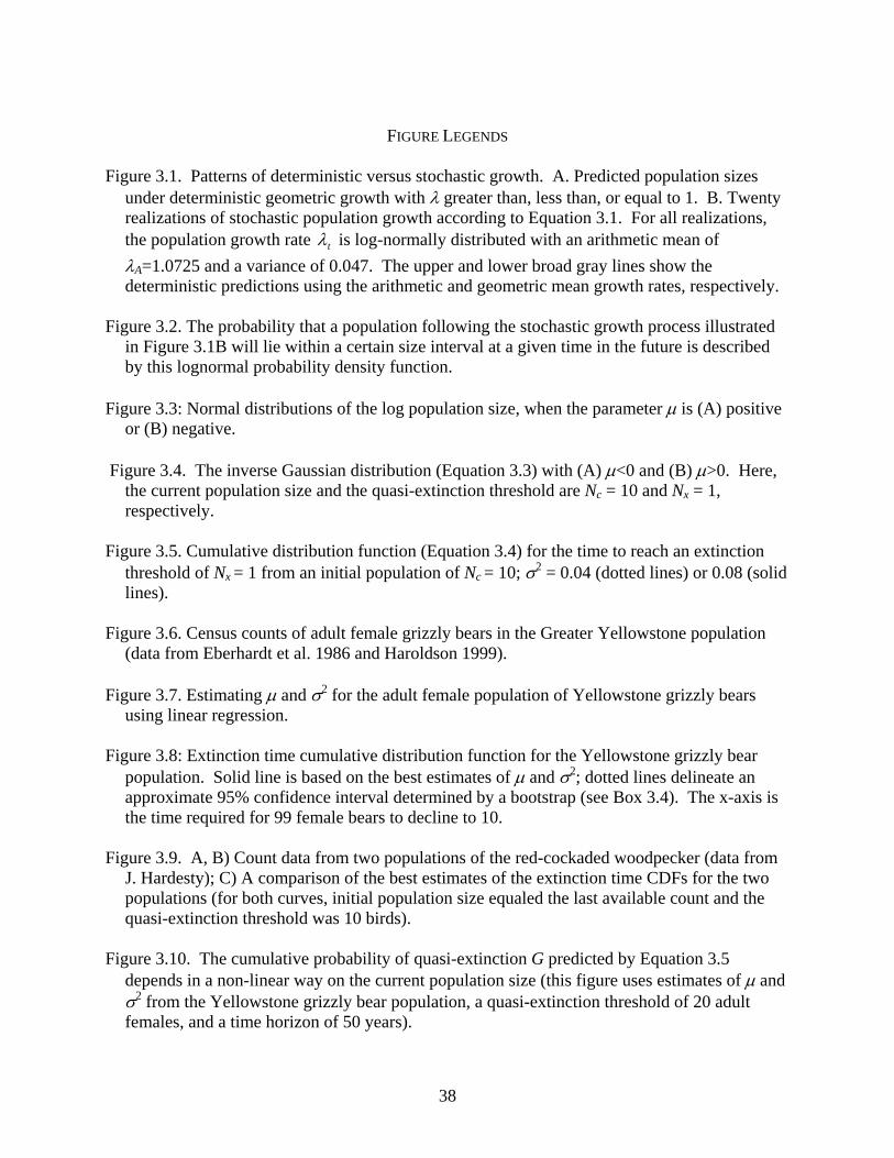
FIGURE LEGENDS

Figure 3.1. Patterns of deterministic versus stochastic growth. A. Predicted population sizes

under deterministic geometric growth with λ greater than, less than, or equal to 1. B. Twenty realizations of stochastic population growth according to Equation 3.1. For all realizations, the population growth rate tλ is log-normally distributed with an arithmetic mean of λA=1.0725 and a variance of 0.047. The upper and lower broad gray lines show the deterministic predictions using the arithmetic and geometric mean growth rates, respectively.

Figure 3.2. The probability that a population following the stochastic growth process illustrated

in Figure 3.1B will lie within a certain size interval at a given time in the future is described by this lognormal probability density function.

Figure 3.3: Normal distributions of the log population size, when the parameter µ is (A) positive

or (B) negative. Figure 3.4. The inverse Gaussian distribution (Equation 3.3) with (A) µ<0 and (B) µ>0. Here,

the current population size and the quasi-extinction threshold are Nc = 10 and Nx = 1, respectively.

Figure 3.5. Cumulative distribution function (Equation 3.4) for the time to reach an extinction

threshold of Nx = 1 from an initial population of Nc = 10; σ2 = 0.04 (dotted lines) or 0.08 (solid lines).

Figure 3.6. Census counts of adult female grizzly bears in the Greater Yellowstone population

(data from Eberhardt et al. 1986 and Haroldson 1999). Figure 3.7. Estimating µ and σ2 for the adult female population of Yellowstone grizzly bears

using linear regression. Figure 3.8: Extinction time cumulative distribution function for the Yellowstone grizzly bear

population. Solid line is based on the best estimates of µ and σ2; dotted lines delineate an approximate 95% confidence interval determined by a bootstrap (see Box 3.4). The x-axis is the time required for 99 female bears to decline to 10.

Figure 3.9. A, B) Count data from two populations of the red-cockaded woodpecker (data from

J. Hardesty); C) A comparison of the best estimates of the extinction time CDFs for the two populations (for both curves, initial population size equaled the last available count and the quasi-extinction threshold was 10 birds).

Figure 3.10. The cumulative probability of quasi-extinction G predicted by Equation 3.5

depends in a non-linear way on the current population size (this figure uses estimates of µ and σ2 from the Yellowstone grizzly bear population, a quasi-extinction threshold of 20 adult females, and a time horizon of 50 years).

38

Figure 3.11. The annual log growth rates for the Yellowstone grizzly bear population do not show any obvious signs of density dependence.

39

Fig. 3.1

0

5

10

15

20

25

30

0 5 10 15 20

Year, t

Popu

latio

n siz

e, N

t A 05.1=λ

1=λ

95.0=λ

0

20

40

60

80

100

120

140

0 5 10 15 20Year, t

Popu

latio

n siz

e, N

t

B

λ

λG

A

Fig. 3.2

0

0.005

0.01

0.015

0.02

0.025

0.03

0.035

0.04

0.045

0.05

0 25 50 75 100 125 150

Population size, N t

Prob

abili

ty d

ensi

ty

t =10

t =20

t =30

t =40

t =50

Fig. 3.3

ALog N(t)

Initial Population

Size

µ>0Variance

= σ2tNormalDistribution

Log N0

Mean=µt

tt 2 t3t 1

Log N(t) µ<0 BLog N0

tt 2 t3t 1

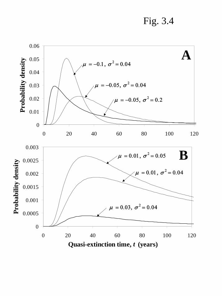
Fig. 3.4

0

0.0005

0.001

0.0015

0.002

0.0025

0.003

0 20 40 60 80 100 120

Quasi-extinction time, t (years)

Prob

abili

ty d

ensi

ty

µ = 0.01, σ 2 = 0.04

µ = 0.01, σ 2 = 0.05

µ = 0.03, σ 2 = 0.04

B

0

0.01

0.02

0.03

0.04

0.05

0.06

0 20 40 60 80 100 120

Prob

abili

ty d

ensi

ty

µ = −0.05, σ 2 = 0.04

µ = −0.1, σ 2 = 0.04

µ = −0.05, σ 2 = 0.2

A

Fig. 3.5

00.10.20.30.40.50.60.70.80.9

1

0 10 20 30 40 50Time horizon, T (years)

Prob

abili

ty e

xtin

ctio

n th

resh

old

is r

each

ed

befo

re ti

me

T

µ = -0.1

µ = -0.05

µ = 0.01

Fig. 3.6

30

40

50

60

70

80

90

100

58 60 62 64 66 68 70 72 74 76 78 80 82 84 86 88 90 92 94 96 98Year

Adu

lt Fe

mal

es

Yellowstone Grizzly Bear

Fig. 3.7

-0.3

-0.2

-0.1

0.0

0.1

0.2

0.3

0 0.2 0.4 0.6 0.8 1 1.2

Slope = µ

Residual mean square = σ 2

Zerointercept

(t i+ 1 - t i )1/2

log(

Ni+

1/Ni)

/(ti+

1-t i

)1/2

Figure 3.8

0 5 10 15 20 25 30 35 40 45 50

10-15

10-10

10-5

100

Years into the future

Cum

ulat

ive

prob

abili

ty o

f qua

si-e

xtin

ctio

n

Central Florida Red-Cockaded Woodpecker

010203040506070

80 82 84 86 88 90 92

Year

Adu

lt B

irds

Extinction Time CDF

00.10.20.30.40.50.60.70.80.9

1

0 100 200 300 400 500Time (years)

Cum

ulat

ive

Prob

abili

ty

North Carolina Red-Cockaded Woodpecker

380400

420440

460

480

80 85 90 95Year

Adu

lt B

irds

Central Florida

North Carolina

A

B

C

Fig. 3.9

Figure 3.10

20 30 40 50 60 70 80 90 1000

0.1

0.2

0.3

0.4

0.5

0.6

0.7

0.8

0.9

1

Current population size

Prob

abili

ty o

f qua

si-e

xtin

ctio

n by

yea

r 50

Figure 3.11

-0.3

-0.2

-0.1

0

0.1

0.2

0.3

20 40 60 80 100

Numbers of Females in year t, Nt

log(

Nt+

1/Nt)