Chapter Nine

Radiation

Heinrich Rudolf Hertz

(1857 - 1894)

October 12, 2001

Contents

1 Introduction 1

2 Radiation by a localized source 3

2.1 The Near Zone . . . . . . . . . . . . . . . . . . . . . . . . . . . . . . 6

2.2 The Radiation or Far Zone . . . . . . . . . . . . . . . . . . . . . . . . 6

3 Multipole Expansion of the Radiation Field 9

3.1 Electric Dipole . . . . . . . . . . . . . . . . . . . . . . . . . . . . . . 10

3.1.1 Example: Linear Center-Fed Antenna . . . . . . . . . . . . . . 13

3.2 Magnetic Dipole . . . . . . . . . . . . . . . . . . . . . . . . . . . . . . 14

3.3 Comparison of Dipoles . . . . . . . . . . . . . . . . . . . . . . . . . . 16

3.4 Electric Quadrupole . . . . . . . . . . . . . . . . . . . . . . . . . . . 18

3.4.1 Example: Oscillating Charged Spheroid . . . . . . . . . . . . . 21

3.5 Large Radiating Systems . . . . . . . . . . . . . . . . . . . . . . . . . 23

3.5.1 Example: Linear Array of Dipoles . . . . . . . . . . . . . . . . 24

1

4 Multipole expansion of sources in waveguides 26

4.1 Electric Dipole . . . . . . . . . . . . . . . . . . . . . . . . . . . . . . 26

5 Scattering of Radiation 31

5.1 Scattering of Polarized Light from an Electron . . . . . . . . . . . . . 31

5.2 Scattering of Unpolarized Light from an Electron . . . . . . . . . . . 34

5.3 Elastic Scattering From a Molecule . . . . . . . . . . . . . . . . . . . 35

5.3.1 Example: Scattering Off a Hard Sphere . . . . . . . . . . . . . 38

5.3.2 Example: A Collection of Molecules . . . . . . . . . . . . . . . 40

6 Diffraction 43

6.1 Scalar Diffraction Theory: Kirchoff Approximation . . . . . . . . . . 45

6.2 Babinet’s Principle . . . . . . . . . . . . . . . . . . . . . . . . . . . . 51

6.3 Fresnel and Fraunhofer Limits . . . . . . . . . . . . . . . . . . . . . 53

7 Example Problems 55

7.1 Example: Diffraction from a Rectangular Aperture . . . . . . . . . . 55

7.2 Example: Diffraction from a Circular Aperture . . . . . . . . . . . . . 57

7.3 Diffraction from a Cross . . . . . . . . . . . . . . . . . . . . . . . . . 60

7.4 Radiation from a Reciprocating Disk . . . . . . . . . . . . . . . . . . 61

1 Introduction

An electromagnetic wave, or electromagnetic radiation, has as its sources electric

accelerated charges in motion. We have learned a great deal about waves but have

not given much thought to the connection between the waves and the sources that

produce them. That oversight will be rectified in this chapter.

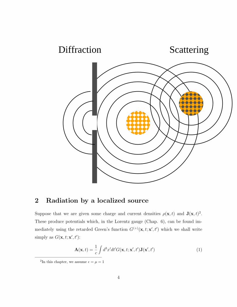
The scattering of electromagnetic waves is produced by bombarding some object

(the scatterer) with an electromagnetic wave. Under the influence of the fields in that

2

wave, charges in the scatterer will be set into some sort of coherent motion1 and these

moving charges will produce radiation, called the scattered wave. Hence scattering

phenomena are closely related to radiation phenomena.

Diffraction of electromagnetic waves is similar. One starts with a wave incident

on an opaque screen with holes, or aperture, in it. Charges in the screen, especially

around the apertures, are set in motion and produce radiation which in this case is

called the diffracted wave.

Thus radiation, scattering, and diffraction are closely related. We shall start

our investigation by considering the radiation produced by some specified localized

distribution of charges and currents in harmonic motion. We delay until Chap. 14,

the discussion of non-harmonic sources.

1The response to a harmonic excitation is of the same frequency, and thus coherent

3

Diffraction Scattering

2 Radiation by a localized source

Suppose that we are given some charge and current densities ρ(x, t) and J(x, t)2.

These produce potentials which, in the Lorentz gauge (Chap. 6), can be found im-

mediately using the retarded Green’s function G(+)(x, t; x′, t′) which we shall write

simply as G(x, t; x′, t′):

A(x, t) =1

c

∫d3x′dt′G(x, t; x′, t′)J(x′, t′) (1)

2In this chapter, we assume ε = µ = 1

4

Φ(x, t) =∫d3x′dt′G(x, t; x′, t′)ρ(x′, t′). (2)

The Green’s function itself is given by

G(x, t; x′, t′) =δ(t− t′ − |x− x′|/c)

|x− x′| . (3)

Because all of the equations we shall use to compute fields are linear in the fields

themselves, we may conveniently treat just one Fourier component (frequency) of the

field at a time. To this end we write

J(x, t) =1

2

∫ ∞

−∞dωJ(x, ω)e−iωt (4)

where

J(x,−ω) = J∗(x, ω) (5)

is required in order that J(x, t) be real; Eq. (5) is known as a “reality condition.” We

may equally well, and more conveniently, replace Eqs. (4) and (5) by

J(x, t) = <∫ ∞

0dωJ(x, ω)e−iωt. (6)

We will do this and will in general not bother to write < in front of every complex

expression whose real part must be taken. We will just have to remember that the

real part is the physically meaningful quantity. Similarly, we introduce the Fourier

transform of the charge density,

ρ(x, t) =∫ ∞

0dωρ(x, ω)e−iωt. (7)

In the following we shall suppose that the sources have just a single frequency

component,

J(x, ω′) = J(x)δ(ω − ω′), ω′ > 0 (8)

ρ(x, ω′) = ρ(x)δ(ω − ω′), ω′ > 0. (9)

Thus, assuming ω > 0,

J(x, t) = J(x)e−iωt and (10)

ρ(x, t) = ρ(x)e−iωt. (11)

5

From the continuity condition on the sources,

∂ρ(x, t)

∂t+∇ · J(x, t) = 0, (12)

we find that ρ(x) and J(x) are related by

ρ(x) = −i∇ · J(x)

ω. (13)

Using Eq. (10) in Eq. (1) and employing Eq. (3) for the Green’s function, we find,

upon completing the integration over the time, that

A(x, t) =1

c

∫d3x′

J(x′)

|x− x′|eik|x−x′|e−iωt (14)

where, as usual, k ≡ ω/c. Define A(x) by

A(x, t) = A(x)e−iωt; (15)

comparison with Eq. (14) gives

A(x) =1

c

∫d3x′ J(x′)

eik|x−x′|

|x− x′| . (16)

From here the recipe is to find B(x, t) from the curl of A(x, t); then the electric field

is found3 from ∇×B(x, t) = c−1∂E(x, t)/∂t, which holds in regions where the current

density vanishes. These fields have the forms

B(x, t) = B(x)e−iωt E(x, t) = E(x)e−iωt (17)

where

B(x) = ∇×A(x) E(x) =i

k∇×B(x). (18)

We have reduced everything to a set of straightforward calculations - integrals

and derivatives. Doing them exactly can be tedious, so we should spend some time

3Notice that we never have to evaluate the scalar potential.

6

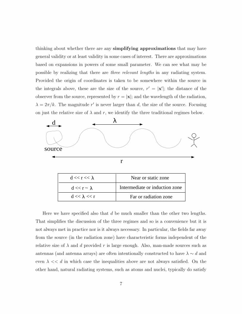
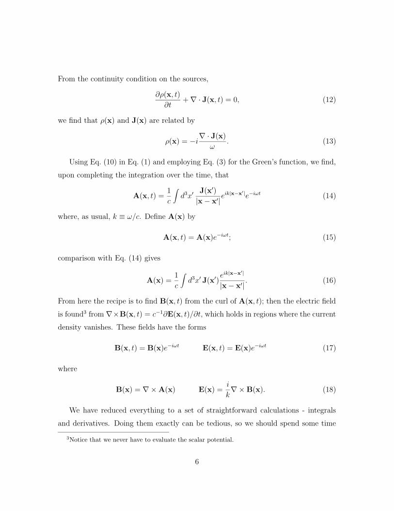
thinking about whether there are any simplifying approximations that may have

general validity or at least validity in some cases of interest. There are approximations

based on expansions in powers of some small parameter. We can see what may be

possible by realizing that there are three relevant lengths in any radiating system.

Provided the origin of coordinates is taken to be somewhere within the source in

the integrals above, these are the size of the source, r′ = |x′|; the distance of the

observer from the source, represented by r = |x|; and the wavelength of the radiation,

λ = 2π/k. The magnitude r′ is never larger than d, the size of the source. Focusing

on just the relative size of λ and r, we identify the three traditional regimes below.

source

λ

r

d

d << r << λ

d << r ~ λd << λ << r

Near or static zone

Intermediate or induction zone

Far or radiation zone

Here we have specified also that d be much smaller than the other two lengths.

That simplifies the discussion of the three regimes and so is a convenience but it is

not always met in practice nor is it always necessary. In particular, the fields far away

from the source (in the radiation zone) have characteristic forms independent of the

relative size of λ and d provided r is large enough. Also, man-made sources such as

antennas (and antenna arrays) are often intentionally constructed to have λ ∼ d and

even λ << d in which case the inequalities above are not always satisfied. On the

other hand, natural radiating systems, such as atoms and nuclei, typically do satisfy

7

the condition d << λ and d << r for any r at which it is practical to detect the

radiation.

2.1 The Near Zone

Consider first the near zone. Here d << λ and r << λ, so there is a simple expansion

of the exponential factor,

eik|x−x′| = 1 + ik|x− x′|+ ... (19)

which leads to

A(x, t) =1

c

∫d3x′

J(x′)

|x− x′| [1 + ik|x− x′|+ ...]e−iωt. (20)

The leading term in this expansion is

A(x, t) =1

c

∫d3x′

J(x′)

|x− x′|e−iωt. (21)

Aside from the harmonic time dependence, this is just the vector potential of a static

current distribution J(x), and that is the origin of the name “static” zone; the mag-

netic induction here has a spatial dependence which is the same as what one would

find for a static current distribution with the spatial dependence of the actual oscil-

lating current distribution. We find this result for the simple reason that in the near

zone the exponential factor can be approximated as unity.

2.2 The Radiation or Far Zone

In the radiation or far zone (r À λÀ d), the story is completely different because

in this regime the behavior of the exponential dominates the integral. We can most

easily see what will happen if we first expand the displacement |x− x′| in powers of

r′/r (d/r):

|x− x′| = [(x− x′) · (x− x′)]1/2 = (r2 − 2x · x′ + r′2)1/2

= r

1− 2x · x′

r2+

(r′

r

)2

1/2

= r

1− 2

n · x′r

+

(r′

r

)2

1/2

(22)

8

where n = x/r is a unit vector in the direction of x. Carrying the expansion to second

order in r′/r, we have

|x− x′| = r

1− n · x′

r+

1

2

(r′

r

)2

− 1

2

(n · x′r

)2 . (23)

Similarly,

1

|x− x′| =1

r

1 +

n · x′r

+1

2

(r′

r

)23

(n · x′r′

)2

− 1

. (24)

Using the first of these expansions we can write

eik|x−x′| = eikre−ik(n·x′)ei kr

2

[(r′r

)2

−(

n·x′r

)2]

= eikre−ik(n·x′)ei kr′2

2r

[1− (n·x′)2

r′2

]. (25)

Given r >> r′ and kr′2/r << 1, it is clear that this exponential function can be

approximated by just the first two factors; the third represents a change of phase by

an amount small compared to a radian. Further, in the far zone it is sufficient to

approximate1

|x− x′| =1

r. (26)

Putting these pieces together we have

A(x, t) =ei(kr−ωt)

cr

∫d3x′ J(x′)e−ik(n·x′) (r À d and r À d2/λ) . (27)

This expression is always valid for r “large enough” which means r >> r′ and r >>

kr′2. The relative size of λ and d is unimportant.

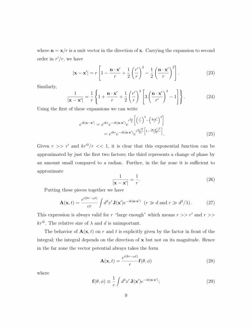
The behavior of A(x, t) on r and t is explicitly given by the factor in front of the

integral; the integral depends on the direction of x but not on its magnitude. Hence

in the far zone the vector potential always takes the form

A(x, t) =ei(kr−ωt)

rf(θ, φ) (28)

where

f(θ, φ) ≡ 1

c

∫d3x′ J(x′)e−ik(n·x′); (29)

9

θ and φ specify, in polar coordinates, the direction of x (or n).

Knowing the form of the potential so precisely makes it easy to see what must be

the form of the fields E and B in the far zone. First,

B(x, t) = ∇×A(x, t) = ∇×(ei(kr−ωt)

rf(θ, φ)

)≈ ik

ei(kr−ωt)

r[n× f(θ, φ)] (30)

where we have discarded terms of relative order λ/r or d/r. Further, from Eqs. (18)

and (30), we can find E(x,t); to the same order as B, it is

E(x, t) = −ik ei(kr−ωt)

r[n× (n× f(θ, φ))] = B(x, t)× n. (31)

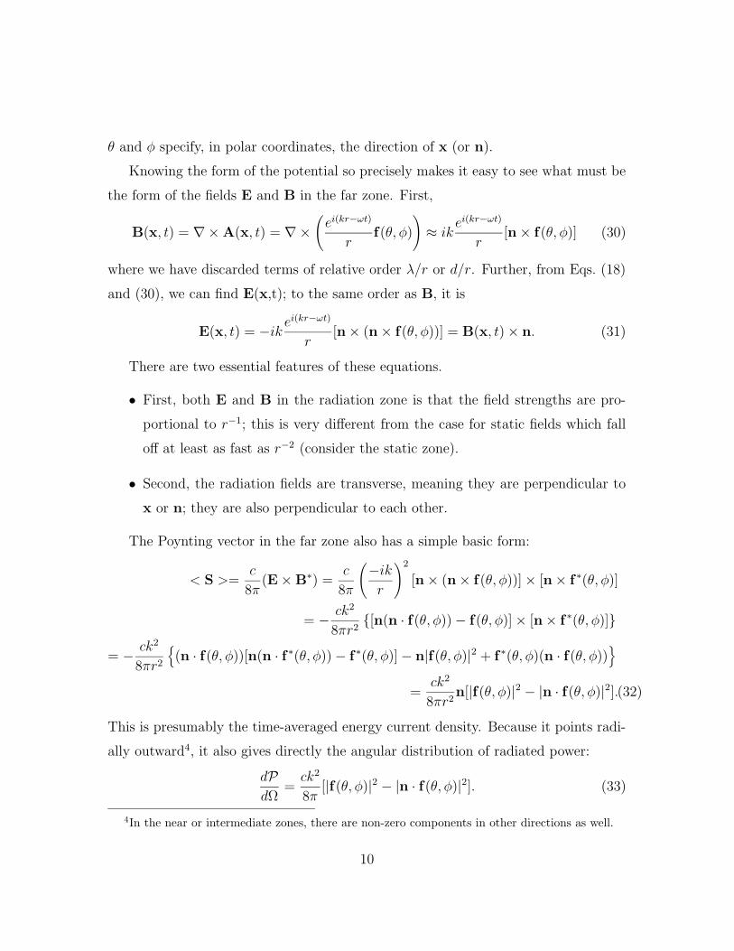
There are two essential features of these equations.

• First, both E and B in the radiation zone is that the field strengths are pro-

portional to r−1; this is very different from the case for static fields which fall

off at least as fast as r−2 (consider the static zone).

• Second, the radiation fields are transverse, meaning they are perpendicular to

x or n; they are also perpendicular to each other.

The Poynting vector in the far zone also has a simple basic form:

< S >=c

8π(E×B∗) =

c

8π

(−ikr

)2

[n× (n× f(θ, φ))]× [n× f ∗(θ, φ)]

= − ck2

8πr2[n(n · f(θ, φ))− f(θ, φ)]× [n× f ∗(θ, φ)]

= − ck2

8πr2

(n · f(θ, φ))[n(n · f ∗(θ, φ))− f ∗(θ, φ)]− n|f(θ, φ)|2 + f∗(θ, φ)(n · f(θ, φ))

=ck2

8πr2n[|f(θ, φ)|2 − |n · f(θ, φ)|2].(32)

This is presumably the time-averaged energy current density. Because it points radi-

ally outward4, it also gives directly the angular distribution of radiated power:

dPdΩ

=ck2

8π[|f(θ, φ)|2 − |n · f(θ, φ)|2]. (33)

4In the near or intermediate zones, there are non-zero components in other directions as well.

10

If we integrate over the solid angle, we find the total power radiated:

P =∮

Sd2x < S > ·n =

ck2

8π

∫dΩ [|f(θ, φ)|2 − |n · f(θ, φ)|2]. (34)

Notice that the radiated power is, appropriately, independent of r.

3 Multipole Expansion of the Radiation Field

Thus far, we have only assumed that r À λ, d. Now we will consider the d/λ.

Consider two limits:

• If d/λ ¿ 1, then all elements of the source will essentially be in phase, and

thus an observer at r cannot learn about the structure of the source from the

emitted radiation. In this limit, we need only consider the first finite moment

in d/λ (if the series is convergent).

• If d/λ >∼ 1, then the elements of the source will not radiate in phase, and an

observer at r may learn about the details of the structure of the source by

analyzing the interference of the radiation pattern (i.e. Bragg diffraction). In

this case, to be discussed in sec. V, we need to retain more terms in the series.

Let us now go back and attempt to evaluate f(θ, φ). If kd << 1, or 2πd/λ << 1,

then it is not unreasonable to proceed with the evaluation by expanding the expo-

nential function e−ik(n·x′),

f(θ, φ) =1

c

∫d3x′ J(x′)

[1− ik(n · x′)− 1

2k2(n · x′)2 + ...

]. (35)

3.1 Electric Dipole

The first term in the expansion is just the volume integral of J(x′); one can write it

as1

c

∫d3x′ J(x′) = −1

c

∫d3x′ [∇′ · J(x′)]x′ (36)

11

which one can show by doing integration by parts starting from the right-hand side

of this equation. Now employ Eq. (13) to have

1

c

∫d3x′ J(x′) = −ik

∫d3x′ x′ρ(x′). (37)

The right-hand side can be recognized as the electric dipole moment of the amplitude

ρ(x) of the harmonically varying charge distribution. Let us define the electric dipole

moment p in the usual way,

p ≡∫d3x′ x′ρ(x′). (38)

The electric dipole contribution fed(θ, φ) to f(θ, φ) is thus

fed(θ, φ) = −ikp; (39)

it is in fact independent of θ and φ. The corresponding contribution to the vector

potential, Aed(x, t), is

Aed(x, t) = −ikpei(kr−ωt)

r. (40)

We have used only d << λ and d << r; no assumption about the relative size

of λ and r has been made. It is somewhat tedious, but nevertheless instructive, to

evaluate the fields without making any assumptions so that we can see their form in

the near, intermediate, and far zones. First, the magnetic induction is

Bed(x) = ∇×Aed(x) = −ik∇(eikr

r

)× p

= −ik(ik − 1

r

)eikr

r(n× p) = k2

(1− 1

ikr

)eikr

r(n× p). (41)

Further, the electric field is

Eed(x) =i

k(∇×Bed(x))

= ik∇[eikr

r

(1− 1

ikr

)]× (n× p) + ik

eikr

r

(1− 1

ikr

)∇× (n× p)

= ik

(ik

r− 1

r2

)(1− 1

ikr

)+

1

ikr3

eikrn× (n× p)

12

+ikeikr

r

(1− 1

ikr

) [(p · ∇)

(x

r

)− p∇ ·

(x

r

)]

=k2

r

[−1 +

2

ikr+

2

k2r2

]eikrn× (n× p)

+ik

reikr

(1− 1

ikr

)(p

r− (p · n)n

r− 3p

r+

p

r

)

=

−k

2

rn× (n× p) +

1

r3(1− ikr)[3n(p · n)− p]

eikr. (42)

The electric field is divided up in this fashion to bring out, first, the form in the

radiation zone which is the first term and, second, the form in the near zone r << λ

which is the second term. The spatial dependence of the latter is the same as the field

of a static dipole, [3n(p · n)− p]/r3, but do not forget that it oscillates with angular

frequency ω. In the intermediate zone where all contributions are comparable, the

field is complex indeed.5

In the radiation zone, where the fields become quite simple, they are

Bed(x) =k2

reikr(n× p) and Eed = −k

2

reikrn× (n× p). (43)

The same conclusion may be reached much more simply from Eqs. (30), (31), and (39).

As remarked earlier, the fields in the far zone are transverse to n. If we let p define

the polar axis, then Bed is azimuthal, i.e., in the direction of φ. This is a special

feature of electric dipole radiation. Further, Eed(x) is in the direction of θ.

p r

SE

B

5And this is only the electric dipole part of the field which is, along with the magnetic dipole

part of the field, by far the simplest.

13

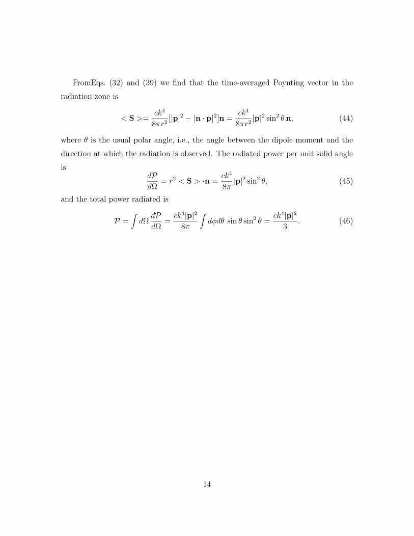
FromEqs. (32) and (39) we find that the time-averaged Poynting vector in the

radiation zone is

< S >=ck4

8πr2[|p|2 − |n · p|2]n =

ck4

8πr2|p|2 sin2 θ n, (44)

where θ is the usual polar angle, i.e., the angle between the dipole moment and the

direction at which the radiation is observed. The radiated power per unit solid angle

isdPdΩ

= r2 < S > ·n =ck4

8π|p|2 sin2 θ, (45)

and the total power radiated is

P =∫dΩ

dPdΩ

=ck4|p|2

8π

∫dφdθ sin θ sin2 θ =

ck4|p|23

. (46)

14

3.1.1 Example: Linear Center-Fed Antenna

Consider the short, linear, “center-fed” antenna shown below.

d/2

-d/2

x

y

z

n

Fig. 1 Short, center-fed, linear antenna.

θ

For such an antenna, the current density can be crudely approximated by

J(x, t) = ε3I0δ(x)δ(y)

(1− 2

|z|d

)e−iωt (47)

for |z| < d/2; for |z| > d/2, it is zero. Given this current density, we can evaluate the

divergence and so find the charge density,

∇ · J(x) = −2I0

dδ(x)δ(y)

z

|z| = −iωρ(x) (48)

or

ρ(x) =2iI0

ωdδ(x)δ(y)

z

|z| , |z| < d/2. (49)

Hence,

p =∫d3xxρ(x) =

iI0d

2ckε3. (50)

15

Now we have only to plug Eq. (50) into Eqs. (45) and (46) to find

dPdΩ

=I2

0

32πc(kd)2 sin2 θ and P =

I20k

2d2

12c. (51)

The calculation in this example may be expected to provide a good approximation to

the total radiated power provided kd << 1 so that the electric dipole term dominates,

unless it vanishes. There are many instances where this happens.

3.2 Magnetic Dipole

When this happens it is necessary to look at higher-order terms in the expansion

of the phase factor eik|x−x′|. Let’s look now at the next one. Start from the exact

expression for A(x),

A(x) =1

c

∫d3x′ J(x′)

eik|x−x′|

|x− x′|

= Aed(x) +eikr

cr

∫d3x′ J(x′)

(n · x′r− ik(n · x′)

)[1 +O(d/r, d/λ)]. (52)

where the second term in the () comes from the exponential, and the first comes from

the corresponding denominator. The integral we wish to examine is

1

c

∫d3x′ J(x′)(n · x′)

=1

2c

∫d3x′ [J(x′)(n · x′) + x′(n · J(x′))] + [J(x′)(n · x′)− x′(n · J(x′))]

=1

2c

∫d3x′ [J(x′)(n · x′) + x′(n · J(x′))] +

1

2c

∫d3x′ n× (J(x′)× x′) (53)

What is the point of breaking the integral into two pieces, symmetric and antisym-

metric under interchange of x′ and J(x′)? There are several related points. One is

that in the near zone the second term on the right-hand side produces a magnetic

induction which has the form of the induction of a static magnetic dipole while the

first term produces an electric field which has the form of the field of a static electric

quadrupole. Hence the radiation from the former is called magnetic dipole radia-

tion while that from the latter is known as electric quadrupole radiation. Also, the

16

magnetic dipole part produces a purely transverse electric field in all zones while the

electric quadrupole part gives a purely transverse magnetic induction. Recall that for

electric dipole radiation, B(x, t) is purely transverse in all zones as well.

Let us look at the magnetic dipole fields first. From Eqs. (52) and (53) we have

Amd(x) =eikr

r

(1

r− ik

)n×

∫d3x′

1

2c(J(x′)× x′)

≡ −ik eikr

r

(1− 1

ikr

)(n×m) (54)

where

m ≡ 1

2c

∫d3x′ [x′ × J(x′)] (55)

is the magnetic dipole moment, familiar from our study of magnetostatics.

Rather than plow ahead with with the evaluation of the curl to find B, etc., let

us recall the electric dipole results

Aed(x) = −ik eikr

rp (56)

Bed(x) = k2 eikr

r

(1− 1

ikr

)(n× p). (57)

We see that Bed is the same in functional form as Amd; consequently, Eed, which is

the curl of Bed, must be the same in form as the curl of Amd, or Bmd. Hence we can

immediately write, using Eq. (43),

Bmd(x) = k2 eikr

rn× (n×m) +

eikr

r3(1− ikr)[3n(n ·m)−m]. (58)

Notice that in the near zone Bmd(x) is the same as that of a static dipole.

As for the corresponding electric field, we could work through the tedious deriva-

tives of the magnetic induction, but it happens that this is one time when it is much

easier to evaluate the the field from the potentials. We know that

E(x, t) = −∇Φ(x, t)− 1

c

∂A(x, t)

∂t. (59)

17

Also, in the Lorentz gauge

∇ ·A(x, t) +1

c

∂Φ(x, t)

∂t= 0 or ∇ ·A(x)− ikΦ(x) = 0. (60)

Using this relation for Φ(x), we find that

E(x) = − ik∇(∇ ·A(x)) + ikA(x) (61)

for any electric field which is harmonic in time. From our expression for Amd(x), one

can easily see that ∇ · Amd = 06 and so Emd is simply proportional to the vector

potential,

Emd(x) = −k2 eikr

r

(1− 1

ikr

)(n×m). (62)

3.3 Comparison of Dipoles

To summarize:

• The electric dipole and magnetic dipole fields are the same with E and B

interchanged, Emd ⇔ −Bed and Bmd ⇔ Eed when p⇔m.

• In the near zone Eed and Bmd have the form of static dipole fields, while in all

zones, Bed and Emd are purely azimuthal in direction.

• The Poynting vector in the far zone has the same form for both electric dipole

and magnetic dipole fields; in the latter case it is

< S >= r2nck4

8π|m|2 sin2 θ, (63)

leading to results for the power distribution and total power which are the same

as for electric dipole radiation, Eqs. (45) and (46), with m in place of p. Notice

particularly that if one measures dP/dΩ, and finds the sin2 θ pattern, then one

6An equivalent statement is that a magnetic dipole is always charge neutral, so that Φ = 0.

18

knows that the radiation is indeed7 dipole radiation; however, it is impossible

to distinguish electric dipole radiation from magnetic dipole radiation without

examining its polarization.

Magnetic DipoleElectric Dipole

mx = r n

p

x = r n E

BE

B

)(i kr

/ rn x m=k e2

EBE = -n x B B = n x E

p m

B - EE B

= -k e (2 i kr

) / rn x mp

These formulas suggest that for a given set of moving charges, one should get as

much power out of an oscillating magnetic dipole as an oscillating electric dipole.

This is not so, since the magnetic dipole moment is

m ≡ 1

2c

∫d3x′ [x′ × J(x′)] (64)

thus

|m| ∼ v

cQd (65)

where v is the speed of the moving charge, Q is the magnitude of this charge, and d

is the size of the current loop. The size of the corresponding electric dipole moment

7Higher-order multipoles produce radiation with distinctive angular distributions which are never

proportional to sin2 θ.

19

is roughly Qd. Thus,

|m| ∼ v

c|p| (66)

We see that

Pmd ≈(v

c

)2

Ped . (67)

Thus, in a system with both an electric and magnetic dipole moment, the latter is

usually a relativistic correction to the former.

3.4 Electric Quadrupole

Let’s go now to the other contribution to the vector potential in Eq. (53). This is

called the electric quadrupole term; knowing that, we naturally expect to find that

it produces an electric field in the near zone which has the characteristic form of a

static electric quadrupole field. The vector potential is

Aeq(x) =eikr

r

(1

r− ik

)1

2c

∫d3x′ [J(x′)(n · x′) + x′(n · J(x′))]

= −eikr

r

(1

r− ik

)1

2c

∫d3x′ (n · x′)(∇′ · J(x′))x′. (68)

To demonstrate this algebraic step, consider the ith component of the final expression:

1

2c

∫d3x′ (n · x′)

∑

j

∂Jj∂x′j

x′i = − 1

2c

∑

j

∫d3x′

∂

∂x′j[x′i(n · x′)]Jj

= − 1

2c

∫d3x′

∑

j

[δij(n · x′) + x′inj]Jj

= − 1

2c

∫d3x′ [Ji(n · x′) + x′i(n · J)] (69)

which matches the ith component of the original expression in Eq. (68). Making use

of Eq. (13) for ∇ · J(x) and also using ω = ck, we find, from Eq. (68), that

Aeq(x) = −k2

2

eikr

r

(1− 1

ikr

) ∫d3x′ x′(n · x′)ρ(x′). (70)

20

There are nine components to the integral since the factor of n in the integrand can

be used to project out three numbers by, for example, letting n be each of the Carte-

sian basis vectors. That is, the basic integral over the source, ρ(x), which appears

here is a dyadic,∫d3xxxρ(x). It is symmetric and so has at most six independent

components. Notice also that Aeq depends on the direction of n, which was not the

case for either Aed or Amd; the evaluation of the fields is further complicated as a

consequence.

The electric quadrupole vector potential can be written in terms of the components

Qij of the electric quadrupole moment tensor which we defined long ago. Recall that

Qij ≡∫d3x (3xixj − r2δij)ρ(x). (71)

Take combinations of these to construct the components Qi of a vector Q:

Qi(n) ≡3∑

j=1

Qijnj. (72)

From these definitions one can show quite easily that

1

3n×Q(n) ≡ n×

(∫d3x′ x′(n · x′)ρ(x′)

). (73)

To see this, note that the ith component of Q/3 is

1

3Qi =

∫d3x′ [x′i(

∑

j

njx′j)ρ(x′)− r′2niρ(x′)/3]. (74)

The first term on the right-hand side of this relation produces the ith component of

the integral in Eq. (73); the second term is some i-independent quantity multiplied

by ni; the three terms in Q of this form give something which is directly proportional

to n and so they do not contribute to n×Q.

Thus have we established the validity of Eq. (73). But what good is it? It tells

us that we can write n×Aeq in terms of n×Q, but does not allow us to write Aeq

itself in terms of Q. However, if we restrict our attention to the radiation zone, then

21

n × A is all we will need, because in this zone, B = ik(n × A) and E = −n × B.

Thus, in the far zone,

Beq(x) = − ik3

6

eikr

r[n×Q(n)] (75)

and

Eeq(x) =ik3

6

eikr

rn× [n×Q(n)]. (76)

The time-averaged power radiated is

dPdΩ

= r2 < S · n > =c

8πr2[E(x)×B∗(x)] · n =

c

8πr2[B∗(x)× n] · E(x)

=c

8π

k6

36|n× [n×Q(n)]|2 =

ck6

288π|n×Q(n)|2. (77)

The right-hand side does not have any single form as a function of θ and φ that we

can extract because Q(n) depends in an unknown way (in general) on these angles.

We can proceed to a general result only up to a point:

|n×Q|2 = (n×Q) · (n×Q∗) = [(n×Q)× n] ·Q∗

= −Q∗ · [n(Q · n)−Q] = |Q|2 − |n ·Q|2; (78)

this is a brilliant derivation of the statement that sin2 θ = 1− cos2 θ. Further,

Q ·Q∗ − (n ·Q)(n ·Q∗) =∑

ijk

QijnjQ∗iknk −

∑

ijkl

niQijnjnkQ∗klnl. (79)

The ni’s are direction cosines and so obey the identities∫dΩninj =

4π

3δij (80)

and ∫dΩninjnknl =

4π

15(δijδkl + δikδjl + δilδjk). (81)

These enable us at least to get a simple result for the total radiated power:

P =∫dΩ

dPdΩ

=ck6

288π

4π

3

∑

ij

|Qij|2 −4π

15

∑

ik

[QiiQ∗kk + |Qik|2 +QijQ

∗ji]

=ck6

360

∑

ij

|Qij|2 (82)

22

where we have used the facts that Qij = Qji and∑iQii = 0.

By choosing appropriate axes (the principal axes of the quadrupole moment matrix

or tensor) one can always put the matrix of quadrupole moments into diagonal form.

Further, only two of the diagonal elements can be chosen independently because the

trace of the matrix must vanish. Hence any quadrupole moment matrix is a linear

combination of two basic ones.

3.4.1 Example: Oscillating Charged Spheroid

A commonly occurring example is an oscillating spheroidal charge distribution leading

to

Q33 = Q0 and Q22 = Q11 = −Q0/2. (83)

Then

Qi =∑

j

Qijnj = Qiini (84)

or

Q = Q0

[cos θε3 −

1

2sin θ(cosφ ε1 + sinφ ε2)

]. (85)

From this we have

|Q|2 = Q20

(cos2 θ +

1

4sin2 θ

),

n ·Q = Q0

(cos2 θ − 1

2sin2 θ

),

|n ·Q|2 = Q20

(cos4 θ − cos2 θ sin2 θ +

1

4sin4 θ

), (86)

and so

|Q|2 − |n ·Q|2 = Q20

[cos2 θ +

1

4sin2 θ − cos4 θ + sin2 θ cos2 θ − 1

4sin4 θ

]

= Q20

[cos2 θ sin2 θ +

1

4cos2 θ sin2 θ + cos2 θ sin2 θ

]

=9

4Q2

0 cos2 θ sin2 θ. (87)

23

Hence,dPdΩ

=ck6

128πQ2

0 sin2 θ cos2 θ. (88)

This is a typical, but not uniquely so, electric quadrupole radiation distribution.

dPdW

q

Radiation Pattern of an oscillating charged spheriodHigher-order multipole radiation (including magnetic quadrupole radiation) is

found by expanding the factor e−ik(n·x′) in Eq. (27) to higher order in powers of

d/λ. One can do this in a complete and systematic fashion after first developing

some appropriate mathematical machinery by generalizing the spherical harmonics

to vector fields,8 the purpose being to construct an orthonormal set of basis functions

for the electromagnetic fields.

8Thereby producing the so-called vector spherical harmonics. This is the subject matter of

Chapter 16.

24

3.5 Large Radiating Systems

Before abandoning the topic of simple radiating systems, let us look at one example

of an antenna which is not small compared the wavelength of the emitted radiation.

Our example is an array of antennas, each of which is itself small compared to λ and

each of which will be treated as a point dipole. We take the current density of this

array to be

J(x) = I0a∑

j

δ(x− xj)eiφjε3. (89)

One can easily see that this is an array of point antennas located at positions xj;

they all have the same current but are not necessarily in phase, the phase of the j th

antenna being given by φj (the additional phase factor e−iωt, common to all antennas,

has been omitted, as usual).

Antenna farmp

d << λD r >> D

No matter how large the array, we can specify that x is large enough that the

observation point is in the far zone in which case the vector potential can be taken

as

A(x) =eikr

rf(θ, φ) (90)

where

f(θ, φ) = ε3I0a

c

∫d3x′

∑

j

δ(x′ − xj)e−ik(n·x′)eiφj

= ε3I0a

c

∑

j

ei[φj−k(n·xj)]. (91)

Referring back to Eq. (33) we find that the distribution of radiated power is

dPdΩ

=k2I2

0a2

8πcsin2 θ|w|2 (92)

25

where

w ≡∑

j

ei(φj−kn·xj). (93)

The factor of sin2 θ arises because each element of this array is treated in the dipole

approximation. The factor |w|2 contains all of the information about the relative

phases of the amplitudes from the different elements, i.e., about the interference of

the waves from the different elements.

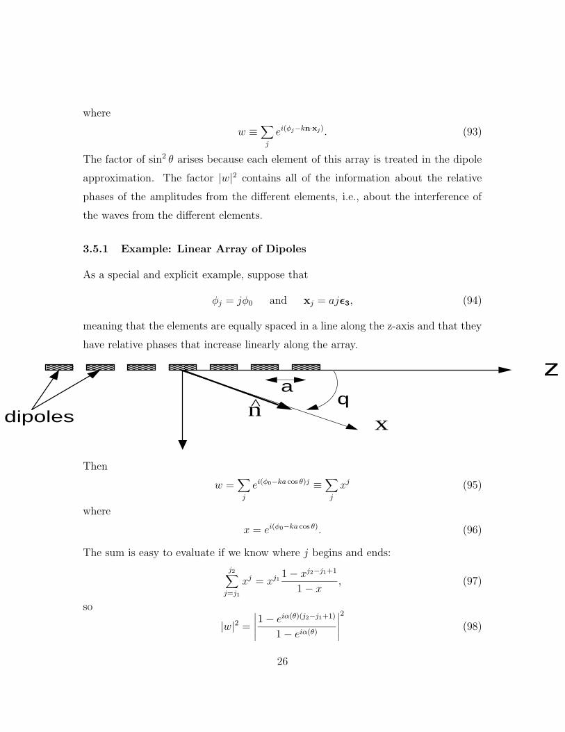
3.5.1 Example: Linear Array of Dipoles

As a special and explicit example, suppose that

φj = jφ0 and xj = ajε3, (94)

meaning that the elements are equally spaced in a line along the z-axis and that they

have relative phases that increase linearly along the array.

z

dipoles

aq

xn

Then

w =∑

j

ei(φ0−ka cos θ)j ≡∑

j

xj (95)

where

x = ei(φ0−ka cos θ). (96)

The sum is easy to evaluate if we know where j begins and ends:

j2∑

j=j1

xj = xj11− xj2−j1+1

1− x , (97)

so

|w|2 =

∣∣∣∣∣1− eiα(θ)(j2−j1+1)

1− eiα(θ)

∣∣∣∣∣

2

(98)

26

where α(θ) ≡ φ0 − ka cos θ. Let j1 = −n and j2 = n, corresponding to an array of

2n+ 1 elements centered at the origin. Then

|w|2 =

∣∣∣∣∣1− eiα(2n+1)

1− eiα∣∣∣∣∣

2

=1− cos[(2n+ 1)α]

1− cosα. (99)

This is a function which is in general of order unity and which oscillates as a function

of θ. It has, however, a large peak of size (2n+ 1)2 when α(θ) is an integral multiple

of 2π. The peak occurs at that angle θ0 where9 α(θ0) = 0 or cos θ0 = φ0/ka. If we

choose φ0 = 0, the peak is at θ0 = π/2; further, if ka < 2π or a < λ, there is no other

such peak. The width of the peak can be determined from the fact that the factor

w goes to zero when (2n + 1)α(θ) = 2π. Assuming that n >> 1, one finds that the

corresponding angle θ differs from θ0 by η where

η =2π

(2n+ 1)ka[1− (φ0/ka)2]∼ (2n+ 1)−1. (100)

Hence the antenna becomes increasingly directional with increasing n. The accompa-

nying figure shows the power distribution in units of k2I20a

2/8πc for 5 elements with

ka = π and φ0 = 0.

0 50 100 150-30

-10

10

30

dP/dΩ

9More generally, α(θ0) = 2mπ where m is an integer; because we control φ0, we can make it

small enough that the peak corresponds to the particular case m = 0.

27

4 Multipole expansion of sources in waveguides

We saw in Chapter 8 that a field in a waveguide could be expanded in the normal

modes of the waveguide with an integral over the sources, consisting of a current dis-

tribution and apertures, determining the coefficients in the expansion. If the sources

are small in size compared to distances over which fields in the normal modes vary,

then one can do the integrals in an approximate fashion by making a multipole ex-

pansion of the sources.

4.1 Electric Dipole

Consider first the part of the amplitude which is produced by some explicit current

distribution. It is

A(±)λ = −2πZλ

c

∫d3x′ J(x′) · E(∓)

λ . (101)

The field in the mode is given by

E(±)λ (x′) = [Eλ(x′, y′)± ε3Ezλ(x′, y′)]e±ikλz

′. (102)

The origin of the coordinate x′ is at some appropriately chosen point which is probably

not near the center of the source distribution. Let us use a different coordinate x

having as origin a point near the center of the source. Also, let’s let the electric

field in the mode be called E(x) as a matter of convenience. Then we have to do an

integral of the form

∫d3xJ(x) · E(x) =

∫d3xJ(x) ·

E(0) +

∑

i.j

∂Ei∂xj

∣∣∣∣∣0

εixj + ...

(103)

where we are assuming that the field varies little over the size of the source. In this

integral the first term can be converted to an integral over the charge density,

∫d3xJ(x) = −iω

∫d3xxρ(x) (104)

28

provided the integration by parts can be done without picking up a contribution

from the surface of the integration volume. That is not automatic here because the

surface includes some points on the wall of the waveguide including those points where

the current is fed into the guide, so one has to exercise some care in applying this

formula. Assuming that it is okay, we see that the leading term in the expansion

of the integrand produces to a term in the coefficient A(±)λ which is proportional to

p · E(0).

The next term in the expansion can, as we have seen, be divided into symmetric

and antisymmetric parts:

∑

i,j

∂Ei∂xj

∣∣∣∣∣0

∫d3x Ji(x)xj =

1

4

∑

i,j

(∂Ei∂xj− ∂Ej∂xi

)∣∣∣∣∣0

∫d3x [Jixj − Jjxi]

+1

2

∂Ei∂xj

∣∣∣∣∣0

∫d3x [Jixj + Jjxi]. (105)

The first term on the right-had side is set up in such a way as to display explicitly

a component of ∇× E, which is i(ω/c)B, and the same component of the magnetic

dipole moment. Hence this term is proportional to m · B(0). The remaining term

can be handled in the way that we treated the electric quadrupole part of the vector

potential earlier; it becomes

− iω2

∑

i,j

∂Ei∂xj

∣∣∣∣∣0

∫d3xxixjρ(x) = − iω

6

∑

i,j

Qij∂Ei∂xj

∣∣∣∣∣0

(106)

provided one can throw away the contributions that come from the surface when

the integration by parts is done. The final step is achieved by making use of the fact

that ∇ · E = 0.

In the next order, not shown in Eq. (103), the antisymmetric part provides the

magnetic quadrupole contribution. Without delving into the algebra of the derivation,

we state that the result is of the same form as Eq. (106) but with the magnetic

quadrupole moment tensor QMij in place of the electric quadrupole moment tensor, B

in place of E, and an overall relative (−). The components of the magnetic quadrupole

29

moment tensor are defined in the same way as those of the electric quadrupole moment

tensor except that in place of ρ(x) there is

ρM(x) = − 1

2c∇ · [x× J(x)]. (107)

The final result for the amplitude A(±)λ with all indices in place is

A(±)λ = i

2πω

c

p · E(∓)

λ (0)−m ·B(∓)λ +

1

6

∑

i,j

Qij

∂E(∓)iλ

∂xj

∣∣∣∣∣∣0

−QMij

∂B(∓)iλ

∂xj

∣∣∣∣∣∣0

+ ...

.

(108)

We can see immediately some interesting features of this result. For example, if

one wants to produce TM modes, which have z components of E but not of B, then

this is most efficiently done by designing the source to have a large pz. At the same

time, hardly any TE mode will be generated if there is only a z component of p

because the TE mode has no Ez to couple to p. Hence this expression gives one a

good idea how to design a source to produce, or not produce, modes of a given kind.

Now let’s look at the same expansion if the source of radiation is an aperture

rather than an explicit current distribution. We derived in chapter 8 that in this case

A(±)λ = −Zλ

2

∫

Sad2x′ n ·

[E(x′)×H

(∓)λ (x′)

]

= −Zλ2

∫

Sad2x′ [n× E(x′)] ·H(∓)

λ (x′) (109)

where the integral is over the aperture Sa, E(x′) is the electric field actually present

at point x′, and n is the inward directed normal at the aperture. Notice that only

the tangential component of the electric field contributes to this integral. Assuming

that the aperture is small compared to distances over which the fields in the normal

modes vary, we can expand the latter and find, after changing the origin to a point

in the aperture,

A(±)λ = −Zλ

2

∫

Sad2x (n× Etan) ·

H

(∓)λ (0) +

∑

i,j

εi∂H

(±)iλ

∂xj

∣∣∣∣∣∣0

xj + ...

= −Zλ2

B(∓)λ (0)

µ

∫

Sad2x (n× Etan) +

∑

i.j

∫

Sad2x (n× Etan)i

∂H(∓)iλ

∂xj

∣∣∣∣∣∣0

xj + ...

.(110)

30

The first term here has already an appropriate form. As for the second one, note that

we can break up the integrand into even and odd pieces,

(n× Etan)i∂Hiλ

∂xjxj =

1

2[(n× Etan)ixj − (n× Etan)jxi]

∂H(∓)iλ

∂xj

∣∣∣∣∣∣0

+1

2[(n× Etan)ixj + (n× Etan)jxi]

∂H(∓)iλ

∂xj

∣∣∣∣∣∣0

. (111)

Take just the antisymmetric part of this expression and complete the integral over x.

The contribution to the amplitude, aside from a factor of −Zλ/2, is

1

4

∑

i,j

∫

Sad2x[(n× Etan)ixj − (n× Etan)jxi]

∂H

(∓)iλ

∂xj− ∂H

(∓)jλ

∂xi

∣∣∣∣∣∣0

=1

4

∑

i,j,k

∫

Sad2x [(n× Etan)ixj − (n× Etan)jxi]εkij

(− iωε

cE

(∓)kλ (0)

)

= − iωε4c

∫

Sad2xE

(∓)λ (0) · [2x× (n× Etan)]

= − iωε2c

∫

Sad2xE

(∓)λ (0) · [x× (n× Etan)] = − iωε

2c

∫

Sad2xE

(∓)λ (0) · n(x · Etan). (112)

In this string of algebra we have made use of the fact that ∇×H = −i(ω/c)εE and

that Etan is orthogonal to E(∓)λ in the aperture because of the boundary conditions

on the latter field.

Putting this piece into the expression for A(±)λ along with the leading one, we find

A(±)λ = −Zλ

2

1

µB

(∓)λ (0) ·

∫

Sad2xn× Etan(x)− iωε

2cE

(∓)λ (0) · n

∫

Sad2xx · Etan(x)

(113)

Defining

peff ≡ε

4πn∫

Sad2xx · Etan(x) (114)

and

meff ≡c

2πiµω

∫

Sad2xn× Etan(x (115)

we can write

A(±)λ =

iπωZλc

[peff · E(∓)λ (0)−meff ·B(∓)

λ (0) + ...] (116)

31

Thus we find that in the small wavelength limit, apertures are equivalent to dipole

sources. The effective dipole moments are found by solving for, or using some simple

approximation for, the fields in the aperture. See Jackson for a description of the

particular case of circular apertures.

32

5 Scattering of Radiation

So far, we have discussed the radiation produced by a harmonically moving source

without discussing the origin of the source’s motion. In this section we will address

the fields which set the source in motion.

Consider the case where the motion is excited by some incident radiation. The

incident radiation is absorbed by the source, which then begins to oscillate coherently,

and thus generates new radiation. This process is generally called scattering.

Incident Radiation

Source

Scattered Radiation

5.1 Scattering of Polarized Light from an Electron

For simplicity, let’s consider a plane electromagnetic wave incident upon a single

electron of charge −e. We will assume that the incident field has the form

Ein(x, t) = ε1E0ei(k·x−ωt) (117)

Since the equations which govern the motion of the electron are linear, we expect

the electron to respond by oscillating along ε1 at the same frequency (assuming

that the magnetic force on the electron is small as long as the electron’s motion is

nonrelativistic). This will produce a time varying electric dipole moment.

We write the electron position as

x(t) = x0 + δx(t) (118)

33

λ ≈ | | or | |

incident waves or particles

d

d sin(θ)a2

a1

a1 a2k0 k

k0K = k -

k0

k

K

θ

θ

Figure 1: Scattering of waves or particles with wavelength of roughly the same size

as the lattice repeat distance allows us to learn about the lattice structure. We will

assume that each electron acts as a dipole scatterer.

If E0 is small enough, then δx will be small compared to the wavelength λ of the

incident radiation.

λ

e-δx

This approximation is also consistent with the non-relativistic assumption. When

this is case, we can write

ei(k·x−ωt) ≈ ei(k·x0−ωt) (119)

so that the field of the incident radiation does not change over the distance traveled

by the oscillating electron. If we assume a harmonic form for the electronic motion

34

δx(t) = δxe−iωt, insert this into Newton’s law10 and solve, we get

δx = ε1

(eE0e

ik·x0

mω2

)(120)

The dipole moment of the oscillating electron will then be p(t) = pe−iωt, with

p = −eδx = ε1

(−e2E0e

ik·x0

mω2

)(121)

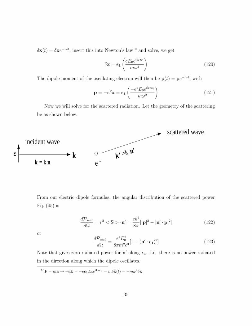
Now we will solve for the scattered radiation. Let the geometry of the scattering

be as shown below.

εincident wave

ke -

scattered wave

k’ =k n’

k = k n

From our electric dipole formulas, the angular distribution of the scattered power

Eq. (45) is

dPscatdΩ

= r2 < S > ·n′ = ck4

8π[|p|2 − |n′ · p|2] (122)

ordPscatdΩ

=e4E2

0

8πm2c3[1− (n′ · ε1)2] (123)

Note that gives zero radiated power for n′ along ε1. I.e. there is no power radiated

in the direction along which the dipole oscillates.

10F = ma→ −eE = −eε1E0eik·x0 = mδx(t) = −mω2δx

35

We may determine the differential cross section for scattering by dividing the

radiated power per solid angle obtained above by the incident power per unit area

(the incident Poynting vector).

Sin =c

8π(E×B∗) =

c

8πE2

0 (124)

thusdσ

dΩ=

1

|Sin|dPscatdΩ

=e4

m2c4

(1− (n′ · ε1)2

)(125)

ordσ

dΩ= r2

0

(1− (n′ · ε1)2

)(126)

where r0 = e2/mc2 = 2.8 × 1013 cm is the classical scattering radius of an electron.

This is the formula for Thomson scattering of incident light polarized along ε1.

5.2 Scattering of Unpolarized Light from an Electron

Now suppose that the incident light is unpolarized. Then the cross section is the

average of the cross sections for the two possible polarizations ε1 and ε2 of the incident

wave (why?).

(dσ

dΩ

)

unpol

=1

2

2∑

i=1

r20

(1− (n′ · εi)2

)(127)

= r20 −

1

2

2∑

i=1

r20

((n′ · εi)2

). (128)

From the fact that (ε1, ε2, and n) form an orthonormal triad of unit vectors, one

may show that (dσ

dΩ

)

unpol

=1

2r2

0

(1 + (n′ · n)2

)(129)

This may be rewritten as

(dσ

dΩ

)

unpol

=1

2r2

0

(1 + cos2(θ)

)(130)

36

where θ is the scattering angle of the unpolarized radiation. From this we can see

that the scattering in predominantly forward (θ = 0), and backscattering (θ = π).

The total cross sections may be obtained by integrating the differential cross

sections. Thus

σpol =8π

3r2

0 (131)

and

σunpol =1

2(σpol(ε1) + σpol(ε2)) = σpol (132)

5.3 Elastic Scattering From a Molecule

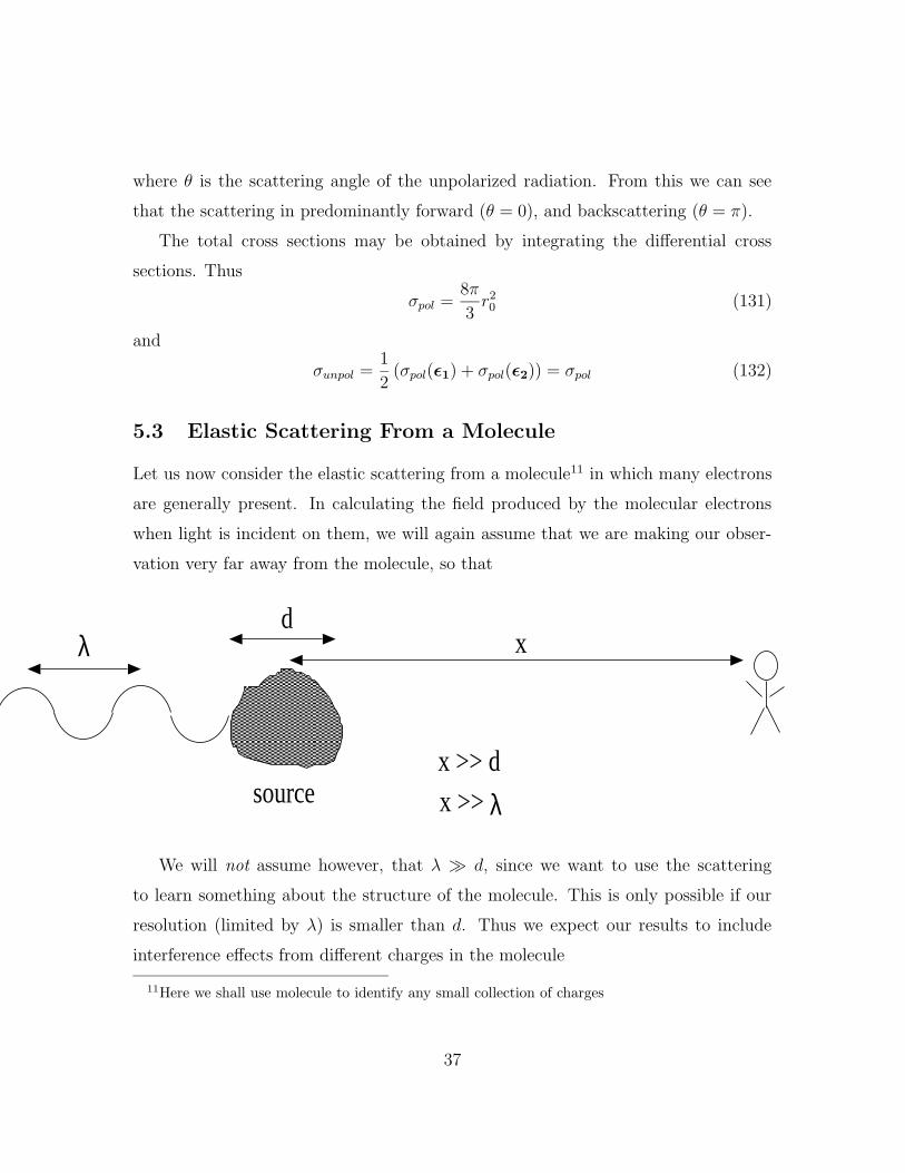
Let us now consider the elastic scattering from a molecule11 in which many electrons

are generally present. In calculating the field produced by the molecular electrons

when light is incident on them, we will again assume that we are making our obser-

vation very far away from the molecule, so that

source

λd

x

x >> dx >> λ

We will not assume however, that λ À d, since we want to use the scattering

to learn something about the structure of the molecule. This is only possible if our

resolution (limited by λ) is smaller than d. Thus we expect our results to include

interference effects from different charges in the molecule

11Here we shall use molecule to identify any small collection of charges

37

Cu

O

O

R

Figure 2: Rays scattered from different elements of the basis, and from different places

on the atom, interfere giving the scattered intensity additional structure described by

the form factor S and the atomic form factor f , respectively.

From page 9, the vector potential produced by the i’th electron in the molecule is

Ai(x) =eikr

cr

∫d3x′ Ji(x

′)e−ik(n·x′). (133)

This expression includes just the current of the i’th electron, and assumes xÀ λ and

xÀ d, as well as a harmonic time dependence. To find the current Ji(x′) for the i’th

electron, we note that the classical current density of an electron is

Ji(x′, t) = −evi(t)δ(x′ − xi) (134)

where (xi,vi) are the location and velocity of the i’th electron. If the electron is

exposed to an incident electromagnetic plane wave, we find that

xi(t) = xi,0 + δxi(t) (135)

δxi(t) = ε1

(eE0

mω2eik·xie−iωt

)(136)

From this we can find the electron velocity, and hence the current

Ji(x′) = ε1

(ie2E0

mωeik·xiδ(x′ − xi)

). (137)

38

In this we have taken out the harmonic time term. Thus the vector potential of the

scattered field generated by the i’th electron in the molecule is

Ai(x) = ε1ie2E0

mω

eikr

crei(k−k′)·xi (138)

where k′ = kn′ is the scattered wave vector and k = kn is the incident wave vector.

We define the vector q = k − k′ which is (1/h times) the momentum transfer from

the photon to the electron, then the total vector potential of the scattered field is

A(x) =∑

i

Ai(x) = ε1ie2E0

mω

eikr

cr

∑

i

eiq·xi (139)

This differs from the vector potential due to a single scattering electron only

through the factor∑i eiq·xi . Since this factor is independent of the observation point

x, the resulting B and E fields are likewise those of a single scattering multiplied

by a factor of∑i eiq·xi . Thus we may immediately write down the differential cross

sections. For polarized light

(dσ

dΩ

)

pol

=[r2

0

(1− (n′ · ε1)2

)]∣∣∣∣∣∑

i

eiq·xi∣∣∣∣∣

2 (140)

where the first term in brackets is the single-electron result, and the second term is

the structure factor. For unpolarized light

(dσ

dΩ

)

unpol

=[1

2r2

0

(1 + (n′ · n)2

)]∣∣∣∣∣∑

i

eiq·xi∣∣∣∣∣

2 (141)

We see that from a measurement of the differential cross section, we may learn

about the structure of the object from which we are scattering light. Let’s examine

the structure factor in more detail.

∑

i

eiq·xi =∫

Vd3x

∑

i

eiq·xiδ(x− xi) (142)

=∫

Vd3x eiq·x

∑

i

δ(x− xi) (143)

39

However,∑

i

δ(x− xi) = nel(x) (144)

which is the electron number density at position x, thus

∑

i

eiq·xi =∫

Vd3x eiq·xnel(x) = nel(−q) (145)

where nel(−q) is the Fourier transform of the electron density. Thus, our differential

cross sections are, for polarized light:(dσ

dΩ

)

pol

=[r2

0

(1− (n′ · ε1)2

)] [|nel(−q)|2

], (146)

and for unpolarized light(dσ

dΩ

)

unpol

=[1

2r2

0

(1 + (n′ · n)2

)] [|nel(−q)|2

](147)

Since q = k − k′ depends upon the scattering angle and the wave number of the

incident photon, a scan over θ and/or k gives you information about the electron

density on the target.

5.3.1 Example: Scattering Off a Hard Sphere

Single sphericalmolecule witha sharp cutoffin its electrondistribution

R

z electrons

40

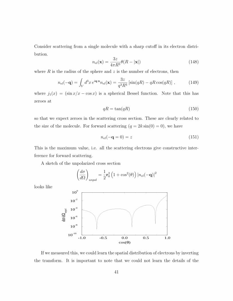
Consider scattering from a single molecule with a sharp cutoff in its electron distri-

bution.

nel(x) =3z

4πR3θ(R− |x|) (148)

where R is the radius of the sphere and z is the number of electrons, then

nel(−q) =∫

Vd3x eiq·xnel(x) =

3z

q3R3[sin(qR)− qR cos(qR)] , (149)

where j1(x) = (sin x/x− cos x) is a spherical Bessel function. Note that this has

zeroes at

qR = tan(qR) (150)

so that we expect zeroes in the scattering cross section. These are clearly related to

the size of the molecule. For forward scattering (q = 2k sin(0) = 0), we have

nel(−q = 0) = z (151)

This is the maximum value, i.e. all the scattering electrons give constructive inter-

ference for forward scattering.

A sketch of the unpolarized cross section(dσ

dΩ

)

unpol

=1

2r2

0

(1 + cos2(θ)

)|nel(−q)|2

looks like

-1.0 -0.5 0.0 0.5 1.0cos(θ)

10-10

10-8

10-6

10-4

10-2

100

dσ/dΩ

unpo

l

If we measured this, we could learn the spatial distribution of electrons by inverting

the transform. It is important to note that we could not learn the details of the

41

electron wavefunctions since all the phase information is lost. I.e., the cross section

just measures the modulus squared of nel, and so phase information is lost.

5.3.2 Example: A Collection of Molecules

A collection of molecules,each with an electronicdistribution n ( )

0x

O

R j

In a macroscopic sample, the total electron density is made up of two parts: the elec-

tron distribution within the molecules, and the distribution of the molecules within

the sample. For simplicity, let’s assume that the sample contains just one type of

molecule, each of which has an electron density n0(x). The total electron number

density is then

nel(x) =∑

j

n0(x−Rj) (152)

where Rj is the position of the j’th molecule. The Fourier transform of this is

nel(−q) =∫

Vd3x eiq·xnel(x) =

∑

j

eiq·Rjn0(−q) (153)

42

which is a weighted sum of the Fourier transforms for each molecule. We see that

then the cross section will include the factor

|n0(−q)|2∣∣∣∣∣∣∑

j

eiq·Rj

∣∣∣∣∣∣

2

(154)

From above, we know that n0(−q = 0) = z, the number of electrons in a molecule,

so we may write

n0(−q) = zF (q) (155)

where F (q) is called the form factor of the molecule which is normalized to unity for

q = 0. Thus the unpolarized differential cross section becomes

(dσ

dΩ

)

unpol

=1

2z2r2

0(1 + cos2(θ)) |F (q)|2∣∣∣∣∣∣∑

j

eiq·Rj

∣∣∣∣∣∣

2

(156)

In general, we will not know where all the molecules are, nor do we necessarily care.

Thus we will look at an average of the term which describes the distribution of the

molecules.⟨∣∣∣∣∣∣∑

j

eiq·Rj

∣∣∣∣∣∣

2⟩=∑

jj′

⟨eiq·(Rj−Rj′)

⟩≈ N

∑

j

⟨eiq·(Rj−R0)

⟩≡ NS(q) (157)

where N is the number of molecules in the sample, R0 is the position of the origin,

and S(q) is the structure factor of the sample. The approximation is justified by the

fact that (neglecting finite-size effects) each link between sites occurs about N times.

This link occurrsabout N times.

43

S(q) =∑

j

⟨eiq·(Rj−R0)

⟩= 1 +

∑

j 6=0

⟨eiq·(Rj−R0)

⟩(158)

Note that this goes to 1 as |q| → ∞. Then, using the same procedure detailed before,

this becomes

NS(q) = V∫

Vd3x eiq·x 〈n(x)n(0)〉 (159)

where V is the sample volume, and n(x) is the number density of molecules in the

sample.

Here, 〈n(x)n(0)〉 tell us about correlations between molecular positions.

〈n(x)n(0)〉 = (n(0))2 g(x) (160)

where g(x) is just the probability of finding a molecule at x if there is one at the origin.

This is the normalized two-body correlation function. We see that if the molecular

form factor is known, then a measurement of the differential cross section tells us

about the Fourier transform of g(x). This is the key to using x-ray (or neutron, etc)

scattering to determine the internal structure of materials.

(dσ

dΩ

)

unpol

=1

2z2r2

0(1 + cos2(θ)) |F (q)|2 V (n(0))2 g(q)

Liquid Crystal

g( )x g( )x

r r

1st peak at meanintermolecularspacing

Averages to 1at large r

latticespacing

44

6 Diffraction

In this section we will discuss diffraction which is related to scattering. The proto-

typical setup is shown below in which radiation from a source is diffracted through

an opaque screen with one or more holes in it.

screen

observersource

Clearly, diffraction is the study of the propagation of light or radiation, or rather

the deviation of light from rectilinear propagation. As undergraduates we all learned

that the propagation of light was governed by Huygen’s Principle that every point

on a primary wavefront serves a the source of spherical secondary wavelets such that

the primary wavefront at some later time is the envelope of these wavelets. Moreover,

the wavelets advance with a speed and frequency equal to that of the primary wave at

each point in space.12. This serves as the paradigm for our study of geometric optics.

Diffraction is the first crisis in this paradigm.

To see this consider wave propagation in a ripple tank through an aperture.

12Hecht-Zajac, page 60

45

d

a) b)

λwaveflow

In the figure, wavefronts are propagating toward the aperture from the bottom of

each box. In case a) the wavelength λ is much smaller than the size of the aperture d.

In this case, the diffracted waves interfere destructively except immediately in front

of the aperture. In case b), λÀ d, and no such interference is is observed.

Huygen’s principle cannot explain the difference between cases a) and b), since

it is independent of any wavelength considerations, and thus would predict the same

wavefront in each case. The difficulty was resolved by Fresnel. The corresponding

Huygens-Fresnel principle states that every unobstructed point of a wavefront,at

a given instant of in time, serves as a source of spherical secondary wavelets of the

same frequency as the source. The amplitude of the diffracted wave is the sum of

the wavelets considering their amplitudes and relative phases13. Applying these ideas

clarifies case a). Here what is happening is that the wavelets from the right and

left sides of the aperture interfere constructively in front of the aperture (since they

travel the same distance and hence remain in phase), whereas these wavelets interfere

destructively to the sides of the aperture (since they travel two paths with length

differences of order λ/2). In case b), we approach the limit of a single point source

13Hecht-Zajac, page 330

46

of spherical waves. Beside being rather hypothetical, the Huygens-Fresnel principle

involves some approximations which we will discuss later; however, Kirchoff showed

that the Huygen’s-Fresnel principle is a direct consequence of the wave equation.

6.1 Scalar Diffraction Theory: Kirchoff Approximation

This problem could be solved using the techniques we just developed to treat scatter-

ing. I.e. by considering the dynamics of the charged particles in the screen, and then

calculating the scattered radiation generated by these particles. However, diffraction

is conventionally treated as a boundary value problem in which the presence of the

screen is taken into account with boundary conditions on the wave.

Several excellent references for this problem are worth noting:

1. B.B. Baker and E.T. Copson, The Mathematical Theory of Huygens Prin-

ciple, (Clarendon Press, Oxford, 1950).

2. Landau and Lifshitz, The Classical Theory of Fields.

3. L. Eyges, The Classical Electromagnetic Field, (Addison-Wesley, Reading,

1972).

4. Hecht-Zajac, Optics, (Addison-Wesley, Reading, 1979).

The Baker reference, especially, has a good discussion of the limits of the Kirchoff

approximation, of course, Landau and Lifshitz have an excellent discussion of the

physics, but Hecht-Zajac’s discussion is perhaps the most elementary, and will often

be quoted here.

The typical question we ask is, given a strictly monochromatic point source S,

what resulting radiation is observed at the point O on the opposite side of the screen.

At first this approach may seem to limit us just to point sources. The case of a real

extended source which emits non-monochromatic light does not, however, require

special treatment. This is because of the linearity of our equations and the complete

47

independence (incoherence) of the light emitted by different points of the source. The

interference terms average to zero. Thus the total diffraction pattern is simply the

sum of the intensity distributions obtained from the diffraction of the independent

components of the light.

screen

observermonochromaticpoint source

ei tω

To treat the theory of diffraction, a number of approximations will be necessary.

• First, we assume that we can neglect the vector nature of the electromagnetic

fields, and work instead with a scalar complex function ψ (a component of E

or B, or the single polarization observed in the ripple tank discussed above).

In principle, ψ is any of the three components of either E or B. In practice,

however, the polarization of the radiation is usually ignored and the intensity

of the radiation at a point is usually taken as |ψ(x, t)|2. This first assumption

limits the number of geometries we can treat.

• Second, we will generally assume that λ/d¿ 1, where d is the linear dimension

of the aperture or obstacle.

• The third assumption is that we will only look for the first correction to geo-

metric optics due to diffraction. This is often called the Kirchoff approximation,

which will be discussed a bit later. (This set of approximations are sometimes

also called the Kirchoff approximation scheme.)

48

We then impose the boundary condition14

ψ(x, t) = 0 everywhere on the screen (161)

We will assume that ψ obeys the wave equation, and the source is harmonic so that

it emits radiation of frequency ω, hence

ψ(x, t) = ψ(x)e−iωt . (162)

Thus the spatial wave function obeys the Helmholtz equation

22ψ = (∇2 + k2)ψ(x) = 0 ,with k = ω/c (163)

if we assume that the waves propagate in a homogeneous medium and restrict our

observations to points away from the source S. As always, the physical quantities

will be the real amplitude < (ψ(x)e−iωt), and the modulus squared which denotes the

time-averaged intensity.

Let’s consider just the observation points in the volume V below which is bounded

by the screen (z = 0 plane), and a hemisphere at infinity.

S

z=0

surface S which includesthe plane at z=0.

VolumeV

(z > 0)(z < 0)

14Note that we only impose one boundary condition on the screen. This is to avoid the difficulties

when both boundary conditions (Neumann and Dirichlet) are imposed, as discussed in Jackson on

page 429

49

Then, everywhere within V , the Helmholtz equation 22ψ = 0 is obeyed since the

source lies outside of V . To find ψ within V , we use Green’s theorem

∫

Vd3x′

(ψ(x′)∇′2φ(x′)− φ(x′)∇′2ψ(x′)

)=∫

Sd2x′ n′·(ψ(x′)∇′φ(x′)− φ(x′)∇′ψ(x′)) ,

(164)

or, adding and subtracting k2ψ(x′)φ(x′) from the first integrand, we get

∫

Vd3x′

(ψ(x′)(∇′2 + k2)φ(x′)− φ(x′)(∇′2 + k2)ψ(x′)

)=∫

Sd2x′ n′·(ψ(x′)∇′φ(x′)− φ(x′)∇′ψ(x′))

(165)

This works for any two functions ψ and φ. We will take ψ(x′) to be the wave ampli-

tude, and take φ(x′) = G(x,x′), where the Dirichlet Green’s function satisfies

(∇2 + k2)G(x,x′) = −4πδ(x− x′) in V (166)

i.e., it is the response to a unit point source so that in free space G(x,x′) = eik|x−x′||x−x′| .

However, need to solve for G with boundary conditions

G(x,x′) = 0 for x′ on S . (167)

since we will be using Dirichlet boundary conditions on ψ: We will specify the value

of ψ(x) (as opposed to its derivative) on the boundary S. Now using the facts that

(∇2 + k2)G(x,x′) = −4πδ(x− x′) in V (168)

(∇2 + k2)ψ(x) = 0 in V (169)

and that

G(x,x′) = 0 for x′ on S (170)

this Green’s theorem becomes (the Kirchoff Integral)

ψ(x) = − 1

4π

∫

Sd2x′ n′ · (ψ(x′)∇′G(x,x′)) (171)

To proceed further we must determine the form of G(x,x′) and we must now

specify ψ(x′) on the surface S. For an infinite planar screen the Green’s function is

50

given by the method of images (analogously to the electrostatic case)

G(x,x′) =eik|x−x′|

|x− x′| −eik|x−y′|

|x− y′| (172)

x’y’

image

where x′ = (x′, y′, z′) is in V , but y′ = (x′, y′,−z′) (the image point) is not. This

satisfies (∇2 +k2)G(x,x′) = −4πδ(x−x′) in V , and vanishes both on the plane z ′ = 0

and on the hemisphere at infinity. Note that it vanishes as 1/r′2 as r′ → ∞. From

this it is clear that the integral

ψ(x) = − 1

4π

∫

Sd2x′ n′ · (ψ(x′)∇′G(x,x′)) (173)

has a vanishing contribution from the hemisphere at infinity, since ψ(x′) vanishes at

least as fast as 1/r′ as r′ →∞ (since it is a solution of the wave equation for a finite

source). Furthermore, from the boundary condition

ψ(x′) = 0 on the screen (174)

we can see that the integral only gets a nonzero contribution from the opening

ψ(x) = − 1

4π

∫

openingd2x′ n′ · (ψ(x′)∇′G(x,x′)) . (175)

So far we have made an exact evaluation of our scalar theory. However, to proceed

we must make an approximation. We will assume that the value of ψ(x′) in the

opening will be the same as if the screen was not there at all. This means that the

wavelength we are considering must be small compared to to characteristic size of

the problem (i.e. the size of the opening). As a result, our formalism will yield just

the the lowest-order correction due to diffraction to the results of geometrical or ray

optics. This approximation is called the Kirchoff approximation.

51

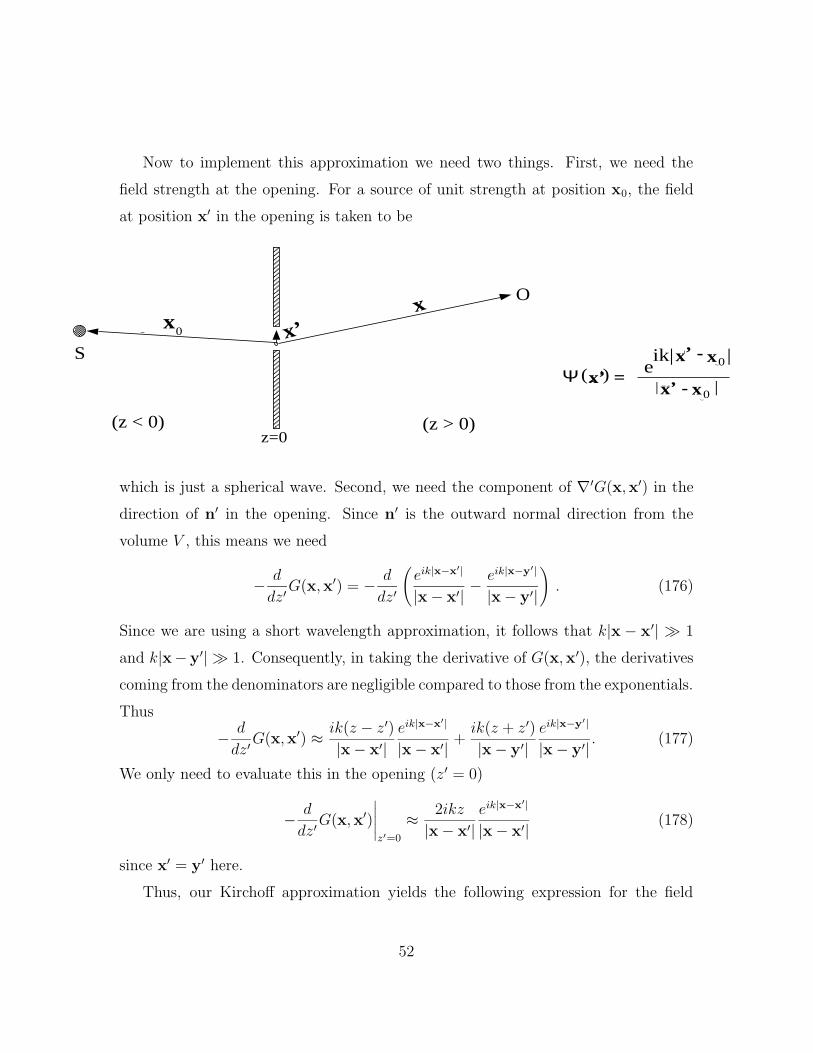
Now to implement this approximation we need two things. First, we need the

field strength at the opening. For a source of unit strength at position x0, the field

at position x′ in the opening is taken to be

S

z=0(z > 0)(z < 0)

Or

r’r0

Ψ ( )r’ =r’ - r0| |

eik| |r’ - r0

x0

xx’

x

xx’

x0

x0 |

which is just a spherical wave. Second, we need the component of ∇′G(x,x′) in the

direction of n′ in the opening. Since n′ is the outward normal direction from the

volume V , this means we need

− d

dz′G(x,x′) = − d

dz′

(eik|x−x′|

|x− x′| −eik|x−y′|

|x− y′|

). (176)

Since we are using a short wavelength approximation, it follows that k|x − x′| À 1

and k|x− y′| À 1. Consequently, in taking the derivative of G(x,x′), the derivatives

coming from the denominators are negligible compared to those from the exponentials.

Thus

− d

dz′G(x,x′) ≈ ik(z − z′)

|x− x′|eik|x−x′|

|x− x′| +ik(z + z′)

|x− y′|eik|x−y′|

|x− y′| . (177)

We only need to evaluate this in the opening (z ′ = 0)

− d

dz′G(x,x′)

∣∣∣∣∣z′=0

≈ 2ikz

|x− x′|eik|x−x′|

|x− x′| (178)

since x′ = y′ here.

Thus, our Kirchoff approximation yields the following expression for the field

52

observed at x

ψ(x) = − 1

4π

∫

openingd2x′ n′ · (ψ(x′)∇G(x,x′)) (179)

= − 1

4π

∫

openingd2x′

2ikz

|x− x′|eik|x−x′|

|x− x′|eik|x0−x′|

|x0 − x′| . (180)

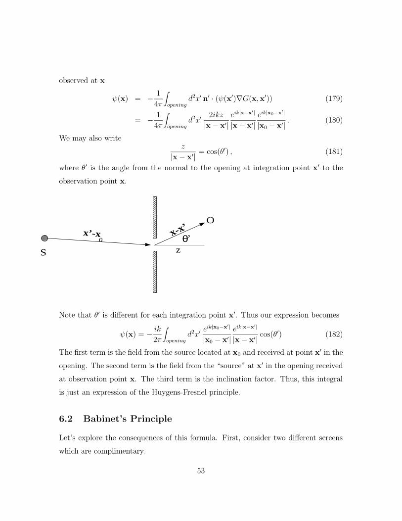
We may also writez

|x− x′| = cos(θ′) , (181)

where θ′ is the angle from the normal to the opening at integration point x′ to the

observation point x.

S z0

x’-x

O

θ’x-x’

Note that θ′ is different for each integration point x′. Thus our expression becomes

ψ(x) = − ik2π

∫

openingd2x′

eik|x0−x′|

|x0 − x′|eik|x−x′|

|x− x′| cos(θ′) (182)

The first term is the field from the source located at x0 and received at point x′ in the

opening. The second term is the field from the “source” at x′ in the opening received

at observation point x. The third term is the inclination factor. Thus, this integral

is just an expression of the Huygens-Fresnel principle.

6.2 Babinet’s Principle

Let’s explore the consequences of this formula. First, consider two different screens

which are complimentary.

53

σσ

One has an opening, labeled σ, while the other is just a disk. For the second screen

the ”opening” is the entire plane z = 0 except for the disk. This opening is the

compliment of σ, so we will call it σ.

We notice something interesting about the amplitudes received at the point O in

the two complimentary cases, we have

ψ(x) = − 1

4π

∫

σd2x′ n′ · (ψ(x′)∇G(x,x′)) (183)

ψ(x) = − 1

4π

∫

σd2x′ n′ · (ψ(x′)∇G(x,x′)) (184)

The sum of these two amplitudes is then

ψ(x) + ψ(x) = − 1

4π

∫

σ+σd2x′ n′ · (ψ(x′)∇G(x,x′)) (185)

However, σ + σ represents the entire plane z = 0. Thus ψ(x) + ψ(x) represents the

amplitude detected at x if there was no screen at all. In other words ψ(x) + ψ(x)

includes no diffraction.

To interpret this, note that ψ(x) may be written as

ψ(x) = feik|x−x0|

|x− x0|+ ψdiff (x) (186)

where f is a ray optic amplitude. If f = 0, then there is no line-of-sight from the

observer to the source, while if f = 1, then there is. The second term is the amplitude

due to diffraction of the wave. Returning to our amplitudes ψ(x) and ψ(x), we see

54

that one will have f = 0 and the other f = 1, so that the sum will include a term

eik|x−x0|/|x− x0|. In fact, this is all it will include, since ψ+ψ includes no diffraction.

Thus, we see that the diffraction amplitudes for complimentary screens cancel. This is

Babinet’s Principle. It says that solving one diffraction problem is tantamount to

solving its compliment. However, Babinet’s principle does not say that the intensities

will cancel in the two cases! We will see some consequences of Babinet’s principle in

what follows

6.3 Fresnel and Fraunhofer Limits

Lets return to our expression for ψ(x) in the Kirchoff approximation. Since we assume

that the wavelength is small, it follows that

kaÀ 1 kr0 À 1 kr À 1 (187)

where a is the typical aperture size, r0 is the distance from the screen to the source,

and r is the distance to the observer.

In general these approximations should be applied to the expression for ψ(x) only

after the integral over the opening has been carried out. This can be done for some

simple geometries (as in the homework). What we will do here is to insert the above

limits into the Kirchoff approximate expressions for ψ(x). In what follows, we will

restrict our attention to apertures, not discs. By doing this it follows that r ′ will

have an upper limit a, so kr′ À 1. In practice, the restriction to apertures is not

a real limitation since Babinet’s principle allows us to calculate the the diffraction

amplitude for a disk from the diffraction amplitude for the complimentary screen.

Once again, our expression for ψ(x) is

ψ(x) = − ik2π

∫

openingd2x′

eik|x0−x′|

|x0 − x′|eik|x−x′|

|x− x′| cos(θ′) . (188)

Now if a/r0 and/or a/r are not small, then we are limited in what further approx-

imations are possible since r′ is not necessarily small compared to either r or r0.

55

This limit is called Fresnel Diffraction, in which the source and/or the observation

points are close enough to the aperture that we must worry about the diffraction of

spherical waves. This presents a difficult problem, which we will not treat (but please

see the homework and Landau and Lifshitz, Classical Theory of Fields, Sec. 60).

In the opposite limit, which we will treat, is called Fraunhofer Diffraction. In

this limit

ka > 1 kr0 À 1 kr À 1 a¿ r0 and a¿ r (189)

Note that we specify ka > 1 rather than ka À 1 since we want to solve for the first

finite corrections to the latter inequality, so that

ka2

r0

= ka(a

r0

)¿ 1 and

ka2

r′¿ 1 (190)

Thus we are looking at plane waves instead of spherical waves in this limit.

It is possible to simplify our expression for ψ(x) even further in this limit. Then

|x′ − x0| ≈ r0 −x0 · x′r0

= r0 + n0 · x′ (191)

where n0 is a unit vector from the source to the origin (taken to be the center of the

aperture), so that x0 = −n0r0. Similarly,

|x− x′| ≈ r − n · x′ (192)

where n is a unit vector from the origin to the observer so that x = nr.

SOn

n0

56

Thus,eik|x

′−x0|

|x′ − x0|eik|x−x′|

|x− x′| ≈eik(r+r0)

rr0

eik(n0−n)·x′ (193)

where we have dropped second-order terms coming from the denominators. Further-

more, since r is large compared to the aperture size, it is appropriate to take

cos(θ′) =z

|x− x′| ≈ 1 (194)

inside the integral. Thus in the Fraunhofer limit

ψ(x) = − ik2π

eik(r+r0)

rr0

∫

openingd2x′ eik(n0−n)·x′ (195)

But the incident wave vector was kn, so

k(n0 − n) = kin − kdiff ≡ q (196)

so we finally have

ψ(x) = − ik2π

eik(r+r0)

rr0

∫

openingd2x′ eiq·x

′(197)

7 Example Problems

Let’s consider some examples.

7.1 Example: Diffraction from a Rectangular Aperture

Here the opening is given by |x′| < a and |y′| < b, so the integral above is

∫

openingd2x′ eiq·x

′=∫ a

−adx′ eiqxx

′∫ b

−bdy′ eiqyy

′= 2

sin(qxa)

qx2

sin(qyb)

qy(198)

The amplitude at x is

ψ(x) = −2ikab

π

eik(r+r0)

rr0

(sin(qxa)

aqx

)(sin(qyb)

bqy

)(199)

57

thus, the intensity of the diffracted wave is

I(x) = |ψ(x)|2 = I0

(sin(qxa)

aqx

)2 (sin(qyb)

bqy

)2

(200)

with

I0 =4k2a2b2

π2r20r

2(201)

We see that all of the angular dependence of in this is embodied in the dependence

on q, the momentum transfer. Since we a looking at small-angle scattering, we are

taking q to lie essentially in the x-y plane.

k ink diff q

We see that the nodes of I(x) occur for

qx =mπ

a, m 6= 0, and/or qy =

nπ

b, n 6= 0 (202)

The global maximum (I(x) = I0) occurs for qx = qy = 0, i.e. for forward scattering.

Thus the intensity of the diffracted light looks something like

centralmaximum

lines of nodes

58

We can recover the formula for single-slit diffraction by taking bÀ a, so that our

rectangular aperture becomes a slit of width 2a. Then

θdiffθθ in

θθ in2a sin( ) θdiff2a sin( )

y

x

qx = (kx)in − (kx)diff = k sin(θin)− k sin(θdiff ) (203)

and the condition that there is a node is

qx = k (sin(θin)− sin(θdiff )) =mπ

am 6= 0 . (204)

Since k = 2π/λ, this may be written

2a (sin(θin)− sin(θdiff )) = mλ m 6= 0 (205)

which is the usual expression for a node in single-slit diffraction.

7.2 Example: Diffraction from a Circular Aperture

Here the opening is given by r′ < a. Our Fraunhofer expression for the amplitude at

x is then

ψ(x) = − ik2π

eik(r+r0)

rr0

∫ a

0dr′ r′

∫ 2π

0dφ′eiqr

′ cos(φ′) (206)

59

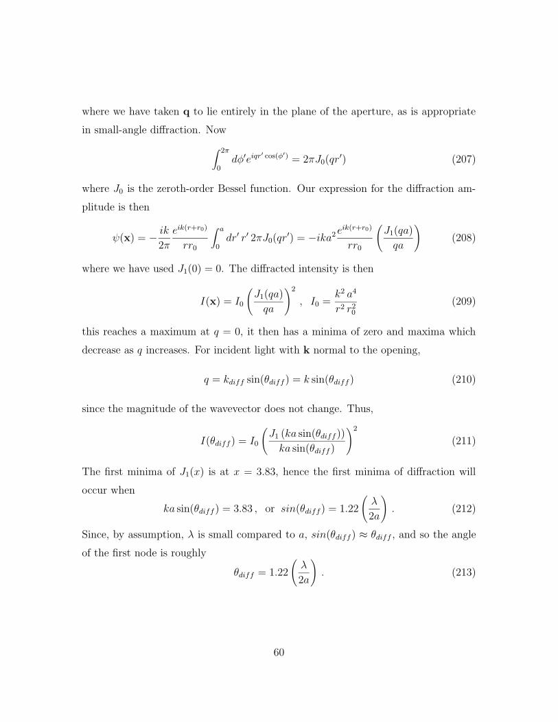
where we have taken q to lie entirely in the plane of the aperture, as is appropriate

in small-angle diffraction. Now

∫ 2π

0dφ′eiqr

′ cos(φ′) = 2πJ0(qr′) (207)

where J0 is the zeroth-order Bessel function. Our expression for the diffraction am-

plitude is then

ψ(x) = − ik2π

eik(r+r0)

rr0

∫ a

0dr′ r′ 2πJ0(qr′) = −ika2 e

ik(r+r0)

rr0

(J1(qa)

qa

)(208)

where we have used J1(0) = 0. The diffracted intensity is then

I(x) = I0

(J1(qa)

qa

)2

, I0 =k2 a4

r2 r20

(209)

this reaches a maximum at q = 0, it then has a minima of zero and maxima which

decrease as q increases. For incident light with k normal to the opening,

q = kdiff sin(θdiff ) = k sin(θdiff ) (210)

since the magnitude of the wavevector does not change. Thus,

I(θdiff ) = I0

(J1 (ka sin(θdiff ))

ka sin(θdiff )

)2

(211)

The first minima of J1(x) is at x = 3.83, hence the first minima of diffraction will

occur when

ka sin(θdiff ) = 3.83 , or sin(θdiff ) = 1.22

(λ

2a

). (212)

Since, by assumption, λ is small compared to a, sin(θdiff ) ≈ θdiff , and so the angle

of the first node is roughly

θdiff = 1.22

(λ

2a

). (213)

60

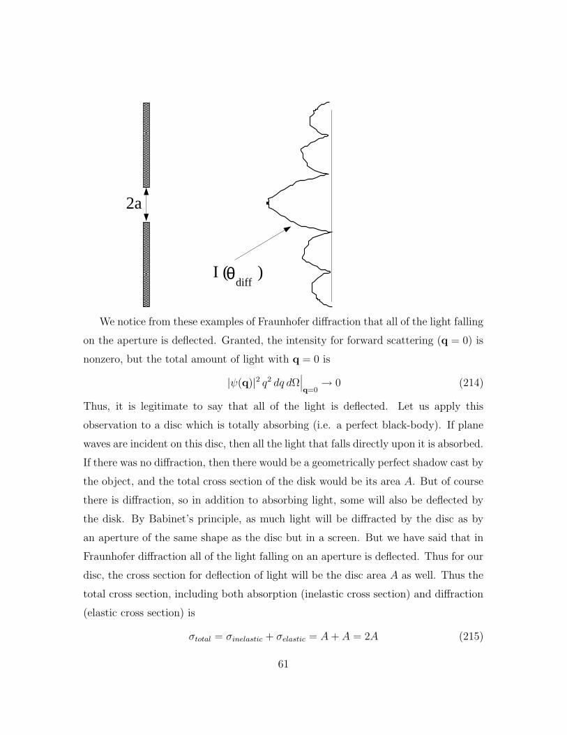
2a

θdiff

I ( )

We notice from these examples of Fraunhofer diffraction that all of the light falling

on the aperture is deflected. Granted, the intensity for forward scattering (q = 0) is

nonzero, but the total amount of light with q = 0 is

|ψ(q)|2 q2 dq dΩ∣∣∣q=0→ 0 (214)

Thus, it is legitimate to say that all of the light is deflected. Let us apply this

observation to a disc which is totally absorbing (i.e. a perfect black-body). If plane

waves are incident on this disc, then all the light that falls directly upon it is absorbed.

If there was no diffraction, then there would be a geometrically perfect shadow cast by

the object, and the total cross section of the disk would be its area A. But of course

there is diffraction, so in addition to absorbing light, some will also be deflected by

the disk. By Babinet’s principle, as much light will be diffracted by the disc as by

an aperture of the same shape as the disc but in a screen. But we have said that in

Fraunhofer diffraction all of the light falling on an aperture is deflected. Thus for our

disc, the cross section for deflection of light will be the disc area A as well. Thus the

total cross section, including both absorption (inelastic cross section) and diffraction

(elastic cross section) is

σtotal = σinelastic + σelastic = A+ A = 2A (215)

61

This is twice the area of the disc. Recall that in this argument we assume that kaÀ 1,

where a is the characteristic size of the disc. In this limit in quantum mechanics one

finds that the cross section for scattering from a sphere of radius a is 2πa2. The factor

of two has the same origins here as it does in quantum mechanics.

7.3 Diffraction from a Cross

1. Given a normally incident wave of frequency ω calculate the diffraction pattern

produced by an opaque screen with an aperture in the shape symmetric cross

of inner dimension a and outer dimension b in the Fraunhofer limit of the scalar

Kirchoff approximation. Very roughly tell what the diffraction pattern will look

like.

2. The correct answer to the first part of this problem also yields the solution to

the diffraction pattern involving a quite different set of apertures. What is this

other set of apertures?

ab

Solution. In the Fraunhoffer limit, we can use Eq. (197) of the notes.

ψ(x) = − ik2π

eik(r+r0)

rr0

∫

openingd2x′ eiq·x

′

where r0 is the distance from the aperture to the source, r is the distance from the

aperture to the observer, and q is the difference between the incident and scattered

62

wavevector. We will take q to lie entirely in the plane of the aperture, as is appropriate

in the small angle limit.

For the geometry in the figure, the integrals may be performed trivially

ψ(x) = − ik2π

eik(r+r0)

rr0

(∫ a

−adx′

∫ a

−ady′ +

∫ a

−adx′

(∫ −a

−bdy′ +

∫ b

ady′)

+∫ a

−ady′

(∫ −a

−bdx′ +

∫ b

adx′))

eiqxx′eiqyy

′

so that

ψ(x) =2ik

πqxqy

eik(r+r0)

rr0

[sin(aqx) sin(bqy) + sin(aqy) sin(bqx)− sin(aqx) sin(aqy)]

The corresponding intensity |ψ(x)|2 will have a central maximum with I ∝ (2ab−a2)2,

and the whole pattern will be symmetric to rotations modulo π/2. By Babinet’s

principle we know that the diffraction from a cross-shaped screen has an amplitude,

that when added to ψ(x), is the same as if there was no diffraction at all.

7.4 Radiation from a Reciprocating Disk

A disc of radius a lies in the z = 0 plane and is centered at the origin. It is uniformly

charged with surface charge density σ, and it rotates around the z-axis with an

angular velocity Ω cos(ωt) where Ω and ω are constants. Assuming that the motion

is nonrelativistic, find the fields in the radiation zone, the angular distribution of

radiated power, and the total radiated power.

Solution. Here we will employ the methods developed to treat the radiation of

harmonic current sources. The current of the rotation disc is (in cylindrical coordi-

nates)

J(x, t) = δ(z)σΩ cos(ωt)ρφ

or, in complex notation

J(x, t) = δ(z)σΩe−iωtρφ = J(x)e−iωt

Then,

f(θ, φ) =1

c

∫

Vd3x′ J(x′)e−ikn·x

′=σΩ

c

∫ a

0ρ′dρ′

∫ 2π

0dφ′ρ′φ′e−ikn·x

′

63

We can use the azimuthal symmetry of the problem, and assume that n is in the xz

plane. Then n = cos θz + sin θx, x′ = ρ′ (cos(φ′)x + sin(φ′)y), and φ′ = cos(φ′)y −sin(φ′)x. For non-relativistic motion Ωa/c ¿ 1, this allows us to keep only the first

nonvanishing term in the exponential, then

f(θ, φ) = −iπka4σΩ

4csin θφ

Hence, in the radiation zone,

B = ikeikr

r(n× f) = −πk

2a4σΩ

4csin θ

eikr

rθ

and

E = B× n =πk2a4σΩ

4csin θ

eikr

rφ

The power distribution is given by

dP

dΩ=ck2

8π

[|f |2 − |n · f |2

]=ck2

8π

π2k2a8σ2Ω2

16c2sin2(θ)

The total power is obtained by integrating over all solid angles

P =π2k4σ2Ω2a8

48c

64