145

7 AGGREGATE SUPPLY AND AGGREGATE DEMAND**

* * This is Chapter 23 in Economics.

C h a p t e r K e y I d e a s

Production and Prices

A. What forces bring persistent and rapid expansion of real GDP?

B. What leads to inflation?

C. Why do we have business cycles?

D. Research on these issues divides economists into schools of thought.

E. The AS-AD model provides a framework for understanding economic growth, inflation, business cycles, and the different schools of economic thought.

O u t l i n e

I. Aggregate Supply

A. Aggregate Supply Fundamentals

1. The aggregate quantity of goods and services supplied depends on three factors:

a) The quantity of labor (L )

b) The quantity of capital (K )

c) The state of technology (T )

2. The aggregate production function, Y = F(L, K, T ), shows how quantity of real GDP supplied, Y, depends on labor, capital, and technology.

3. At any given time, the quantity of capital and the state of technology are fixed but the quantity of labor can vary.

4. The wage rate that makes the quantity of labor demanded equal to the quantity supplied is the equilibrium wage rate. At that wage rate, the level of employment full employment. At full employment, the unemployment rate is called the natural rate of unemployment.

5. Over the business cycle, employment fluctuates around full employment.

C h a p t e r

1 4 6 C H A P T E R 7

6. To study aggregate supply in different sates of the labor market, we distinguish two time frames:

a) Long-run aggregate supply

b) Short-run aggregate supply

B. Long-Run Aggregate Supply

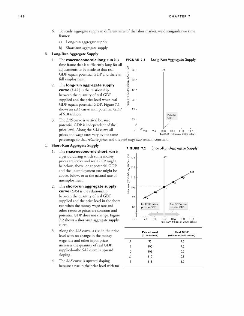
1. The macroeconomic long run is a time frame that is sufficiently long for all adjustments to be made so that real GDP equals potential GDP and there is full employment.

2. The long-run aggregate supply curve (LAS ) is the relationship between the quantity of real GDP supplied and the price level when real GDP equals potential GDP. Figure 7.1 shows an LAS curve with potential GDP of $10 trillion.

3. The LAS curve is vertical because potential GDP is independent of the price level. Along the LAS curve all prices and wage rates vary by the same percentage so that relative prices and the real wage rate remain constant.

C. Short-Run Aggregate Supply

1. The macroeconomic short run is a period during which some money prices are sticky and real GDP might be below, above, or at potential GDP and the unemployment rate might be above, below, or at the natural rate of unemployment.

2. The short-run aggregate supply curve (SAS) is the relationship between the quantity of real GDP supplied and the price level in the short run when the money wage rate and other resource prices are constant and potential GDP does not change. Figure 7.2 shows a short-run aggregate supply curve.

3. Along the SAS curve, a rise in the price level with no change in the money wage rate and other input prices increases the quantity of real GDP supplied—the SAS curve is upward sloping.

4. The SAS curve is upward sloping because a rise in the price level with no

A G G R E G A T E S U P P L Y A N D A G G R E G A T E D E M A N D 1 4 7

change in costs induces firms to increase production; and a fall in the price level with no change in costs induces firms to decrease production.

D. Movements along the LAS and SAS Curves

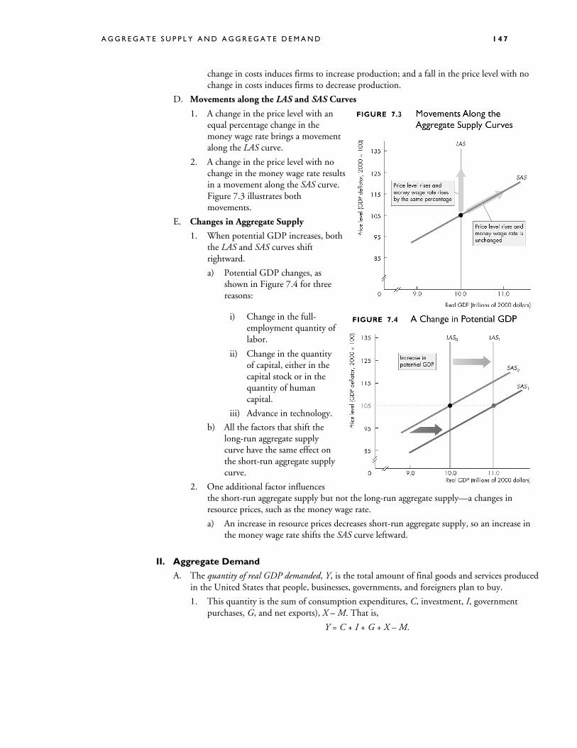
1. A change in the price level with an equal percentage change in the money wage rate brings a movement along the LAS curve.

2. A change in the price level with no change in the money wage rate results in a movement along the SAS curve. Figure 7.3 illustrates both movements.

E. Changes in Aggregate Supply

1. When potential GDP increases, both the LAS and SAS curves shift rightward.

a) Potential GDP changes, as shown in Figure 7.4 for three reasons:

i) Change in the full-employment quantity of labor.

ii) Change in the quantity of capital, either in the capital stock or in the quantity of human capital.

iii) Advance in technology.

b) All the factors that shift the long-run aggregate supply curve have the same effect on the short-run aggregate supply curve.

2. One additional factor influences the short-run aggregate supply but not the long-run aggregate supply—a changes in resource prices, such as the money wage rate.

a) An increase in resource prices decreases short-run aggregate supply, so an increase in the money wage rate shifts the SAS curve leftward.

II. Aggregate Demand

A. The quantity of real GDP demanded, Y, is the total amount of final goods and services produced in the United States that people, businesses, governments, and foreigners plan to buy.

1. This quantity is the sum of consumption expenditures, C, investment, I, government purchases, G, and net exports), X – M. That is,

Y = C + I + G + X – M.

1 4 8 C H A P T E R 7

2. Buying plans depend on many factors and some of the main ones are

a) The price level

b) Expectations

c) Fiscal and monetary policy

d) The world economy

B. The Aggregate Demand Curve

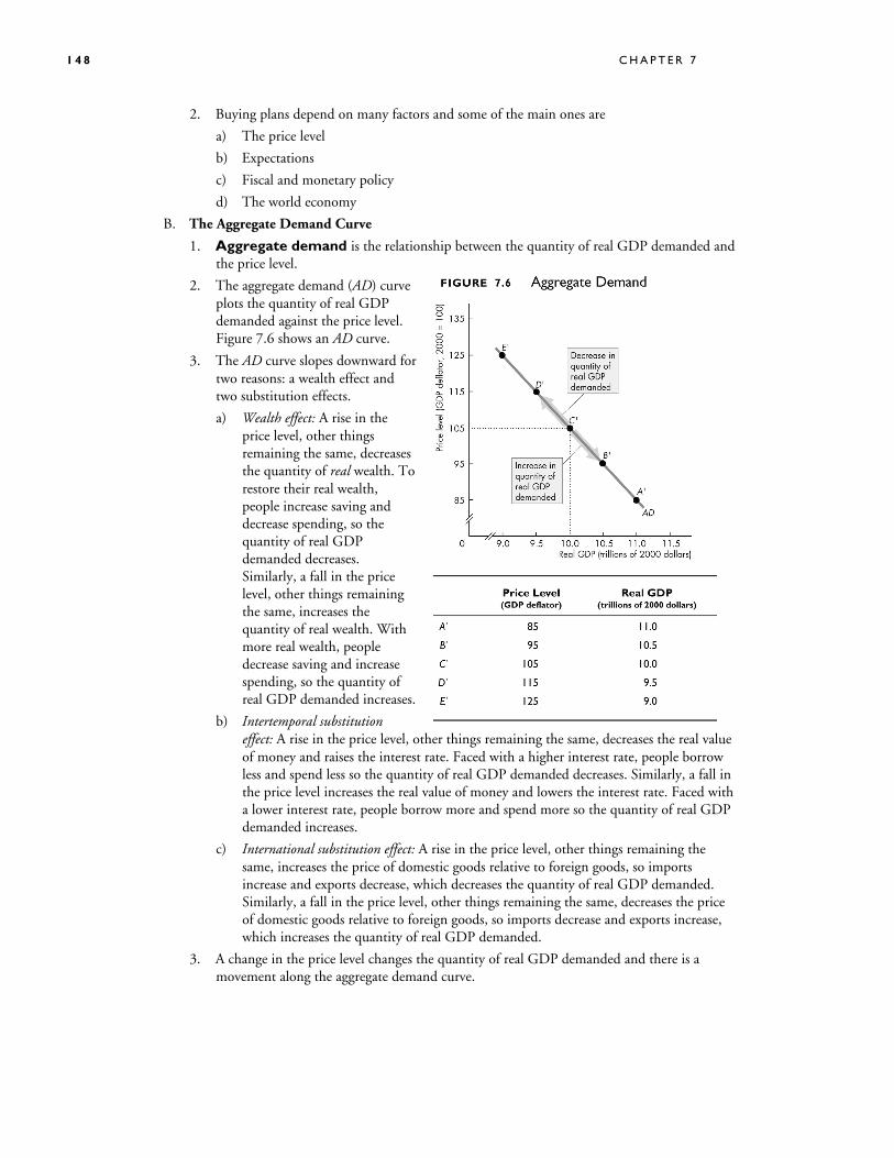
1. Aggregate demand is the relationship between the quantity of real GDP demanded and the price level.

2. The aggregate demand (AD) curve plots the quantity of real GDP demanded against the price level. Figure 7.6 shows an AD curve.

3. The AD curve slopes downward for two reasons: a wealth effect and two substitution effects.

a) Wealth effect: A rise in the price level, other things remaining the same, decreases the quantity of real wealth. To restore their real wealth, people increase saving and decrease spending, so the quantity of real GDP demanded decreases. Similarly, a fall in the price level, other things remaining the same, increases the quantity of real wealth. With more real wealth, people decrease saving and increase spending, so the quantity of real GDP demanded increases.

b) Intertemporal substitution effect: A rise in the price level, other things remaining the same, decreases the real value of money and raises the interest rate. Faced with a higher interest rate, people borrow less and spend less so the quantity of real GDP demanded decreases. Similarly, a fall in the price level increases the real value of money and lowers the interest rate. Faced with a lower interest rate, people borrow more and spend more so the quantity of real GDP demanded increases.

c) International substitution effect: A rise in the price level, other things remaining the same, increases the price of domestic goods relative to foreign goods, so imports increase and exports decrease, which decreases the quantity of real GDP demanded. Similarly, a fall in the price level, other things remaining the same, decreases the price of domestic goods relative to foreign goods, so imports decrease and exports increase, which increases the quantity of real GDP demanded.

3. A change in the price level changes the quantity of real GDP demanded and there is a movement along the aggregate demand curve.

A G G R E G A T E S U P P L Y A N D A G G R E G A T E D E M A N D 1 4 9

C. Changes in Aggregate Demand

1. A change in any influence on buying plans other than the price level changes aggregate demand.

2. The main influences are: expectations, fiscal and monetary policy, and the world economy.

a) Expectations about future income, future inflation, and future profits change aggregate demand.

i) Increases in expected future income increase peoples’ consumption today, and increases aggregate demand.

ii) An increase in the expected inflation rate makes buying goods cheaper today and increases aggregate demand.

iii) An increase in expected future profits boosts firms’ investment, which increases aggregate demand.

b) Fiscal policy is the government’s attempt to influence the economy by setting and changing taxes, making transfer payments, and purchasing goods and services.

i) Disposable income is aggregate income minus taxes plus transfer payments. A tax cut or an increase in transfer payments increases households’ disposable income. An increase in disposable income increases consumption expenditure and increases aggregate demand.

ii) Because government purchases of goods and services are one component of aggregate demand, an increase in government purchases increases aggregate demand.

1 5 0 C H A P T E R 7

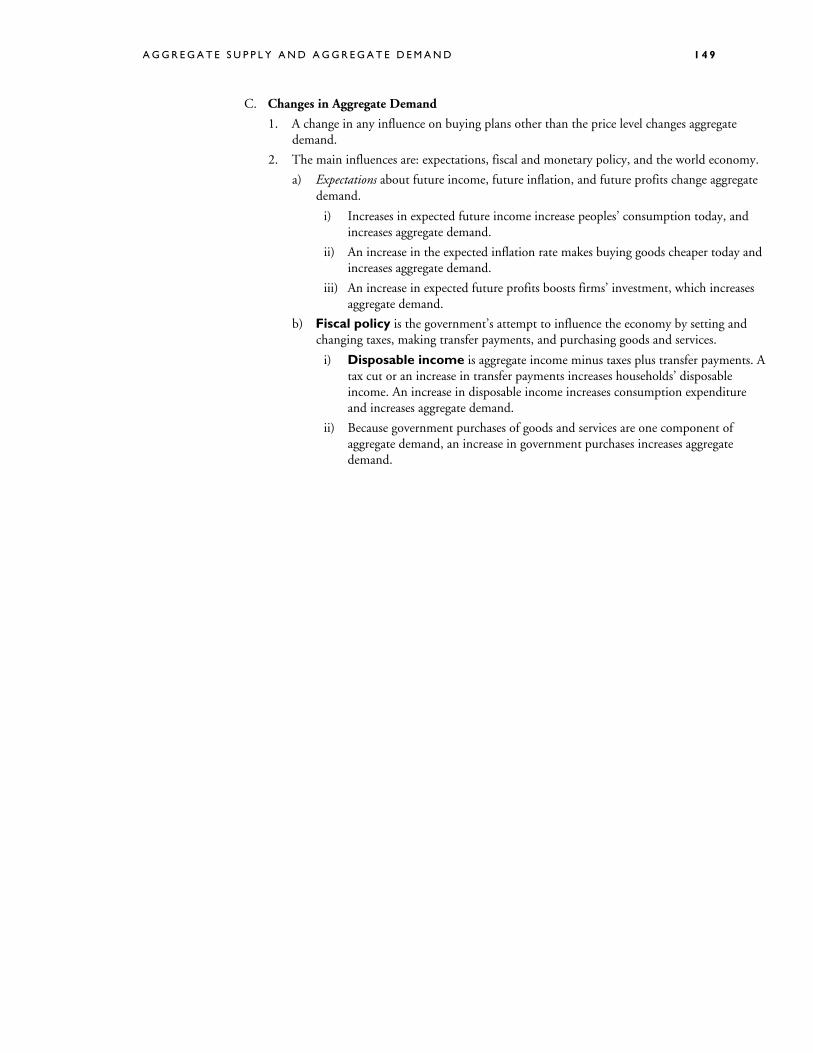
c) Monetary policy is changes in the interest rate and quantity of money in the economy.

i) An increase in the quantity of money increases buying power and increases aggregate demand.

ii) A cut in the interest rate increases expenditure and increases aggregate demand.

d) The world economy influences aggregate demand in two ways:

i) A fall in the foreign exchange rate lowers the price of domestic goods and services relative to foreign goods and services and so increases exports and decreases imports, thereby increasing aggregate demand.

ii) An increase in foreign income increases the demand for U.S. exports and increases aggregate demand.

3. When aggregate demand increases, the AD curve shifts rightward and when aggregate demand decreases, the AD curve shifts leftward. Figure 7.7 illustrates an increase and a decrease in aggregate demand.

III. Macroeconomic Equilibrium

A. Short-Run Macroeconomic Equilibrium

1. Short-run macroeconomic equilibrium occurs when the quantity of real GDP demanded equals the quantity of real GDP supplied. Short-run macroeconomic equilibrium occurs at the point of intersection of the AD curve and the SAS curve.

A G G R E G A T E S U P P L Y A N D A G G R E G A T E D E M A N D 1 5 1

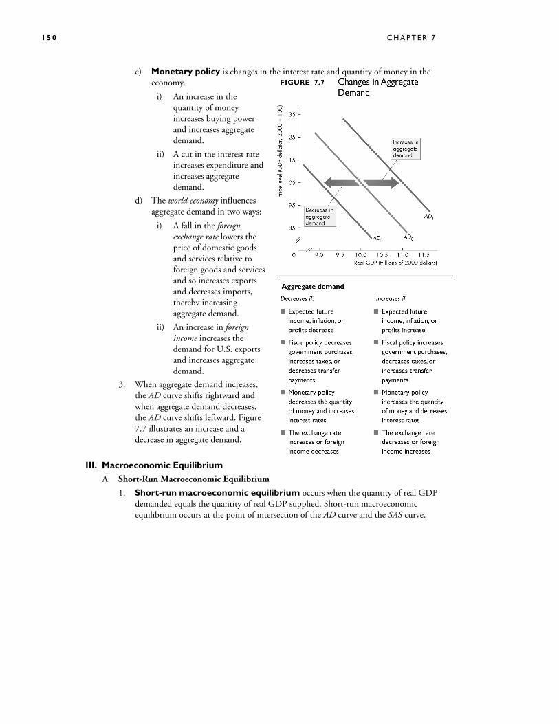
2. Figure 7.8 illustrates a short-run equilibrium.

a) If real GDP is below equilibrium GDP, firms increase production and raise prices; and if real GDP is above equilibrium GDP, firms decrease production and lower prices.

b) These changes bring a movement along the SAS curve toward equilibrium.

3. In short-run equilibrium, real GDP can be greater than or less than potential GDP.

B. Long-Run Macroeconomic Equilibrium

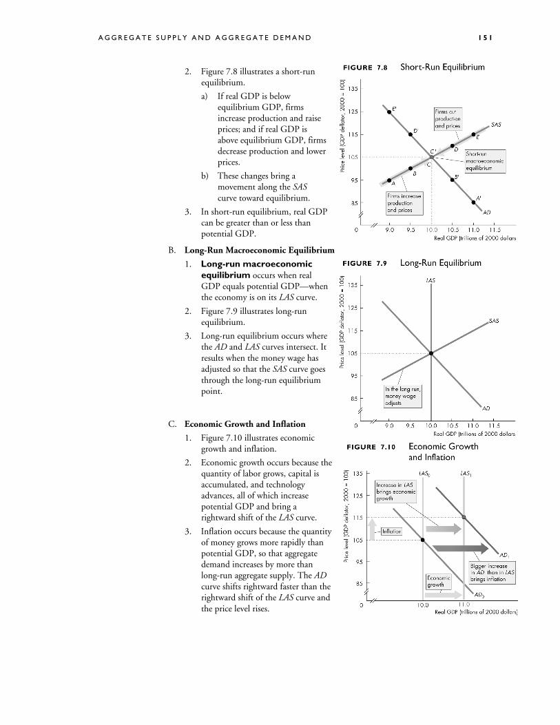
1. Long-run macroeconomic equilibrium occurs when real GDP equals potential GDP—when the economy is on its LAS curve.

2. Figure 7.9 illustrates long-run equilibrium.

3. Long-run equilibrium occurs where the AD and LAS curves intersect. It results when the money wage has adjusted so that the SAS curve goes through the long-run equilibrium point.

C. Economic Growth and Inflation

1. Figure 7.10 illustrates economic growth and inflation.

2. Economic growth occurs because the quantity of labor grows, capital is accumulated, and technology advances, all of which increase potential GDP and bring a rightward shift of the LAS curve.

3. Inflation occurs because the quantity of money grows more rapidly than potential GDP, so that aggregate demand increases by more than long-run aggregate supply. The AD curve shifts rightward faster than the rightward shift of the LAS curve and the price level rises.

1 5 2 C H A P T E R 7

D. The Business Cycle

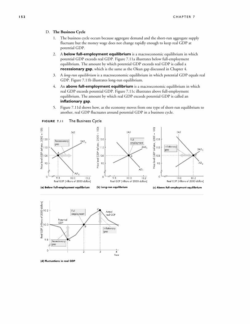
1. The business cycle occurs because aggregate demand and the short-run aggregate supply fluctuate but the money wage does not change rapidly enough to keep real GDP at potential GDP.

2. A below full-employment equilibrium is a macroeconomic equilibrium in which potential GDP exceeds real GDP. Figure 7.11a illustrates below full-employment equilibrium. The amount by which potential GDP exceeds real GDP is called a recessionary gap, which is the same as the Okun gap discussed in Chapter 4.

3. A long-run equilibrium is a macroeconomic equilibrium in which potential GDP equals real GDP. Figure 7.11b illustrates long-run equilibrium.

4. An above full-employment equilibrium is a macroeconomic equilibrium in which real GDP exceeds potential GDP. Figure 7.11c illustrates above full-employment equilibrium. The amount by which real GDP exceeds potential GDP is called an inflationary gap.

5. Figure 7.11d shows how, as the economy moves from one type of short-run equilibrium to another, real GDP fluctuates around potential GDP in a business cycle.

A G G R E G A T E S U P P L Y A N D A G G R E G A T E D E M A N D 1 5 3

E. Fluctuations in Aggregate Demand

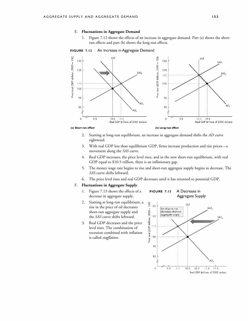
1. Figure 7.12 shows the effects of an increase in aggregate demand. Part (a) shows the short-run effects and part (b) shows the long-run effects.

2. Starting at long-run equilibrium, an increase in aggregate demand shifts the AD curve rightward.

3. With real GDP less than equilibrium GDP, firms increase production and rise prices—a movement along the SAS curve.

4. Real GDP increases, the price level rises, and in the new short-run equilibrium, with real GDP equal to $10.5 trillion, there is an inflationary gap.

5. The money wage rate begins to rise and short-run aggregate supply begins to decrease. The SAS curve shifts leftward.

6. The price level rises and real GDP decreases until it has returned to potential GDP.

F. Fluctuations in Aggregate Supply

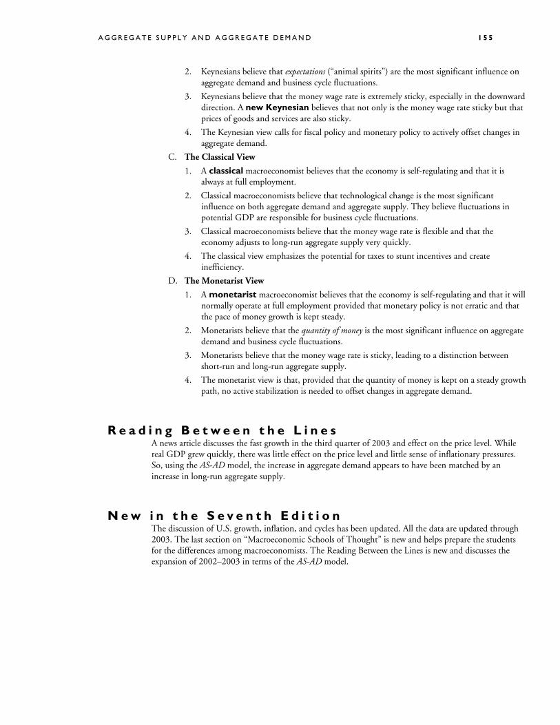
1. Figure 7.13 shows the effects of a decrease in aggregate supply.

2. Starting at long-run equilibrium, a rise in the price of oil decreases short-run aggregate supply and the SAS curve shifts leftward.

3. Real GDP decreases and the price level rises. The combination of recession combined with inflation is called stagflation.

1 5 4 C H A P T E R 7

IV. U.S. Economic Growth, Inflation, and Cycles

A. Figure 7.14 is a scatter diagram of real GDP and the price level each year from 1963 to 2003. The figure also interprets the data in terms of shifting AD, SAS, and LAS curves. The data show economic growth, inflation, and the business cycle between 1963 and 2003.

1. Real GDP and potential GDP grew from $2.8 trillion to $10.3 trillion.

2. The price level rose from 22 to 105.

3. Business cycle expansions alternated with recessions.

B. Economic Growth

Real GDP growth was rapid during the 1960s and 1990s and slower during the 1970s and 1980s.

C. Inflation

Inflation was the most rapid during the 1970s.

D. Business Cycles

Recessions occurred during the mid-1970s, 1982, 1991–1992, and 2001.

V. Macroeconomic Schools of Thought

A. Macroeconomics is an active field of research in which there is much consensus, but also some differing viewpoints, especially about the business cycle.

B. The Keynesian View

1. A Keynesian macroeconomist believes that left alone, the economy would rarely operate at full employment and that to achieve and maintain full employment, active help from fiscal policy and monetary policy is required.

A G G R E G A T E S U P P L Y A N D A G G R E G A T E D E M A N D 1 5 5

2. Keynesians believe that expectations (“animal spirits”) are the most significant influence on aggregate demand and business cycle fluctuations.

3. Keynesians believe that the money wage rate is extremely sticky, especially in the downward direction. A new Keynesian believes that not only is the money wage rate sticky but that prices of goods and services are also sticky.

4. The Keynesian view calls for fiscal policy and monetary policy to actively offset changes in aggregate demand.

C. The Classical View

1. A classical macroeconomist believes that the economy is self-regulating and that it is always at full employment.

2. Classical macroeconomists believe that technological change is the most significant influence on both aggregate demand and aggregate supply. They believe fluctuations in potential GDP are responsible for business cycle fluctuations.

3. Classical macroeconomists believe that the money wage rate is flexible and that the economy adjusts to long-run aggregate supply very quickly.

4. The classical view emphasizes the potential for taxes to stunt incentives and create inefficiency.

D. The Monetarist View

1. A monetarist macroeconomist believes that the economy is self-regulating and that it will normally operate at full employment provided that monetary policy is not erratic and that the pace of money growth is kept steady.

2. Monetarists believe that the quantity of money is the most significant influence on aggregate demand and business cycle fluctuations.

3. Monetarists believe that the money wage rate is sticky, leading to a distinction between short-run and long-run aggregate supply.

4. The monetarist view is that, provided that the quantity of money is kept on a steady growth path, no active stabilization is needed to offset changes in aggregate demand.

R e a d i n g B e t w e e n t h e L i n e s A news article discusses the fast growth in the third quarter of 2003 and effect on the price level. While real GDP grew quickly, there was little effect on the price level and little sense of inflationary pressures. So, using the AS-AD model, the increase in aggregate demand appears to have been matched by an increase in long-run aggregate supply.

N e w i n t h e S e v e n t h E d i t i o n The discussion of U.S. growth, inflation, and cycles has been updated. All the data are updated through 2003. The last section on “Macroeconomic Schools of Thought” is new and helps prepare the students for the differences among macroeconomists. The Reading Between the Lines is new and discusses the expansion of 2002–2003 in terms of the AS-AD model.

1 5 6 C H A P T E R 7

Te a c h i n g S u g g e s t i o n s 1. Economists as a group are ambivalent about the aggregate supply-aggregate demand (AS-AD) model.

Real business cycle theorists, who like to build their models from the base of production functions and preferences, don’t use the model because the AS and AD curves are not independent. Technological change shifts both the AS and AD curves simultaneously and in complicated ways. New Keynesian economists have dropped the model in favor of a dynamic variant that places the inflation rate on the y-axis and the output gap (real GDP minus potential GDP as a percentage of potential GDP) on the x-axis.

Despite attacks on the model from both sides of the doctrinal spectrum, those of us who spend a good part of our professional lives teaching the principles course recognize the AS-AD model as the key macroeconomic model. For us, the model plays a similar role in the organization of the macroeconomics to that played by the demand and supply model in microeconomics. That is the view taken in this textbook.

The AS-AD model is the best model currently available for introducing students to macroeconomics. It enables them to gain insights into the way the economy works, to organize their study of the subject, and to understand the debates surrounding the effects of policies designed to improve macroeconomic performance.

Devoting about a week of lecture time to the AS-AD model is worthwhile. At this point the students don’t yet have the background to appreciate all the details that go into the aggregate demand and aggregate supply curves. But they are able to grasp the basic purpose of the model. Your goal at this point in the course is to help them understand the components of the model intuitively and to put the model to work using some of its more simple and obvious features. (The situation is very similar to that at the beginning of the microeconomics sequence when you teach demand and supply At that stage, the students don’t know about the consumer problem that lies behind the demand curve and the model of perfect competition that lies behind the supply curve when they study demand and supply at the beginning of their microeconomics course. But they can appreciate the intuition on the demand and supply curves and use the model to generate predictions.)

2. Aggregate Supply The flavor of the Classical-Keynesian controversy. If you want to convey the flavor of one of the biggest

controversies in macroeconomics, you can do so at this early stage of the course by using only the aggregate supply curves. The difference between the upward-sloping SAS and the vertical LAS lies at the core of the disagreement between Classical economists who believe that wages and prices are highly flexible and adjust rapidly and Keynesian economists who believe that the money wage rate in particular adjusts very slowly.

Along the LAS curve—two things happening. Students seem comfortable with the idea that the SAS curve has a positive slope; but they seem less at ease with the vertical LAS curve. Emphasize (as the textbook does) the crucial idea that along the LAS curve two sets of prices are changing — the prices of output and the prices of resources, especially the money wage rate. Once they get this point, students quickly catch on to the result that firms won’t be motivated to change their production levels along the LAS curve. The vertical LAS curve is both vital and difficult and class time spent on this concept is well justified.

One LAS curve-many SAS curves. Another way of reinforcing the distinction between the two AS curves is to point out to students that at any given time, there is just one LAS curve, corresponding to potential GDP. But there is an infinite number of possible SAS curves, each corresponding to a different money wage rate.

2. Aggregate Demand Keep it simple. You know that the AD curve is a subtle object—an equilibrium relationship derived

from simultaneous equilibrium in the goods market and the money market. This description of the

A G G R E G A T E S U P P L Y A N D A G G R E G A T E D E M A N D 1 5 7

AD curve is not helpful to students in the principles course and is a topic for the intermediate macro course. At the same time that we want to simplify the aggregate demand story, we also want to avoid being misleading. The textbook walks that fine line, and we suggest that you stick closely to the textbook treatment and don’t try to convey the more subtle aspects of aggregate demand.

A major problem with the AD curve is that a change in the price level that brings a movement along the curve is not a strict ceteris paribus event. A change in the price level changes the quantity of real money, which changes the interest rate. Indeed, this chain of events is one of the reasons for the negative slope of the AD curve. In telling this story, we must be sensitive to the fact that the student doesn’t yet know about the demand for money. We must provide intuition with stories (like the Maria stories in the textbook) without referring to the demand for money.

Income equals expenditure on the AD curve. Some instructors want to emphasize a second and more subtle violation of ceteris paribus, that along the AD curve, aggregate planned expenditure equals real GDP. That is, the AD curve is not drawn for a given level of income but for the varying level of income that equals the level of planned expenditure. If you want to make this point when you first introduce the AD curve, you must cover the AE model of Chapter 29 (Chapter 13 in Macroeconomics) before you cover this chapter. (The material is written in a way that permits this change of order.) If you do not want to derive the AD curve from the equilibrium of the AE model, don’t even mention what’s going on with income along the AD curve. Silence is vastly better than confusion. You can pull this rabbit out of the hat when you get to Chapter 29 (Chapter 13 in Macroeconomics) if you’re covering the material in the order presented in the textbook.

3. Macroeconomic Equilibrium Short-run macroeconomic equilibrium. Emphasize that in short-run macroeconomic equilibrium, firms

are producing the quantities that maximize profit and everyone is spending the amount that they want to spend. Describe the convergence process using the mechanism laid out on page 530 (page 158 in Macroeconomics) of the textbook. In that process, firms always produce the profit-maximizing quantities—the economy is on the SAS curve. If they can’t sell everything they produce, firms lower prices and cut production. Similarly, they can’t keep up with sales and inventories are falling, firms raise prices and increase production. These adjustment processes continues until firms are selling their profit-maximizing output. Emphasize also that with a fixed (sticky) money wage rate, this short-run equilibrium can be at, below, or above potential GDP.

Long-run macroeconomic equilibrium. You can use the idea that there is only one LAS curve-but many SAS curves to explain long-run equilibrium. In long-run equilibrium, real GDP equals potential GDP on the one LAS curve. The money wage rate is at the level that makes the SAS curve the one of the infinite number of possible SAS curves that passes through the intersection of AD and LAS.

From the short run to the long run. Explain that market forces move the money wage rate to the long-run equilibrium level. At money wage rates below the long-run equilibrium level, there is a shortage of labor, so the money wage rate rises. At money wage rates above the long-run equilibrium level, there is a surplus of labor, so the money wage rate falls. At the long-run equilibrium money wage rate, there is neither a shortage nor a surplus of labor and the money wage rate remains constant.

Shifting the SAS curve. Reinforce the movement toward long-run equilibrium with a curve-shifting exercise. Take the case where the AD curve shifts rightward. The fact that the initial equilibrium occurs where the new AD curve intersects the SAS curve is not difficult. But the notion that the SAS curve shifts leftward as time passes is difficult for many students. The trick to making this idea clear is to spend enough time when initially discussing the SAS so that the students realize that wages and other input prices remain constant along an SAS curve. Once the students see this point, they can understand that, as input prices increase in response to the higher level of (output) prices, the SAS curve shifts leftward.

1 5 8 C H A P T E R 7

Avoid confusing students by using ‘up’ to correspond to a decrease in SAS. But do point out that that when the SAS curve shifts leftward it is moving vertically upward, as input prices rise to become consistent with potential GDP and the new long-run equilibrium price level. Most students find it easier to see why the SAS curve shifts leftward once they see that rising input prices shift the curve vertically upward

4. Growth, inflation, and cycles Putting the AS-AD model to work. Don’t neglect the predictions of the model. This is the payoff for

the student. With this simple model, we can now say quite a lot about growth, inflation, and the cycle.

The price level doesn’t fall, and real GDP rarely falls. The AS-AD model predicts a fall in the price level when either aggregate demand decreases or aggregate supply increases. And the model predicts that real GDP decreases when either aggregate supply or aggregate demand decreases. Students are sometimes bothered by this apparent mismatch between the predictions of the model and the observed economy. The best way to handle this issue is to emphasize that in our actual economy, aggregate supply and aggregate demand almost always are increasing. When we use the model to simulate the effects of a decrease in either aggregate supply or aggregate demand, we’re studying what happens relative to the trends in real GDP and the price level. A fall in the price level in the model translates into a lower price level than would otherwise have occurred and a slowing of inflation. The story is similar for real GDP.

5. Macroeconomic Schools of Thought The flavor of the Classical-Keynesian controversy. If you want to convey the flavor of one of the biggest

controversies in macroeconomics, you can do so at this early stage of the course using only the aggregate supply curves. The difference between the upward-sloping SAS and the vertical LAS lies at the core of the disagreement between Classical economists who believe that wages and prices are highly flexible and adjust rapidly and Keynesian economists who believe that the money wage rate in particular adjusts very slowly.

T h e B i g P i c t u r e

Where we have been

This chapter provides the first pass answers to the questions of macroeconomics . The chapter uses the fact established in the first macroeconomic chapter, that expenditure equals C + I + G + (X – M), to explain the forces that determine aggregate demand. It also draws on Chapter 3, demand and supply, for the crucial concepts of equilibrium and the distinction between shifts and movements along demand and supply curves.

Where we are going

This chapter provides a bare-bones description of the AS-AD model. The treatment parallels that of the demand and supply model in Chapter 3. That is, the curves are defined and the reasons for their slopes and the factors that shift them are explained. But the curves are not formally derived. The chapter gives an overview of the entire macroeconomics sequence and serves as the foundation on which the course is built. The next two chapters elaborate the supply side. The next chapter explains how potential GDP is determined and what determines the quantity of capital and what makes it grow. This chapter also explains how investment is determined (an interesting comment on the interconnectedness of the demand and supply sides). Chapter 9(Chapter 16 in Economics) explores the process of economic growth—the factors that shift the LAS curve steadily rightward. Starting

A G G R E G A T E S U P P L Y A N D A G G R E G A T E D E M A N D 1 5 9

with Chapter 10 (Chapter 26 in Economics), the next block of chapters elaborates the demand side. Chapters 10 and 11 (Chapters 26 and 27 in Economics) explain the role of money and provide the detailed underpinning for the effects of money on aggregate demand. Chapter 12 (Chapter 28 in Economics) uses the AS-AD model to examine inflation. Chapter 13 (Chapter 29 in Economics) lays out the aggregate expenditure model, explains the multiplier effect of changes in investment, describes the adjustment process that moves the economy toward the AD curve, and derives the AD curve from the AE equilibrium. Chapter 14 (Chapter 30 in Economics) uses the AS-AD model to study the sources of the business cycle. Chapters 15 and 16 (Chapters 31 and 32 in Economics) use the AS-AD model to explain the effects of fiscal policy and monetary policy and to examine the debates and alternative views on the appropriate use of fiscal policy and monetary policy.

O v e r h e a d Tr a n s p a r e n c i e s

Transparency Text Figure Transparency title

36 Figure 7.2 Short-Run Aggregate Supply

37 Figure 7.3 Movements Along the Aggregate Supply Curves

38 Figure 7.6 Aggregate Demand

39 Figure 7.8 Short-Run Equilibrium

40 Figure 7.9 Long-Run Equilibrium

41 Figure 7.10 Economic Growth and Inflation

42 Figure 7.11 The Business Cycle

43 Figure 7.12 An Increase in Aggregate Demand

44 Figure 7.14 Aggregate Supply and Aggregate Demand: 1963–2003

E l e c t r o n i c S u p p l e m e n t s MyEconLab

MyEconLab provides pre- and post-tests for each chapter so that students can assess their own progress. Results on these tests feed an individualized study plan that helps students focus their attention in the areas where they most need help.

Instructors can create and assign tests, quizzes, or graded homework assignments that incorporate graphing questions. Questions are automatically graded and results are tracked using an online grade book.

PowerPoint Lecture Notes

PowerPoint Electronic Lecture Notes with speaking notes are available and offer a full summary of the chapter.

PowerPoint Electronic Lecture Notes for students are available in MyEconLab.

1 6 0 C H A P T E R 7

Instructor CD-ROM with Computerized Test Banks

This CD-ROM contains Computerized Test Bank Files, Test Bank, and Instructor’s Manual files in Microsoft Word, and PowerPoint files. All test banks are available in Test Generator Software.

A d d i t i o n a l D i s c u s s i o n Q u e s t i o n s 11. “The demand curves for all products have negative slopes. For instance, the demand curves for

milk, automobiles, personal computers, and shirts all have negative slopes. Therefore, because the aggregate demand curve shows the demand for all products, it too must have a negative slope.” Comment on this assertion.

12. Explain why the SAS curve slopes upward and the LAS curve is vertical.

13. Any factor that shifts the LAS curve also shifts the SAS curve. Why?

14. When the equilibrium real GDP is below potential GDP, how does the unemployment rate compare with the natural rate? What is the result of this state of affairs?

15. How can the equilibrium real GDP possibly be greater than potential GDP?

16. Explain how an increase in money wages affects the SAS curve. Why does a change in money wages affect only the SAS curve and not the LAS curve?

17. If the government spends more money by buying more goods and services, is this change an example of fiscal policy or monetary policy?

18. What is a recessionary gap? How does the economy adjust to eliminate a recessionary gap?

19. How does a change in the money supply affect real GDP and the price level in the short run? In the long run? How does the initial SAS curve compare with its new long-run position? Why does this change occur?

10. A decrease in potential GDP also raises the price level. Why, then, is the cause of inflation only persisting increases in aggregate demand rather than persisting decreases in potential GDP?

11. Was the 2001 recession started by a shift in AD or in SAS? Why?

12. Suggest an event that could cause stagflation.

A G G R E G A T E S U P P L Y A N D A G G R E G A T E D E M A N D 1 6 1

A n s w e r s t o t h e R e v i e w Q u i z z e s

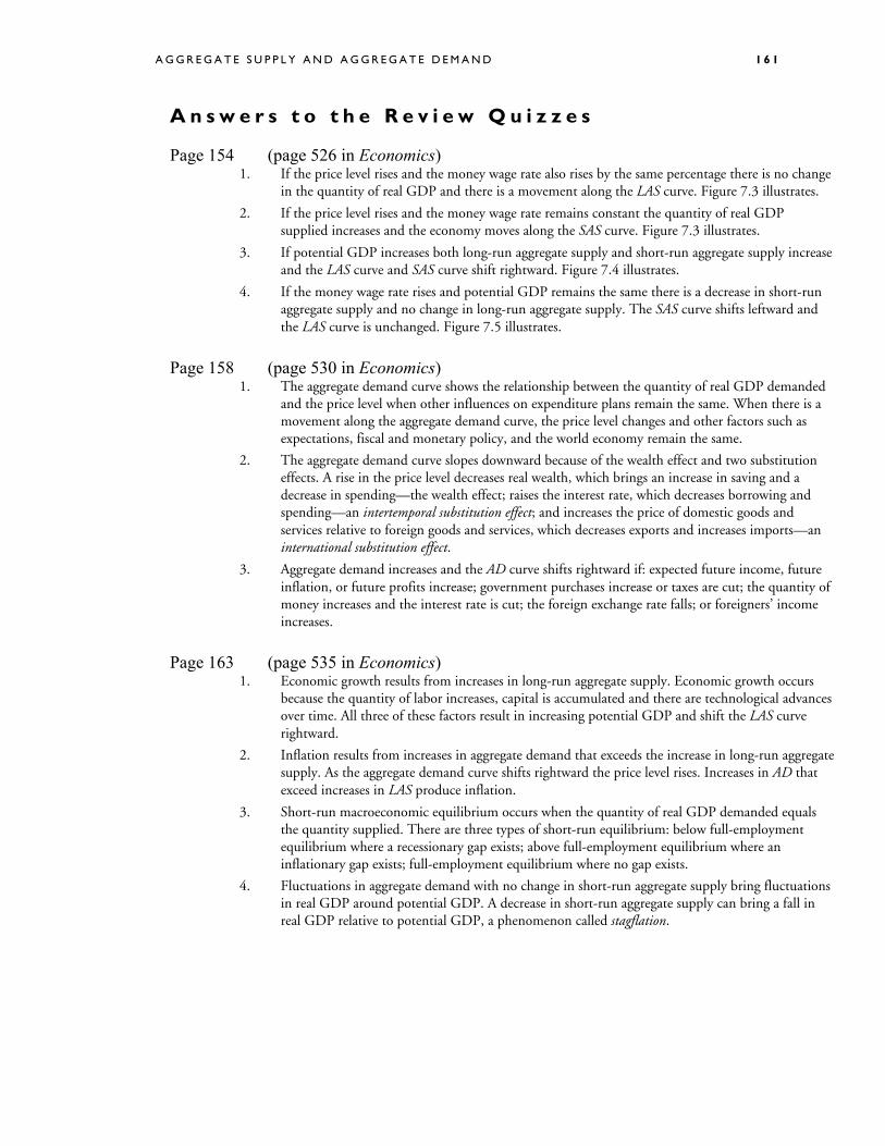
Page 154 (page 526 in Economics) 1. If the price level rises and the money wage rate also rises by the same percentage there is no change

in the quantity of real GDP and there is a movement along the LAS curve. Figure 7.3 illustrates.

2. If the price level rises and the money wage rate remains constant the quantity of real GDP supplied increases and the economy moves along the SAS curve. Figure 7.3 illustrates.

3. If potential GDP increases both long-run aggregate supply and short-run aggregate supply increase and the LAS curve and SAS curve shift rightward. Figure 7.4 illustrates.

4. If the money wage rate rises and potential GDP remains the same there is a decrease in short-run aggregate supply and no change in long-run aggregate supply. The SAS curve shifts leftward and the LAS curve is unchanged. Figure 7.5 illustrates.

Page 158 (page 530 in Economics) 1. The aggregate demand curve shows the relationship between the quantity of real GDP demanded

and the price level when other influences on expenditure plans remain the same. When there is a movement along the aggregate demand curve, the price level changes and other factors such as expectations, fiscal and monetary policy, and the world economy remain the same.

2. The aggregate demand curve slopes downward because of the wealth effect and two substitution effects. A rise in the price level decreases real wealth, which brings an increase in saving and a decrease in spending—the wealth effect; raises the interest rate, which decreases borrowing and spending—an intertemporal substitution effect; and increases the price of domestic goods and services relative to foreign goods and services, which decreases exports and increases imports—an international substitution effect.

3. Aggregate demand increases and the AD curve shifts rightward if: expected future income, future inflation, or future profits increase; government purchases increase or taxes are cut; the quantity of money increases and the interest rate is cut; the foreign exchange rate falls; or foreigners’ income increases.

Page 163 (page 535 in Economics) 1. Economic growth results from increases in long-run aggregate supply. Economic growth occurs

because the quantity of labor increases, capital is accumulated and there are technological advances over time. All three of these factors result in increasing potential GDP and shift the LAS curve rightward.

2. Inflation results from increases in aggregate demand that exceeds the increase in long-run aggregate supply. As the aggregate demand curve shifts rightward the price level rises. Increases in AD that exceed increases in LAS produce inflation.

3. Short-run macroeconomic equilibrium occurs when the quantity of real GDP demanded equals the quantity supplied. There are three types of short-run equilibrium: below full-employment equilibrium where a recessionary gap exists; above full-employment equilibrium where an inflationary gap exists; full-employment equilibrium where no gap exists.

4. Fluctuations in aggregate demand with no change in short-run aggregate supply bring fluctuations in real GDP around potential GDP. A decrease in short-run aggregate supply can bring a fall in real GDP relative to potential GDP, a phenomenon called stagflation.

1 6 2 C H A P T E R 7

A n s w e r s t o t h e P r o b l e m s 1. a A deep recession in the world economy decreases aggregate demand, which decreases real GDP

and lowers the price level. A sharp rise in oil prices decreases short-run aggregate supply, which decreases real GDP and raises the price level. The expectation of huge losses in the future decreases investment and decreases aggregate demand, which decreases real GDP and lowers the price level.

b. The combined effect of a deep recession in the world economy, a sharp rise in oil prices, and the expectation of huge losses in the future decreases both aggregate demand and short-run aggregate supply, which decreases real GDP and might raise or lower the price level.

c. The Toughtimes government might try to increase aggregate demand by increasing its purchases or by cutting taxes and the Toughtimes Fed might increase the quantity of money and lower interest rates. These policies could increase real GDP, but they would also raise the price level.

2. a. The strong expansion in the world economy increases Coolland’s exports and increases aggregate demand, which increases real GDP and raises the price level. The expectation of huge profits in the future increases investment and increases aggregate demand, which increases real GDP and raises the price level. A cut in government expenditures decreases aggregate demand, which decreases real GDP and lowers the price level.

b. The combined effect of a strong expansion in the world economy, the expectation of huge profits in the future, and a cut in government expenditures might increase of decrease aggregate demand, and so might increase or decreases real GDP and raise or lower the price level.

c. Coolland’s policymakers may be concerned about the net effect on Coolland’s economy. If the expansionary events dominate, Coolland’s government might want to take further contractionary actions (such as decreasing government purchases even more and/or raising taxes). Coolland’s Fed might want to decrease the quantity of money and raise interest rates. If the contractionary events dominate, then Coolland’s government may want to undertake expansionary policy (e.g., cut government spending less and/or cut taxes) and Coolland’s Fed may want to increase the money supply and lower interest rates.

3. a. Make a graph with the price level on the y-axis and real GDP on the x-axis. Make the price level values run from 80 to 150 in intervals of 10, and make the real GDP values run from 150 to 650 in intervals of 50. Plot the data in the table in the graph. The AD curve plots the price level against the quantity of real GDP demanded. The SAS curve plots the price level against the quantity of real GDP supplied in the short-run.

b. Equilibrium real GDP is $400 trillion and the price level is 100. Short-run macroeconomic equilibrium occurs at the intersection of the aggregate demand curve and the short-run aggregate supply curve.

c. The long-run aggregate supply curve is a vertical line in your graph at real GDP of $500 billion.

4. a. Make a graph with the price level on the y-axis and real GDP on the x-axis. Make the price level values run from 80 to 150 in intervals of 10, and make the real GDP values run from 50 to 650 in intervals of 50. Plot the data in the table in the graph. The AD curve plots the price level against the quantity of real GDP demanded. The SAS curve plots the price level against the quantity of real GDP supplied in the short-run.

b. Equilibrium real GDP is $300 trillion and the price level is 120. Short-run macroeconomic equilibrium occurs at the intersection of the aggregate demand curve and the short-run aggregate supply curve.

c. The long-run aggregate supply curve is a vertical line in your graph at real GDP of $250 billion.

5. Make a new table based on that in problem 3. Add a column headed “New real GDP demanded.” Enter values in this column that equal the value in the column headed “Real GDP demanded” plus $100 billion. (For example, on the first row of your new column, you have $550 billion.) Now, using

A G G R E G A T E S U P P L Y A N D A G G R E G A T E D E M A N D 1 6 3

the graph that you made to answer problem 3, add a new AD curve by plotting the price level against “New quantity of real GDP demanded.” The new equilibrium level of real GDP is $450 billion, and the price level is 110.

6. Make a new table based on that in problem 4. Add a column headed “New real GDP demanded.” Enter values in this column that equal the value in the column headed “Real GDP demanded” minus $150 billion. (For example, on the first row of your new column, you have $450 billion.) Now, using the graph that you made to answer problem 4, add a new AD curve by plotting the price level against “New quantity of real GDP demanded.” The new equilibrium level of real GDP is $250 billion, and the price level is 110.

7. Make a new table based on that in problem 3. Add a column headed “New real GDP supplied in the short run.” Enter values in this column that equal the value in the column headed “Real GDP supplied in the short run” minus $100 billion. (For example, on the first row of your new column, you have $250 billion.) Now, using the graph that you made to answer problem 3, add a new SAS curve by plotting the price level against “New quantity of real GDP supplied in the short run.” The new equilibrium level of real GDP is $350 billion, and the price level is 110.

8. Make a new table based on that in problem 4. Add a column headed “New real GDP supplied in the short run.” Enter values in this column that equal the value in the column headed “New real GDP supplied in the short run” plus $150 billion. (For example, on the first row of your new column, you have $300 billion.) Now, using the graph that you made to answer problem 4, add a new SAS curve by plotting the price level against “New quantity of real GDP supplied in the short run.” The new equilibrium level of real GDP is $400 billion, and the price level is 110.

9. a. Point C. The aggregate demand curve is the red curve AD1. The short-run aggregate supply curve is the blue curve SAS0. These curves intersect at point C.

b. Point D. The short-run aggregate supply curve is the red curve SAS1. The aggregate demand curve is now the red curve AD1. These curves intersect at point D.

c. Aggregate demand increases if (1) expected future incomes, inflation, or profits increase; (2) the government increases its purchases or reduces taxes; (3) the Fed increases the quantity of money and decreases interest rates; or (4) the exchange rate decreases or foreign income increases.

d. Short-run aggregate supply decreases if resource prices increase.

10. a. Point B. The short-run aggregate supply curve is SAS1. The aggregate demand curve has not changed. These curves intersect at point B.

b. There are three possible events that could have changed the long-run aggregate supply curve from LAS0 to LAS1: an increase in the full-employment quantity of labor; an increase in the quantity of capital; and/or an advance in technology.

c. The same events that changed the LAS curve also will shift the SAS curve. The SAS curve will shift by the same amount as the LAS curve.

d. After the increase in aggregate supply, there is a new short-run equilibrium at point B. Real GDP is less than potential GDP, which is now along the LAS1 curve. There is a recessionary gap at point B.

e. Aggregate demand would need to increase. Full-employment equilibrium would be achieved at point C with an increase in AD.