CHAPTER Introduction: Basic Principles 1 · Many textbooks, e.g., Çengel and Boles (1994),...

CHAPTER

Introduction: Basic Principles 1Take your choice of those that can best aid your action.

Shakespeare, Coriolanus

1.1 DEFINITION OF A TURBOMACHINEWe classify as turbomachines all those devices in which energy is transferred either to, or from, a con-tinuously flowing fluid by the dynamic action of one or more moving blade rows. The word turbo orturbinis is of Latin origin and implies that which spins or whirls around. Essentially, a rotating bladerow, a rotor or an impeller changes the stagnation enthalpy of the fluid moving through it by doingeither positive or negative work, depending upon the effect required of the machine. These enthalpychanges are intimately linked with the pressure changes occurring simultaneously in the fluid.

Two main categories of turbomachine are identified: firstly, those that absorb power to increase thefluid pressure or head (ducted and unducted fans, compressors, and pumps); secondly, those that pro-duce power by expanding fluid to a lower pressure or head (wind, hydraulic, steam, and gas turbines).Figure 1.1 shows, in a simple diagrammatic form, a selection of the many varieties of turbomachinesencountered in practice. The reason that so many different types of either pump (compressor) or turbineare in use is because of the almost infinite range of service requirements. Generally speaking, for a givenset of operating requirements one type of pump or turbine is best suited to provide optimum conditionsof operation.

Turbomachines are further categorised according to the nature of the flow path through the passagesof the rotor. When the path of the through-flow is wholly or mainly parallel to the axis of rotation, thedevice is termed an axial flow turbomachine [e.g., Figures 1.1(a) and (e)]. When the path of the through-flow is wholly or mainly in a plane perpendicular to the rotation axis, the device is termed a radial flowturbomachine [e.g., Figure 1.1(c)]. More detailed sketches of radial flow machines are given inFigures 7.3, 7.4, 8.2, and 8.3. Mixed flow turbomachines are widely used. The term mixed flow in thiscontext refers to the direction of the through-flow at the rotor outlet when both radial and axial velocitycomponents are present in significant amounts. Figure 1.1(b) shows amixed flow pump and Figure 1.1(d)a mixed flow hydraulic turbine.

One further category should be mentioned. All turbomachines can be classified as either impulse orreaction machines according to whether pressure changes are absent or present, respectively, in theflow through the rotor. In an impulse machine all the pressure change takes place in one or more noz-zles, the fluid being directed onto the rotor. The Pelton wheel, Figure 1.1(f), is an example of animpulse turbine.

© 2010 S. L. Dixon and C. A. Hall. Published by Elsevier Inc. All rights reserved.DOI: 10.1016/B978-1-85617-793-1.00001-8

1

The main purpose of this book is to examine, through the laws of fluid mechanics and thermo-dynamics, the means by which the energy transfer is achieved in the chief types of turbomachines,together with the differing behaviour of individual types in operation. Methods of analysing the flowprocesses differ depending upon the geometrical configuration of the machine, whether the fluid canbe regarded as incompressible or not, and whether the machine absorbs or produces work. As far aspossible, a unified treatment is adopted so that machines having similar configurations and functionare considered together.

1.2 COORDINATE SYSTEMTurbomachines consist of rotating and stationary blades arranged around a common axis, which meansthat they tend to have some form of cylindrical shape. It is therefore natural to use a cylindrical polarcoordinate system aligned with the axis of rotation for their description and analysis. This coordinate

(c) Centrifugal compressor or pump

Impeller

Volute

Vaneless diffuser

Outlet diffuser

Flow direction

(a) Single stage axial flow compressor or pump

Rotor bladesOutlet vanes

Flow

(e) Kaplan turbine

Draught tubeor diffuser

FlowFlow

Guide vanes

Rotor blades

Outlet vanesFlow

(b) Mixed flow pump

(d) Francis turbine (mixed flow type)

FlowFlow

Runner bladesGuide vanes

Draught tube

(f) Pelton wheel

WheelNozzle

Inlet pipe

Flow

Jet

FIGURE 1.1

Examples of Turbomachines

2 CHAPTER 1 Introduction: Basic Principles

system is pictured in Figure 1.2. The three axes are referred to as axial x, radial r, and tangential(or circumferential) rθ.

In general, the flow in a turbomachine has components of velocity along all three axes, which varyin all directions. However, to simplify the analysis it is usually assumed that the flow does not vary inthe tangential direction. In this case, the flow moves through the machine on axi symmetric streamsurfaces, as drawn on Figure 1.2(a). The component of velocity along an axi-symmetric stream surfaceis called the meridional velocity,

cm ¼ffiffiffiffiffiffiffiffiffiffiffiffiffiffic2x þ c2r

q. ð1:1Þ

In purely axial-flow machines the radius of the flow path is constant and therefore, referring toFigure 1.2(c) the radial flow velocity will be zero and cm ¼ cx. Similarly, in purely radial flow

cm

cx

cr

r

x Axis of rotation

Hub

Casing

Blade

Flow streamsurfaces

(a) Meridional or side view

(b) View along the axis (c) View looking down onto a stream surface

m

r�

cm

U

c

wc�

w��

�

r

r�

c�

V

U 5Vr

Hub

Casing

FIGURE 1.2

The Co-ordinate System and Flow Velocities within a Turbomachine

1.2 Coordinate System 3

machines the axial flow velocity will be zero and cm ¼ cr. Examples of both of these types ofmachines can be found in Figure 1.1.

The total flow velocity is made up of the meridional and tangential components and can be written

c ¼ffiffiffiffiffiffiffiffiffiffiffiffiffiffiffiffiffiffiffiffiffiffiffiffic2x þ c2r þ c2θ

q¼

ffiffiffiffiffiffiffiffiffiffiffiffiffiffiffic2m þ c2θ

q. ð1:2Þ

The swirl, or tangential, angle is the angle between the flow direction and the meridional direction:

α ¼ tan �1ðcθ=cmÞ. ð1:3Þ

Relative VelocitiesThe analysis of the flow-field within the rotating blades of a turbomachine is performed in a frame ofreference that is stationary relative to the blades. In this frame of reference the flow appears as steady,whereas in the absolute frame of reference it would be unsteady. This makes any calculations signi-ficantly more straightforward, and therefore the use of relative velocities and relative flow quantitiesis fundamental to the study of turbomachinery.

The relative velocity is simply the absolute velocity minus the local velocity of the blade. The bladehas velocity only in the tangential direction, and therefore the relative components of velocity can bewritten as

wθ ¼ cθ �U,wx ¼ cx,wr ¼ cr. ð1:4ÞThe relative flow angle is the angle between the relative flow direction and the meridional direction:

β ¼ tan �1ðwθ=cmÞ. ð1:5ÞBy combining eqns. (1.3), (1.4), and (1.5) a relationship between the relative and absolute flow anglescan be found:

tan β ¼ tan α�U=cm. ð1:6Þ

1.3 THE FUNDAMENTAL LAWSThe remainder of this chapter summarises the basic physical laws of fluid mechanics and thermo-dynamics, developing them into a form suitable for the study of turbomachines. Following this,some of the more important and commonly used expressions for the efficiency of compression andexpansion flow processes are given.

The laws discussed are

(i) the continuity of flow equation;(ii) the first law of thermodynamics and the steady flow energy equation;(iii) the momentum equation;(iv) the second law of thermodynamics.

All of these laws are usually covered in first-year university engineering and technology courses, soonly the briefest discussion and analysis is given here. Some textbooks dealing comprehensively


with these laws are those written by Çengel and Boles (1994); Douglas, Gasiorek, and Swaffield(1995); Rogers and Mayhew (1992); and Reynolds and Perkins (1977). It is worth rememberingthat these laws are completely general; they are independent of the nature of the fluid or whetherthe fluid is compressible or incompressible.

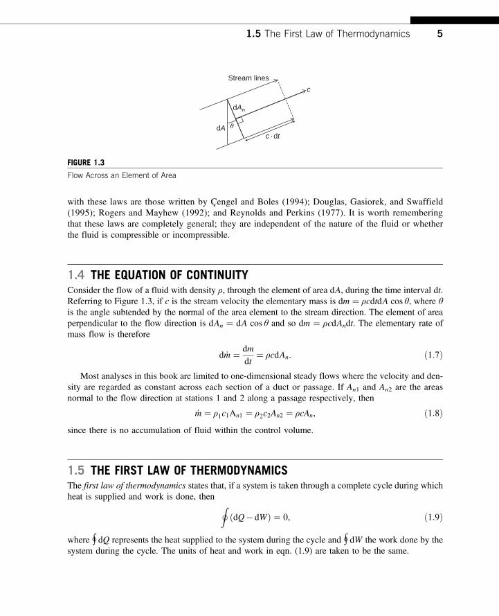
1.4 THE EQUATION OF CONTINUITYConsider the flow of a fluid with density ρ, through the element of area dA, during the time interval dt.Referring to Figure 1.3, if c is the stream velocity the elementary mass is dm ¼ ρcdtdA cos θ, where θis the angle subtended by the normal of the area element to the stream direction. The element of areaperpendicular to the flow direction is dAn ¼ dA cos θ and so dm ¼ ρcdAndt. The elementary rate ofmass flow is therefore

d _m ¼ dmdt

¼ ρcdAn. ð1:7Þ

Most analyses in this book are limited to one-dimensional steady flows where the velocity and den-sity are regarded as constant across each section of a duct or passage. If An1 and An2 are the areasnormal to the flow direction at stations 1 and 2 along a passage respectively, then

_m ¼ ρ1c1An1 ¼ ρ2c2An2 ¼ ρcAn, ð1:8Þsince there is no accumulation of fluid within the control volume.

1.5 THE FIRST LAW OF THERMODYNAMICSThe first law of thermodynamics states that, if a system is taken through a complete cycle during whichheat is supplied and work is done, then I

ðdQ� dWÞ ¼ 0, ð1:9Þ

where ∮ dQ represents the heat supplied to the system during the cycle and ∮ dW the work done by thesystem during the cycle. The units of heat and work in eqn. (1.9) are taken to be the same.

c

c · dt�

Stream lines

dAn

dA

FIGURE 1.3

Flow Across an Element of Area

1.5 The First Law of Thermodynamics 5

During a change from state 1 to state 2, there is a change in the energy within the system:

E2 �E1 ¼Z 2

1ðdQ� dWÞ, ð1:10aÞ

where E ¼U þ 12mc2 þmgz.

For an infinitesimal change of state,dE ¼ dQ� dW . ð1:10bÞ

The Steady Flow Energy EquationMany textbooks, e.g., Çengel and Boles (1994), demonstrate how the first law of thermodynamics isapplied to the steady flow of fluid through a control volume so that the steady flow energy equation isobtained. It is unprofitable to reproduce this proof here and only the final result is quoted. Figure 1.4shows a control volume representing a turbomachine, through which fluid passes at a steady rate ofmass flow _m, entering at position 1 and leaving at position 2. Energy is transferred from the fluidto the blades of the turbomachine, positive work being done (via the shaft) at the rate _Wx. In the generalcase positive heat transfer takes place at the rate _Q, from the surroundings to the control volume. Thus,with this sign convention the steady flow energy equation is

_Q� _Wx ¼ _m h2 � h1ð Þ þ 12ðc22 � c21Þ þ g z2 � z1ð Þ

� �, ð1:11Þ

where h is the specific enthalpy,12c2, the kinetic energy per unit mass and gz, the potential energy per

unit mass.For convenience, the specific enthalpy, h, and the kinetic energy,

12c2, are combined and the result

is called the stagnation enthalpy:

h0 ¼ hþ 12c2. ð1:12Þ

Apart from hydraulic machines, the contribution of the g(z2 � z1) term in eqn. (1.11) is small and canusually ignored. In this case, eqn. (1.11) can be written as

_Q� _Wx ¼ _mðh02 � h01Þ. ð1:13Þ

1

m

m2

Controlvolume

Q

Wx

FIGURE 1.4

Control Volume Showing Sign Convention for Heat and Work Transfers


The stagnation enthalpy is therefore constant in any flow process that does not involve a work transferor a heat transfer. Most turbomachinery flow processes are adiabatic (or very nearly so) and it is per-missible to write _Q ¼ 0. For work producing machines (turbines) _Wx > 0, so that

_Wx ¼ _Wt ¼ _mðh01� h02Þ. ð1:14ÞFor work absorbing machines (compressors) _Wx < 0, so that it is more convenient to write

_Wc ¼ � _Wx ¼ _mðh02 � h01Þ. ð1:15Þ

1.6 THE MOMENTUM EQUATIONOne of the most fundamental and valuable principles in mechanics is Newton’s second law of motion.The momentum equation relates the sum of the external forces acting on a fluid element to its accelera-tion, or to the rate of change of momentum in the direction of the resultant external force. In the studyof turbomachines many applications of the momentum equation can be found, e.g., the force exertedupon a blade in a compressor or turbine cascade caused by the deflection or acceleration of fluidpassing the blades.

Considering a system of mass m, the sum of all the body and surface forces acting on m along somearbitrary direction x is equal to the time rate of change of the total x-momentum of the system, i.e.,X

Fx ¼ ddtðmcxÞ. ð1:16aÞ

For a control volume where fluid enters steadily at a uniform velocity cx1 and leaves steadily with auniform velocity cx2, then X

Fx ¼ _mðcx2 � cx1Þ. ð1:16bÞEquation (1.16b) is the one-dimensional form of the steady flow momentum equation.

Moment of MomentumIn dynamics useful information can be obtained by employing Newton’s second law in the form whereit applies to the moments of forces. This form is of central importance in the analysis of the energytransfer process in turbomachines.

For a system of mass m, the vector sum of the moments of all external forces acting on the systemabout some arbitrary axis A–A fixed in space is equal to the time rate of change of angular momentumof the system about that axis, i.e.,

τΑ ¼ mddtðrcθÞ, ð1:17aÞ

where r is distance of the mass centre from the axis of rotation measured along the normal to the axisand cθ the velocity component mutually perpendicular to both the axis and radius vector r.

For a control volume the law of moment of momentum can be obtained. Figure 1.5 shows the con-trol volume enclosing the rotor of a generalised turbomachine. Swirling fluid enters the control volume

1.6 The Momentum Equation 7

at radius r1 with tangential velocity cθ1 and leaves at radius r2 with tangential velocity cθ2. For one-dimensional steady flow,

τA ¼ _mðr2cθ2 � r1cθ1Þ, ð1:17bÞwhich states that the sum of the moments of the external forces acting on fluid temporarily occupying thecontrol volume is equal to the net time rate of efflux of angular momentum from the control volume.

The Euler Work EquationFor a pump or compressor rotor running at angular velocity Ω, the rate at which the rotor does work onthe fluid is

τAΩ ¼ _mðU2cθ2 �U1cθ1Þ, ð1:18aÞwhere the blade speed U ¼ Ωr.

Thus, the work done on the fluid per unit mass or specific work is

ΔWc ¼_Wc

_m¼ τAΩ

_m¼ U2cθ2 �U1cθ1 > 0. ð1:18bÞ

This equation is referred to as Euler’s pump equation.For a turbine the fluid does work on the rotor and the sign for work is then reversed. Thus, the

specific work is

ΔWt ¼_Wt

_m¼ U1cθ1 �U2cθ2 > 0. ð1:18cÞ

Equation (1.18c) is referred to as Euler’s turbine equation.Note that, for any adiabatic turbomachine (turbine or compressor), applying the steady flow energy

equation, eqn. (1.13), gives

ΔWx ¼ ðh01 � h02Þ ¼ U1cθ1 �U2cθ2. ð1:19aÞAlternatively, this can be written as

Δh0 ¼ ΔðUcθÞ. ð1:19bÞ

�A, V

Flow direction

A A

r2r1

c�2

c�1

FIGURE 1.5

Control Volume for a Generalised Turbomachine


Equations (1.19a) and (1.19b) are the general forms of the Euler work equation. By considering theassumptions used in its derivation, this equation can be seen to be valid for adiabatic flow for anystreamline through the blade rows of a turbomachine. It is applicable to both viscous and inviscidflow, since the torque provided by the fluid on the blades can be exerted by pressure forces or frictionalforces. It is strictly valid only for steady flow but it can also be applied to time-averaged unsteady flowprovided the averaging is done over a long enough time period. In all cases, all of the torque from thefluid must be transferred to the blades. Friction on the hub and casing of a turbomachine can causelocal changes in angular momentum that are not accounted for in the Euler work equation.

Note that for any stationary blade row, U ¼ 0 and therefore h0 ¼ constant. This is to be expectedsince a stationary blade cannot transfer any work to or from the fluid.

Rothalpy and Relative VelocitiesThe Euler work equation, eqn. (1.19), can be rewritten as

I ¼ h0 �Ucθ, ð1:20aÞwhere I is a constant along the streamlines through a turbomachine. The function I has acquired thewidely used name rothalpy, a contraction of rotational stagnation enthalpy, and is a fluid mechanicalproperty of some importance in the study of flow within rotating systems. The rothalpy can also bewritten in terms of the static enthalpy as

I ¼ hþ 12c2 �Ucθ. ð1:20bÞ

The Euler work equation can also be written in terms of relative quantities for a rotating frame of reference.The relative tangential velocity, as given in eqn. (1.4), can be substituted in eqn. (1.20b) to produce

I ¼ hþ 12ðw2 þ U2 þ 2UwθÞ�Uðwθ þ UÞ ¼ hþ 1

2w2 � 1

2U2. ð1:21aÞ

Defining a relative stagnation enthalpy as h0,rel ¼ h þ 12w2, eqn. (1.21a) can be simplified to

I ¼ h0,rel � 12U2. ð1:21bÞ

This final form of the Euler work equation shows that, for rotating blade rows, the relative stagnationenthalpy is constant through the blades provided the blade speed is constant. In other words, h0,rel ¼constant, if the radius of a streamline passing through the blades stays the same. This result is importantfor analysing turbomachinery flows in the relative frame of reference.

1.7 THE SECOND LAW OF THERMODYNAMICS—ENTROPYThe second law of thermodynamics, developed rigorously in many modern thermodynamic textbooks,e.g., Çengel and Boles (1994), Reynolds and Perkins (1977), and Rogers and Mayhew (1992), enablesthe concept of entropy to be introduced and ideal thermodynamic processes to be defined.

1.7 The Second Law of Thermodynamics—Entropy 9

An important and useful corollary of the second law of thermodynamics, known as the inequality ofClausius, states that, for a system passing through a cycle involving heat exchanges,I

dQT

≤ 0, ð1:22aÞ

where dQ is an element of heat transferred to the system at an absolute temperature T. If all the pro-cesses in the cycle are reversible, then dQ ¼ dQR, and the equality in eqn. (1.22a) holds true, i.e.,I

dQR

T¼ 0: ð1:22bÞ

The property called entropy, for a finite change of state, is then defined as

S2 � S1 ¼Z 2

1

dQR

T. ð1:23aÞ

For an incremental change of state

dS ¼ mds ¼ dQR

T, ð1:23bÞ

where m is the mass of the system.With steady one-dimensional flow through a control volume in which the fluid experiences a

change of state from condition 1 at entry to 2 at exit,Z 2

1

d _QT

≤ _mðs2 � s1Þ. ð1:24aÞ

Alternatively, this can be written in terms of an entropy production due to irreversibility, ΔSirrev:

_mðs2 � s1Þ ¼Z 2

1

d _QT

þ ΔSirrev. ð1:24bÞ

If the process is adiabatic, d _Q ¼ 0, then

s2 ≥ s1. ð1:25ÞIf the process is reversible as well, then

s2 ¼ s1. ð1:26ÞThus, for a flow undergoing a process that is both adiabatic and reversible, the entropy will remainunchanged (this type of process is referred to as isentropic). Since turbomachinery is usually adiabatic,or close to adiabatic, an isentropic compression or expansion represents the best possible process thatcan be achieved. To maximize the efficiency of a turbomachine, the irreversible entropy productionΔSirrev must be minimized, and this is a primary objective of any design.

Several important expressions can be obtained using the preceding definition of entropy. For a systemof mass m undergoing a reversible process dQ¼ dQR¼mTds and dW¼ dWR¼mpdv. In the absence ofmotion, gravity, and other effects the first law of thermodynamics, eqn. (1.10b) becomes

Tds ¼ duþ pdv. ð1:27Þ


With h¼ uþ pv, then dh¼ duþ pdvþ vdp, and eqn. (1.27) then gives

Tds ¼ dh� vdp. ð1:28ÞEquations (1.27) and (1.28) are extremely useful forms of the second law of thermodynamics

because the equations are written only in terms of properties of the system (there are no terms involvingQ or W ). These equations can therefore be applied to a system undergoing any process.

Entropy is a particularly useful property for the analysis of turbomachinery. Any creation ofentropy in the flow path of a machine can be equated to a certain amount of “lost work” and thus aloss in efficiency. The value of entropy is the same in both the absolute and relative frames of reference(see Figure 1.7 later) and this means it can be used to track the sources of inefficiency through all therotating and stationary parts of a machine. The application of entropy to account for lost performance isvery powerful and will be demonstrated in later sections.

1.8 BERNOULLI’S EQUATIONConsider the steady flow energy equation, eqn. (1.11). For adiabatic flow, with no work transfer,

ðh2 � h1Þ þ 12ðc22 � c21Þ þ g z2 � z1ð Þ ¼ 0. ð1:29Þ

If this is applied to a control volume whose thickness is infinitesimal in the stream direction(Figure 1.6), the following differential form is derived:

dhþ cdcþ gdz ¼ 0: ð1:30ÞIf there are no shear forces acting on the flow (no mixing or friction), then the flow will be isentropicand, from eqn. (1.28), dh¼ vdp¼ dp/ρ, giving

1ρdpþ cdcþ gdz ¼ 0: ð1:31aÞ

Fluid density, �

Fixed datum

ZZ 1dZ

2

1

cc 1dc

p1dp

p

Streamflow

FIGURE 1.6

Control Volume in a Streaming Fluid

1.8 Bernoulli’s Equation 11

Equation (1.31) is often referred to as the one-dimensional form of Euler’s equation of motion. Inte-grating this equation in the stream direction we obtainZ 2

1

1ρdpþ 1

2ðc22 � c21Þ þ gðz2 � z1Þ ¼ 0, ð1:31bÞ

which is Bernoulli’s equation. For an incompressible fluid, ρ is constant and eqn. (1.31b) becomes

1ρ

p02 � p01ð Þ þ g z2 � z1ð Þ ¼ 0, ð1:31cÞ

where the stagnation pressure for an incompressible fluid is p0 ¼ pþ 12ρc2.

When dealing with hydraulic turbomachines, the term head, H, occurs frequently and describes thequantity z þ p0/( ρg). Thus, eqn. (1.31c) becomes

H2 �H1 ¼ 0. ð1:31dÞIf the fluid is a gas or vapour, the change in gravitational potential is generally negligible and eqn.

(1.31b) is then Z 2

1

1ρdpþ 1

2ðc22 � c21Þ ¼ 0. ð1:31eÞ

Now, if the gas or vapour is subject to only small pressure changes the fluid density is sensibly constantand integration of eqn. (1.31e) gives

p02 ¼ p01 ¼ p0, ð1:31fÞi.e., the stagnation pressure is constant (it is shown later that this is also true for a compressible isen-tropic process).

1.9 COMPRESSIBLE FLOW RELATIONSThe Mach number of a flow is defined as the velocity divided by the local speed of sound. For a perfectgas, such as air, the Mach number can be written as

M ¼ c

a¼ cffiffiffiffiffiffiffiffi

γRTp . ð1:32Þ

Whenever the Mach number in a flow exceeds about 0.3, the flow becomes compressible, and thefluid density can no longer be considered as constant. High power turbomachines require high flowrates and high blade speeds and this inevitably leads to compressible flow. The static and stagnationquantities in the flow can be related using functions of the local Mach number and these are derived later.

Starting with the definition of stagnation enthalpy, h0 ¼ h þ 12c2, this can be rewritten for a perfect

gas as

CpT0 ¼ CpT þ c2

2¼ CpT þM2γRT

2. ð1:33aÞ


Given that γR ¼ (γ � 1)CP, eqn. (1.33a) can be simplified to

T0T

¼ 1þ γ� 12

M2. ð1:33bÞ

The stagnation pressure in a flow is the static pressure that is measured if the flow is brought isen-tropically to rest. From eqn. (1.28), for an isentropic process dh ¼ dp/ρ. If this is combined with theequation of state for a perfect gas, p ¼ ρRT, the following equation is obtained:

dpp

¼ Cp

R

dTT

¼ dTT

γγ� 1

ð1:34Þ

This can be integrated between the static and stagnation conditions to give the following compressibleflow relation between the stagnation and static pressure:

p0p¼ T0

T

� �γ=ðγ�1Þ¼ 1þ γ� 1

2M2

� �γ=ðγ�1Þ. ð1:35Þ

Equation (1.34) can also be integrated along a streamline between any two arbitrary points 1 and 2within an isentropic flow. In this case, the stagnation temperatures and pressures are related:

p02p01

¼ T02T01

� �γ=ðγ�1Þ. ð1:36Þ

If there is no heat or work transfer to the flow, T0 ¼ constant. Hence, eqn. (1.36) shows that, in isen-tropic flow with no work transfer, p02 ¼ p01 ¼ constant, which was shown to be the case for incom-pressible flow in eqn. (1.31f).

Combining the equation of state, p ¼ ρRT with eqns. (1.33b) and (1.35) the corresponding relation-ship for the stagnation density is obtained:

ρ0ρ¼ 1þ γ� 1

2M2

� �1=ðγ�1Þ. ð1:37Þ

Arguably the most important compressible flow relationship for turbomachinery is the one fornon-dimensional mass flow rate, sometimes referred to as capacity. It is obtained by combiningeqns. (1.33b), (1.35), and (1.37) with continuity, eqn. (1.8):

_mffiffiffiffiffiffiffiffiffiffiffiCPT0

pAnp0

¼ γffiffiffiffiffiffiffiffiffiffiγ� 1

p M 1þ γ� 12

M2

� �� 12

γþ1γ�1

� �. ð1:38Þ

This result is important since it can be used to relate the flow properties at different points within acompressible flow turbomachine. The application of eqn. (1.38) is demonstrated in Chapter 3.

Note that the compressible flow relations given previously can be applied in the relative frame ofreference for flow within rotating blade rows. In this case relative stagnation properties and relativeMach numbers are used:

p0,relp

,T0,relT

,ρ0,relρ

,_m

ffiffiffiffiffiffiffiffiffiffiffiffiffiffiCpT0,rel

pAp0,rel

¼ f ðMrelÞ. ð1:39Þ

1.9 Compressible Flow Relations 13

Figure 1.7 shows the relationship between stagnation and static conditions on a temperature–entropydiagram, in which the temperature differences have been exaggerated for clarity. This shows the relativestagnation properties as well as the absolute properties for a single point in a flow. Note that all of theconditions have the same entropy because the stagnation states are defined using an isentropic process.The pressures and temperatures are related using eqn. (1.35).

s0080 Variation of Gas Properties with TemperatureThe thermodynamic properties of a gas, Cp and γ, are dependent upon its temperature level, and someaccount must be taken of this effect. To illustrate this dependency the variation in the values of Cp andγ with the temperature for air are shown in Figure 1.8. In the calculation of expansion or compressionprocesses in turbomachines the normal practice is to use weighted mean values for Cp and γ accordingto the mean temperature of the process. Accordingly, in all problems in this book values have beenselected for Cp and γ appropriate to the gas and the temperature range.

T

s

p01

p 5 p1T1

T01

s1

c 2/(2Cp)

w 2/(2Cp)

1

01

p01,rel01,rel

T01,rel

FIGURE 1.7

Relationship Between Stagnation and Static Quantities on a Temperature–Entropy Diagram

600 1000 1400 1800

1.3

1.35

1.41.2

1.1

1.0

Cp

Cp

kJ/(

kgK

)

200

� �

FIGURE 1.8

Variation of Gas Properties with Temperature for Dry Air (data from Rogers and Mayhew, 1995)


1.10 DEFINITIONS OF EFFICIENCYA large number of efficiency definitions are included in the literature of turbomachines and mostworkers in this field would agree there are too many. In this book only those considered to be importantand useful are included.

Efficiency of TurbinesTurbines are designed to convert the available energy in a flowing fluid into useful mechanical workdelivered at the coupling of the output shaft. The efficiency of this process, the overall efficiency η0, isa performance factor of considerable interest to both designer and user of the turbine. Thus,

η0 ¼mechanical energy available at coupling of output shaft in unit time

maximum energy difference possible for the fluid in unit time.

Mechanical energy losses occur between the turbine rotor and the output shaft coupling as a resultof the work done against friction at the bearings, glands, etc. The magnitude of this loss as a fraction ofthe total energy transferred to the rotor is difficult to estimate as it varies with the size and individualdesign of turbomachine. For small machines (several kilowatts) it may amount to 5% or more, but formedium and large machines this loss ratio may become as little as 1%. A detailed consideration of themechanical losses in turbomachines is beyond the scope of this book and is not pursued further.

The isentropic efficiency ηt or hydraulic efficiency ηh for a turbine is, in broad terms,

ηt ðor ηhÞ ¼mechanical energy supplied to the rotor in unit time

maximum energy difference possible for the fluid in unit time.

Comparing these definitions it is easily deduced that the mechanical efficiency ηm, which is simply theratio of shaft power to rotor power, is

ηm ¼ η0=ηt ðor η0=ηhÞ. ð1:40ÞThe preceding isentropic efficiency definition can be concisely expressed in terms of the work done bythe fluid passing through the turbine:

ηt ðor ηhÞ ¼actual work

ideal ðmaximumÞ work ¼ ΔWx

ΔWmax. ð1:41Þ

The actual work is unambiguous and straightforward to determine from the steady flow energy equa-tion, eqn. (1.11). For an adiabatic turbine, using the definition of stagnation enthalpy,

ΔWx ¼ _Wx= _m ¼ ðh01 � h02Þ þ gðz1 � z2Þ.The ideal work is slightly more complicated as it depends on how the ideal process is defined. Theprocess that gives maximum work will always be an isentropic expansion, but the question is oneof how to define the exit state of the ideal process relative to the actual process. In the following para-graphs the different definitions are discussed in terms of to what type of turbine they are applied.

1.10 Definitions of Efficiency 15

Steam and Gas TurbinesFigure 1.9(a) shows a Mollier diagram representing the expansion process through an adiabatic turbine.Line 1–2 represents the actual expansion and line 1–2s the ideal or reversible expansion. The fluidvelocities at entry to and exit from a turbine may be quite high and the corresponding kinetic energiessignificant. On the other hand, for a compressible fluid the potential energy terms are usually negligible.Hence, the actual turbine rotor specific work is

ΔWx ¼ _Wx= _m ¼ h01 � h02 ¼ ðh1 � h2Þ þ 12ðc21 � c22Þ.

There are two main ways of expressing the isentropic efficiency, the choice of definition dependinglargely upon whether the exit kinetic energy is usefully employed or is wasted. If the exhaust kineticenergy is useful, then the ideal expansion is to the same stagnation (or total) pressure as the actualprocess. The ideal work output is therefore that obtained between state points 01 and 02s,

ΔWmax ¼ _Wmax= _m ¼ h01 � h02s ¼ ðh1 � h2sÞ þ 12ðc21 � c22sÞ.

The relevant adiabatic efficiency, η, is called the total-to-total efficiency and it is given by

ηtt ¼ ΔWx=ΔWmax ¼ ðh01 � h02Þ=ðh01 � h02sÞ. ð1:42aÞ

If the difference between the inlet and outlet kinetic energies is small, i.e.,12c21 @

12c22, then

ηtt ¼ ðh1 � h2Þ=ðh1 � h2sÞ. ð1:42bÞAn example where the exhaust kinetic energy is not wasted is from the last stage of an aircraft gasturbine where it contributes to the jet propulsive thrust. Likewise, the exit kinetic energy from onestage of a multistage turbine where it can be used in the following stage provides another example.

h

ss1 s2

h

(a) Turbine expansion process (b) Compression process

ss1 s2

21 2c1

21 2c1

21 2c2s

21 2c2s

21 2c2

21 2c2

02s

02

2s

02s

2s

2

02

2

01

1

01

1

p01

p01

p1

p1

p02

p02

p2

p2

FIGURE 1.9

Enthalpy–Entropy Diagrams for the Flow Through an Adiabatic Turbine and an Adiabatic Compressor


If, instead, the exhaust kinetic energy cannot be usefully employed and is entirely wasted, the idealexpansion is to the same static pressure as the actual process with zero exit kinetic energy. The idealwork output in this case is that obtained between state points 01 and 2s:

ΔWmax ¼ _Wmax= _m ¼ h01 � h2s ¼ ðh1 � h2sÞ þ 12c21.

The relevant adiabatic efficiency is called the total-to-static efficiency ηts and is given by

ηts ¼ ΔWx=ΔWmax ¼ ðh01 � h02Þ=ðh01 � h2sÞ. ð1:43aÞIf the difference between inlet and outlet kinetic energies is small, eqn. (1.43a) becomes

ηts ¼ h1 � h2ð Þ.

h1 � h2s þ 12c21

� �. ð1:43bÞ

A situation where the outlet kinetic energy is wasted is a turbine exhausting directly to the surround-ings rather than through a diffuser. For example, auxiliary turbines used in rockets often have noexhaust diffusers because the disadvantages of increased mass and space utilisation are greater thanthe extra propellant required as a result of reduced turbine efficiency.

By comparing eqns. (1.42) and (1.43) it is clear that the total-to-static efficiency will always belower than the total-to-total efficiency. The total-to-total efficiency relates to the internal losses(entropy creation) within the turbine, whereas the total-to-static efficiency relates to the internal lossesplus the wasted kinetic energy.

Hydraulic TurbinesThe turbine hydraulic efficiency is a form of the total-to-total efficiency expressed previously. Thesteady flow energy equation (eqn. 1.11) can be written in differential form for an adiabatic turbine as

d _Wx ¼ _m dhþ 12dðc2Þ þ gdz

� �.

For an isentropic process, Tds¼ 0¼ dh� dp/ρ. The maximumwork output for an expansion to the sameexit static pressure, kinetic energy, and height as the actual process is therefore

_Wmax ¼ _m

Z 2

1

1ρdpþ 1

2ðc21 � c22Þ þ gðz1 � z2Þ

� �.

For an incompressible fluid, the maximum work output from a hydraulic turbine (ignoring frictionallosses) can be written

_Wmax ¼ _m1ρðp1 � p2Þ þ 1

2ðc21 � c22Þ þ gðz1 � z2Þ

� �¼ _mgðH1 �H2Þ,

where gH ¼ p/ρþ 12c2þ gz and _m ¼ ρQ.

The turbine hydraulic efficiency, ηh, is the work supplied by the rotor divided by the hydrodynamicenergy difference of the fluid, i.e.,

ηh ¼_Wx

_Wmax¼ ΔWx

g H1 �H2½ � . ð1:44Þ

1.10 Definitions of Efficiency 17

Efficiency of Compressors and PumpsThe isentropic efficiency, ηc, of a compressor or the hydraulic efficiency of a pump, ηh, is broadlydefined as

ηc ðor ηhÞ ¼useful ðhydrodynamicÞ energy input to fluid in unit time

power input to rotor

The power input to the rotor (or impeller) is always less than the power supplied at the couplingbecause of external energy losses in the bearings, glands, etc. Thus, the overall efficiency of the com-pressor or pump is

ηo ¼useful ðhydrodynamicÞ energy input to fluid in unit time

power input to coupling of shaft.

Hence, the mechanical efficiency is

ηm ¼ ηo=ηc ðor ηo=ηhÞ. ð1:45ÞFor a complete adiabatic compression process going from state 1 to state 2, the specific work input is

ΔWc ¼ ðh02 � h01Þ þ gðz2 � z1Þ.Figure 1.9(b) shows a Mollier diagram on which the actual compression process is represented by thestate change 1–2 and the corresponding ideal process by 1–2s. For an adiabatic compressor in whichpotential energy changes are negligible, the most meaningful efficiency is the total-to-total efficiency,which can be written as

ηc ¼ideal ðminimumÞwork input

actual work input¼ h02s � h01

h02 � h01. ð1:46aÞ

If the difference between inlet and outlet kinetic energies is small,12c21 @

12c22 then

ηc ¼h2s � h1h2 � h1

. ð1:46bÞ

For incompressible flow, the minimum work input is given by

ΔWmin ¼ _Wmin= _m¼ ð p2 � p1Þ=ρþ 12ðc22 � c21Þ þ gðz2 � z1Þ

� �¼ g½H2 �H1�.

For a pump the hydraulic efficiency is therefore defined as

ηh ¼_Wmin

_Wc¼ g½H2 �H1�

ΔWc. ð1:47Þ

1.11 SMALL STAGE OR POLYTROPIC EFFICIENCYThe isentropic efficiency described in the preceding section, although fundamentally valid, can be mis-leading if used for comparing the efficiencies of turbomachines of differing pressure ratios. Now, anyturbomachine may be regarded as being composed of a large number of very small stages, irrespective


of the actual number of stages in the machine. If each small stage has the same efficiency, then theisentropic efficiency of the whole machine will be different from the small stage efficiency, the differ-ence depending upon the pressure ratio of the machine. This perhaps rather surprising result is a mani-festation of a simple thermodynamic effect concealed in the expression for isentropic efficiency and ismade apparent in the following argument.

Compression ProcessFigure 1.10 shows an enthalpy–entropy diagram on which adiabatic compression between pressures p1and p2 is represented by the change of state between points 1 and 2. The corresponding reversible pro-cess is represented by the isentropic line 1 to 2s. It is assumed that the compression process may bedivided into a large number of small stages of equal efficiency ηp. For each small stage the actualwork input is δW and the corresponding ideal work in the isentropic process is δWmin. With the nota-tion of Figure 1.10,

ηp ¼δWmin

δW¼ hxs � h1

hx � h1¼ hys � hx

hy � hx¼ � � �

Since each small stage has the same efficiency, then ηp¼ (ΣδWmin /ΣδW ) is also true.From the relation Tds ¼ dh – vdp, for a constant pressure process, (∂h/∂s)p1 ¼ T. This means that

the higher the fluid temperature, the greater is the slope of the constant pressure lines on the Mollierdiagram. For a gas where h is a function of T, constant pressure lines diverge and the slope of the line

Angles equal

s

h

2s

ys

y

Xs

X

1

p 2

p 1

p

2

FIGURE 1.10

Compression Process by Small Stages

1.11 Small Stage or Polytropic Efficiency 19

p2 is greater than the slope of line p1 at the same value of entropy. At equal values of T, constantpressure lines are of equal slope as indicated in Figure 1.10. For the special case of a perfect gas(where Cp is constant), Cp(dT/ds) ¼ T for a constant pressure process. Integrating this expressionresults in the equation for a constant pressure line, s ¼ Cp logT þ constant.

Returning now to the more general case, since

ΣdW ¼ fðhx � h1Þ þ ðhy � hxÞ þ � � �g ¼ ðh2 � h1Þ,then

ηp ¼ðhxs � h1Þ þ ðhys � hxÞ þ � � �=ðh2 � h1Þ.

The adiabatic efficiency of the whole compression process is

ηc ¼ ðh2s � h1Þ=ðh2 � h1Þ.Due to the divergence of the constant pressure lines

fðhxs � h1Þ þ ðhys � hxÞ þ � � �g> ðh2s � h1Þ,i.e.,

ΣδWmin >Wmin.

Therefore,

ηp > ηc.

Thus, for a compression process the isentropic efficiency of the machine is less than the small stageefficiency, the difference being dependent upon the divergence of the constant pressure lines. Althoughthe foregoing discussion has been in terms of static states it also applies to stagnation states since theseare related to the static states via isentropic processes.

Small Stage Efficiency for a Perfect GasAn explicit relation can be readily derived for a perfect gas (Cp is constant) between small stage effi-ciency, the overall isentropic efficiency and the pressure ratio. The analysis is for the limiting case ofan infinitesimal compressor stage in which the incremental change in pressure is dp as indicated inFigure 1.11. For the actual process the incremental enthalpy rise is dh and the corresponding idealenthalpy rise is dhis.

The polytropic efficiency for the small stage is

ηp ¼dhisdh

¼ vdpCpdT

, ð1:48Þ

since for an isentropic process Tds ¼ 0 ¼ dhis � vdp. Substituting v ¼ RT/p into eqn. (1.48) and usingCp ¼ γR/(γ� 1) gives

dTT

¼ ðγ� 1Þγηp

dpp. ð1:49Þ


Integrating eqn. (1.49) across the whole compressor and taking equal efficiency for each infinitesimalstage gives

T2T1

¼ p2p1

� �ðγ�1Þ=ηpγ. ð1:50Þ

Now the isentropic efficiency for the whole compression process is

ηc ¼ ðT2s � T1Þ=ðT2 � T1Þ ð1:51Þ

if it is assumed that the velocities at inlet and outlet are equal.For the ideal compression process put ηp¼ 1 in eqn. (1.50) and so obtain

T2sT1

¼ p2p1

� �ðγ�1Þ=γ, ð1:52Þ

which is equivalent to eqn. (1.36). Substituting eqns. (1.50) and (1.52) into eqn. (1.51) results in theexpression

ηc ¼p2p1

� �ðγ�1Þ=γ� 1

" #p2p1

� �ðγ�1Þ=ηpγ� 1

" #.

,ð1:53Þ

Values of “overall” isentropic efficiency have been calculated using eqn. (1.53) for a range of pressureratio and different values of ηp; these are plotted in Figure 1.12. This figure amplifies the observationmade earlier that the isentropic efficiency of a finite compression process is less than the efficiency ofthe small stages. Comparison of the isentropic efficiency of two machines of different pressure ratios isnot a valid procedure since, for equal polytropic efficiency, the compressor with the higher pressureratio is penalised by the hidden thermodynamic effect.

h

s

p

p1dp

dhdhis

FIGURE 1.11

Incremental Change of State in a Compression Process


Example 1.1An axial flow air compressor is designed to provide an overall total-to-total pressure ratio of 8 to 1. At inlet andoutlet the stagnation temperatures are 300 K and 586.4 K, respectively.

Determine the overall total-to-total efficiency and the polytropic efficiency for the compressor. Assume that γfor air is 1.4.

SolutionFrom eqn. (1.46), substituting h¼CpT, the efficiency can be written as

ηC ¼ T02s � T01T02 � T01

¼p02p01

� �ðγ�1Þ=γ� 1

T02=T01 � 1¼ 81=3.5 � 1

586� 4=300� 1¼ 0.85.

From eqn. (1.50), taking logs of both sides and rearranging, we get

ηp¼γ� 1γ

lnðp02=p01ÞlnðT02=T01Þ ¼

13:5

� ln 8ln 1:9547

¼ 0:8865:

Turbine Polytropic EfficiencyA similar analysis to the compression process can be applied to a perfect gas expanding through an adiabaticturbine. For the turbine the appropriate expressions for an expansion, from a state 1 to a state 2, are

Pressure ratio, p2 /p1

1 2 3 4 5 6 7 8 9

0.7

0.8

0.8

0.7Is

entr

opic

effi

cien

cy, �

c

0.6

0.9�p5 0.9

FIGURE 1.12

Relationship Between Isentropic (Overall) Efficiency, Pressure Ratio, and Small Stage (Polytropic) Efficiency for aCompressor (γ = 1.4)


T2T1

¼ p2p1

� �ηpðγ�1Þ=γ, ð1:54Þ

ηt ¼ 1� p2p1

� �ηpðγ�1Þ=γ" #1� p2

p1

� �ðγ�1Þ=γ" #.

,ð1:55Þ

The derivation of these expressions is left as an exercise for the student. “Overall” isentropic effi-ciencies have been calculated for a range of pressure ratios and polytropic efficiencies, and these areshown in Figure 1.13. The most notable feature of these results is that, in contrast with a compressionprocess, for an expansion, isentropic efficiency exceeds small stage efficiency.

Reheat FactorThe foregoing relations cannot be applied to steam turbines as vapours do not obey the perfect gaslaws. It is customary in steam turbine practice to use a reheat factor RH as a measure of the inefficiencyof the complete expansion. Referring to Figure 1.14, the expansion process through an adiabatic tur-bine from state 1 to state 2 is shown on a Mollier diagram, split into a number of small stages. Thereheat factor is defined as

RH ¼ ðh1 � hxsÞ þ ðhx � hysÞ þ � � �=ðh1 � h2sÞ ¼ ðΣΔhisÞ=ðh1 � h2sÞ.Due to the gradual divergence of the constant pressure lines on a Mollier chart, RH is always greaterthan unity. The actual value of RH for a large number of stages will depend upon the position of theexpansion line on the Mollier chart and the overall pressure ratio of the expansion. In normal steamturbine practice the value of RH is usually between 1.03 and 1.08.

Pressure ratio, p1 /p2

1 2 3 4 5 6 7 8 9

0.8

0.7

0.6

0.8

0.7Is

entr

opic

effi

cien

cy, �

t

0.6

0.9

�p5 0.9

FIGURE 1.13

Turbine Isentropic Efficiency against Pressure Ratio for Various Polytropic Efficiencies (γ = 1.4)


Now since the isentropic efficiency of the turbine is

ηt ¼h1 � h2h1 � h2s

¼ h1 � h2ΣΔhis

� ΣΔhish1 � h2s

,

then

ηt ¼ ηpRH , ð1:56Þwhich establishes the connection between polytropic efficiency, reheat factor and turbine isentropicefficiency.

1.12 THE INHERENT UNSTEADINESS OF THE FLOW WITHINTURBOMACHINES

It is a less well-known fact often ignored by designers of turbomachinery that turbomachines can onlywork the way they do because of flow unsteadiness. This subject was discussed by Dean (1959),Horlock and Daneshyar (1970), and Greitzer (1986). Here, only a brief introduction to an extensivesubject is given.

1

Dhis

xs

ys

y

z

xDh

h

s

p 2

p 1

2s

2

FIGURE 1.14

Mollier Diagram Showing Expansion Process Through a Turbine Split up into a Number of Small Stages


In the absence of viscosity, the equation for the stagnation enthalpy change of a fluid particlemoving through a turbomachine is

Dh0Dt

¼ 1ρ∂p∂t

, ð1:57Þ

where D/Dt is the rate of change following the fluid particle. Eqn. (1.57) shows us that any change instagnation enthalpy of the fluid is a result of unsteady variations in static pressure. In fact, withoutunsteadiness, no change in stagnation enthalpy is possible and thus no work can be done by thefluid. This is the so-called “Unsteadiness Paradox.” Steady approaches can be used to determinethe work transfer in a turbomachine, yet the underlying mechanism is fundamentally unsteady.

A physical situation considered by Greitzer is the axial compressor rotor as depicted in Figure 1.15a.The pressure field associated with the blades is such that the pressure increases from the suction surface(S) to the pressure surface (P). This pressure field moves with the blades and is therefore steady in therelative frame of reference. However, for an observer situated at the point* (in the absolute frame ofreference), a pressure that varies with time would be recorded, as shown in Figure 1.15b. This unsteadypressure variation is directly related to the blade pressure field via the rotational speed of the blades,

∂p∂t

¼ Ω∂p∂θ

¼ U∂pr∂θ

. ð1:58Þ

Thus, the fluid particles passing through the rotor experience a positive pressure increase with time(i.e., ∂p/∂t > 0) and their stagnation enthalpy is increased.

*

P

S

Dire

ctio

n of

bla

de m

otio

n

Sta

tic p

ress

ure

at *

Time(b)

(a)

Locationof statictapping

FIGURE 1.15

Measuring the Unsteady Pressure Field of an Axial Compressor Rotor: (a) Pressure Measured at Point* on theCasing, (b) Fluctuating Pressure Measured at Point*

1.12 The Inherent Unsteadiness of the Flow Within Turbomachines 25

ReferencesÇengel, Y. A., and Boles, M. A. (1994). Thermodynamics: An Engineering Approach (2nd ed.). New York:

McGraw-Hill.Dean, R. C. (1959). On the necessity of unsteady flow in fluid mechanics. Journal of Basic Engineering, Transactions of

the American Society of Mechanical Engineers, 81, 24–28.Denton, J. D. (1993). Loss mechanisms in turbomachines. J. Turbomachinery, Transactions of the American Society of

Mechanical Engineers, 115(4), 621–656.Douglas, J. F., Gasioreck, J. M., and Swaffield, J. A. (1995). Fluid Mechanics. New York: Longman.Greitzer, E. M. (1986). An introduction to unsteady flow in turbomachines. In D. Japikse (ed.), Advanced Topics in

Turbomachinery, Principal Lecture Series No. 2 (Concepts ETI.)Horlock, J. H. (1966). Axial Flow Turbines. London: Butterworth. (1973 reprint with corrections, Huntington, NY:

Krieger.)Horlock, J. H., and Daneshyar, H. (1970). Stagnation pressure changes in unsteady flow. Aeronautical Quarterly, 22,

207–224.Reynolds, C., and Perkins, C. (1977). Engineering Thermodynamics (2nd ed.). New York: McGraw-Hill.Rogers, G. F. C., and Mayhew, Y. R. (1992). Engineering Thermodynamics, Work and Heat Transfer (4th ed.).

New York: Longman.Rogers, G. F. C., and Mayhew, Y. R. (1995). Thermodynamic and Transport Properties of Fluids (SI Units) (5th ed.).

Malden, MA: Blackwell.

PROBLEMS

1. For the adiabatic expansion of a perfect gas through a turbine, show that the overall efficiency ηtand small stage efficiency ηp are related by

ηt ¼ ð1� εηpÞ=ð1� εÞ,where ε ¼ r(1–γ)/γ, and r is the expansion pressure ratio, γ is the ratio of specific heats. An axialflow turbine has a small stage efficiency of 86%, an overall pressure ratio of 4.5 to 1 and a meanvalue of γ equal to 1.333. Calculate the overall turbine efficiency.

2. Air is expanded in a multi stage axial flow turbine, the pressure drop across each stage being verysmall. Assuming that air behaves as a perfect gas with ratio of specific heats γ, derive pressure–temperature relationships for the following processes:

(i) reversible adiabatic expansion;(ii) irreversible adiabatic expansion, with small stage efficiency ηp;(iii) reversible expansion in which the heat loss in each stage is a constant fraction k of the

enthalpy drop in that stage;(iv) reversible expansion in which the heat loss is proportional to the absolute temperature T.

Sketch the first three processes on a T, s diagram. If the entry temperature is 1100 K and thepressure ratio across the turbine is 6 to 1, calculate the exhaust temperatures in each of thefirst three cases. Assume that γ is 1.333, that ηp¼ 0.85, and that k¼ 0.1.

3. A multistage high-pressure steam turbine is supplied with steam at a stagnation pressure of7 MPa and a stagnation temperature of 500°C. The corresponding specific enthalpy is


3410 kJ/kg. The steam exhausts from the turbine at a stagnation pressure of 0.7 MPa, the steamhaving been in a superheated condition throughout the expansion. It can be assumed that thesteam behaves like a perfect gas over the range of the expansion and that γ ¼ 1.3. Given thatthe turbine flow process has a small-stage efficiency of 0.82, determine

(i) the temperature and specific volume at the end of the expansion,(ii) the reheat factor.

The specific volume of superheated steam is represented by pv¼ 0.231(h¼ 1943), where p is inkPa, v is in m3/kg, and h is in kJ/kg.

4. A 20 MW back-pressure turbine receives steam at 4 MPa and 300°C, exhausting from the laststage at 0.35 MPa. The stage efficiency is 0.85, reheat factor 1.04, and external losses 2% of theactual isentropic enthalpy drop. Determine the rate of steam flow. At the exit from the first stagenozzles, the steam velocity is 244 m/s, specific volume 68.6 dm3/kg, mean diameter 762 mm,and steam exit angle 76° measured from the axial direction. Determine the nozzle exit heightof this stage.

5. Steam is supplied to the first stage of a five stage pressure-compounded steam turbine at a stag-nation pressure of 1.5 MPa and a stagnation temperature of 350°C. The steam leaves the laststage at a stagnation pressure of 7.0 kPa with a corresponding dryness fraction of 0.95. Byusing a Mollier chart for steam and assuming that the stagnation state point locus is a straightline joining the initial and final states, determine

(i) the stagnation conditions between each stage assuming that each stage does the sameamount of work;

(ii) the total-to-total efficiency of each stage;(iii) the overall total-to-total efficiency and total-to-static efficiency assuming the steam enters

the condenser with a velocity of 200 m/s;(iv) the reheat factor based upon stagnation conditions.

Problems 27

CHAPTER Introduction: Basic Principles 1 · Many textbooks, e.g., Çengel and Boles (1994),...

Documents

Transcript of CHAPTER Introduction: Basic Principles 1 · Many textbooks, e.g., Çengel and Boles (1994),...