CHAPTER II Recurrent Neural...

Ugur HALICI ARTIFICIAL NEURAL NETWORKS CHAPTER 2

EE543 LECTURE NOTES . METU EEE . ANKARA

15

CHAPTER II

Recurrent Neural Networks In this chapter first the dynamics of the continuous space recurrent neural networks will

be examined in a general framework. Then, the Hopfield Network as a special case of

this kind of networks will be introduced.

2.1. Dynamical Systems

The dynamics of a large class of neural network models, may be represented by a set of

first order differential equations in the form

NjtxtxtxtxFtxdtd

Njj ..1))(),..,(),..,(),(()( 121 == (2.1.1)

where Fj is a nonlinear function of its argument.

In a more compact form it may be reformulated as

))(()( ttdtd xFx = (2.1.2)

where the nonlinear function F operates on elements of the state vector x(t) in an

autonomous way, that is F(x(t)) does not depend explicitly on time t. F(x) is a vector



16

field in an N-dimensional state space. Such an equation is called state space equation and

x(t) is called the state of the system at particular time t.

In order the state space equation (2.1.2) to have a solution and the solution to be unique,

we have to impose certain restrictions on the vector function F(x(t)). For a solution to

exist, it is sufficient that F(x) is continuous in all of its arguments. However, this

restriction by itself does not guarantee the uniqueness of the solution, so we have to

impose a further restriction, known as Lipschitz condition.

Let ||x|| denotes a norm, which may be the Euclidean length, Hamming distance or any

other one, depending on the purpose.

Let x and y be a pair of vectors in an open set , in vector space. Then according to the

Lipschitz condition, there exists a constant κ such that

|| F(x) - F(y)|| ≤ κ|| x - y || (2.1.3)

for all x and y in . A vector F(x) that satisfies equation (2.1.3) is said to be Lipschitz.

Note that Eq. (2.1.3) also implies continuity of the function with respect to x. Therefore,

in the case of autonomous systems the Lipschitz condition guarantees both the existence

and uniqueness of solutions for the state space equation (2.1.2). In particular, if all partial

derivatives ∂ Fi(x)/∂xj are finite everywhere, then the function F(x) satisfies the Lipschitz

condition [Haykin 94].

Exercise: Compare the definitions of Euclidean length and Hamming distance

2.2. Phase Space

Regardless of the exact form of the nonlinear function F, the state vector x(t) varies with

time, that is the point representing x(t) in N dimensional space, changes its position in



17

time. While the behavior of x(t) may be thought as a flow, the vector function F(x), may

be thought as a velocity vector in an abstract sense.

For visualization of the motion of the states in time, it may be helpful to use phase space

of the dynamical system, which describes the global characteristics of the motion rather

than the detailed aspects of analytic or numeric solutions of the equation.

At a particular instant of time t, a single point in the N-dimensional phase space

represents the observed state of the state vector, that is x(t). Changes in the state of the

system with time t are represented as a curve in the phase space, each point on the curve

carrying (explicitly or implicitly) a label that records the time of observation. This curve

is called a trajectory or orbit of the system. Figure 2.1.a. illustrates a trajectory in a two

dimensional system.

The family of trajectories, each of which being for a different initial condition x(0), is

called the phase portrait of the system (Figure 2.1.b). The phase portrait includes all those

points in the phase space where the field vector F(x) is defined. For an autonomous

system, there will be one and only one trajectory passing through an initial state

[Abraham and Shaw 92, Haykin 94]. The tangent vector, that is dx(t)/dt, represents the

instantaneous velocity F(x(t)) of the trajectory. We may thus derive a velocity vector for

each point of the trajectory.

Figure 2.1. a) A two dimensional trajectory b) Phase portrait

F(x(t0))

x(t)

t0 t1

t2 t3



18

2.3. Major forms of Dynamical Systems

For fixed weights and inputs, we distinguish three major forms dynamical system,

[Bressloff and Weir 91]. Each is characterized by the behavior of the network when t is

large, so that any transients are assumed to have disappeared and the system has settled

into some steady state (Figure 2.2):

Figure 2.2. Three major forms of dynamical systems

a) Convergent b) Oscillatory c) Chaotic

a) Convergent: every trajectory x(t) converges to some fixed point, which is a state that

does not change over time (Figure 2.2.a). These fixed points are called the attractors of

the system. The set of initial states x(0) that evolves to a particular attractor is called the

basin of attraction. The locations of the attractors and the basin boundaries change as the

dynamical system parameters change. For example, by altering the external inputs or

connection weights in a recurrent neural network, the basin attraction of the system can

be adjusted.

b) Oscillatory: every trajectory converges either to a cycle or to a fixed point. A cycle of

period T satisfies x(t+T)=x(t) for all times t (Figure 2.2.b)

c) Chaotic: most trajectories do not tend to cycles or fixed points. One of the

characteristics of chaotic systems is that the long-term behavior of trajectories is



19

extremely sensitive to initial conditions. That is, a slight change in the initial state x(0)

can lead to very different behaviors, as t becomes large.

2. 4. Gradient, Conservative and Dissipative Systems

For a vector field F(x) on state space x(t) ∈RN, the ∇ operator helps in formal

description of the system. In fact, ∇ is an operational vector defined as:

∇=[ ∂∂

∂∂

∂∂x x xN1 2

]. (2.4.1)

If the ∇ operator applied on a scalar function E of vector x(t), that is

∇E=[∂ ∂∂

∂∂

∂E

xE

xE

xN1 2... ]. (2.4.2)

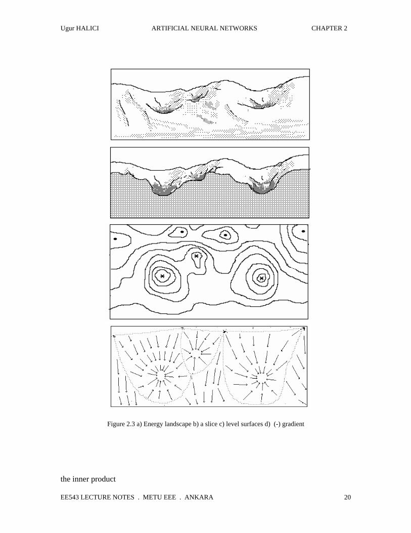
is called the gradient of the function E and extends in the direction of the greatest rate of

change of E and has that rate of change for its length.

If we set E(x)=c, we obtain a family of surfaces known as level surfaces of E, as x takes

on different values. Due to the assumption that E is single valued at each point, one and

only one level surface passes through any given point P [Wylie and Barret 85]. The

gradient of E(x) at any point P is perpendicular to the level surface of E, which passes

through that point. (Figure 2.3)

For a vector field

F(x)=[F F FN1 2( ) ( ) ... ( )x x x ]T (2.4.3)



20

Figure 2.3 a) Energy landscape b) a slice c) level surfaces d) (-) gradient

the inner product



21

∇.F= ∂∂

∂∂

∂∂

Fx

Fx

Fx

N

N

1

1

2

2+ + +.. . (2.4.4)

is called the divergence of F, and it has a scalar value.

Consider a region of volume V and surface S in the phase space of an autonomous

system, and assume a flow of points from this region. From our earlier discussion, we

recognize that the velocity vector dx/dt is equal to the vector field F(x). Provided that the

vector field F(x) within the volume V is "well behaved", we may apply the divergence

theorem from the vector calculus [Wylie and Barret 85, Haykin 94]. Let n denote a unit

vector normal to the surface at dS pointing outward from the enclosed volume. Then,

according to the divergence theorem, the relation

dVdSVS

))(.()).(( xFnxF ∇=∫∫ (2.4.5)

holds between the volume integral of the divergence of F(x) and the surface integral of

the outwardly directed normal component of F(x). The quantity on the left-hand side of

Eq. (2.4.5) is recognized as the net flux flowing out of the region surrounded by the

closed surface S. If the quantity is zero, the system is conservative; if it is negative, the

system is dissipative. In the light of Eq. (2.4.5), we may state equivalently that if the

divergence

∇⋅ =F x( ) 0 (2.4.6)

then the system is conservative and if

∇⋅ <F x( ) 0 (2.4.7)

the system is dissipative, which implies the stability of the system [Haykin 94].



22

2.5. Equilibrium States

A constant vector x* satisfying the condition

F x 0( *) = , (2.5.1)

is called an equilibrium state (stationary state or fixed point) of the dynamical system

defined by Eq. (2.1.2). Since it results in

N1iforxdt

dxi ..0*

== , (2.5.2)

the constant function x(t)=x* is a solution of the dynamical system. If the system is

operating at an equilibrium point, then the state vector stays constant, and the trajectory

with an initial state x(0)=x* degenerates to a single point.

We are frequently interested in the behavior of the system around the equilibrium points,

and try to investigate if the trajectories around the equilibrium points are converging to

the equilibrium point, diverging from it or staying in an orbit around the point or

combination of these.

The use of a linear approximation of the nonlinear function F(x) makes it easier to

understand the behavior of the system around the equilibrium points. Let x=x*+∆x be a

point around x*. If the nonlinear function F(x) is smooth and if the disturbance ∆x is

small enough then it can be approximated by the first two terms of its Taylor expansion

around x* as:

F x x F x F x x( * ) ( *) ( *)+ ≅ + ′∆ ∆ (2.5.3)



23

where

F xx

Fx x

' ( *)*

==

∂∂

(2.5.4)

that is, in particular:

′ ==

FF

xijj

i( *)

( )

*x

x

x x

∂

∂. (2.5.5)

Notice that F(x*) and F '(x*) in Eq. (2.5.3) are constant, therefore it is a linear equation

in terms of ∆x.

Furthermore, since an equilibrium point satisfies Eq. (2.5.1), we obtain

F x x F x x( * ) ( *)+ ≅ ′∆ ∆ (2.5.6)

On the other hand, since

ddt

ddt

( * )x x x+ =∆ ∆ (2.5.7)

the Eq. (2.1.2) becomes

ddt∆ ∆x F x x= ′( *) (2.5.8)

Since Eq. (2.5.8) defines a homogenous differential equation with constant real

coefficient, the eigenvalues of the matrix F '(x*) determines the behavior of the system.



24

Exercise: Give the general form of the solution of the system defined by Eq. (2.5.8)

Notice that, in order to have ∆x(t) to diminish as t→∞, we need the real parts of all the

eigenvalues to be negative.

2.6. Stability

An equilibrium state x* of an autonomous nonlinear dynamical system is called stable, if

for any given positive ε, there exists a positive δ satisfying,

||x(0)-x*|| < δ ⇒ ||x(t)-x*|| < ε for all t >0. (2.6.1)

If x* is a stable equilibrium point, it means that any trajectory described by the state

vector x(t) of the system can be made to stay within a small neighborhood of the

equilibrium state x* by choosing an initial state x(0) close enough to x*.

An equilibrium point x* is said to be asymptotically stable if it is also convergent, where

convergence requires the existence of a positive δ such that

||x(0)-x*|| < δ ⇒ =→∞lim ( ) *t tx x . (2.6.2)

If the equilibrium point is convergent, the trajectory can be made approaching to x* as t

goes to infinity, by choosing again an initial state x(0) close enough to x*. Notice that

asymptotically stable states correspond to attractors of the system.

For an autonomous nonlinear dynamical system the asymptotic stability of an equilibrium

state x* can be decided by the existence of energy functions. Such energy functions are

called also as Liapunov functions since they are discovered by Alexander Liapunov in

the early 1900s to prove the stability of differential equations.



25

A continuous function L(x) with a continuous time derivative L'(x)=dL(x)/dt is a definite

Liapunov function if it satisfies:

a) L(x) is bounded

b) L'(x) is negative definite, that is:

L'(x)<0 for x≠x* (2.6.3)

and

L'(x)=0 for x=x* (2.6.4)

If the condition (2.6.3) is in the form

*for0)(L' xxx ≠≤ (2.6.5)

the Liapunov function is called semidefinite.

Having defined the Liapunov function, the stability of an equilibrium point can be

decided by using the following theorem:

Liapunov's Theorem: The equilibrium state x* is stable (asymptotically stable), if there

exists a semidefinite (definite) Liapunov function in a small neighborhood of x*.

The use of Liapunov functions makes it possible to decide the stability of equilibrium

points without solving the state-space equation of the system. Unfortunately there is not

any formal way to find a Liapunov function, mostly it is determined in a trial and error

fashion. If we are able to find a Liapunov function, then we state the stability of the

system. However, the inability to find a Liapunov function, does not imply the instability

of the system.



26

Often convergence of neural networks is guaranteed by introducing an energy function

together with the network itself. In fact the energy functions are Liapunov functions, so

they are non-increasing along trajectories. Therefore the dynamics of the network can be

visualized in terms of some multidimensional 'energy landscapes' as given previously in

Figure 2.3. The attractors of the dynamical system are the local minima of the energy

function surrounded with 'valleys' corresponding to the basins of attraction (Figure 2.4).

Figure 2.4. Energy landscape and basin attractions

2.7. Effect of input and initial state on the attraction

The convergence of a network to an attractor of the activation dynamics may be viewed

as a retrieval process in which the fixed point is interpreted as the output of the neural

network. As an example consider the following network dynamic:

)()()( ij

jjiiii xwftxtxdtd θ++−= ∑ (2.7.1)



27

Assume that the weight matrix W is fixed and the network is specified through θ and

initial state x(0). Both θ and x(0) are ways of introducing an input pattern into the

network, although they play distinct dynamical roles [Bressloff and Weir 91].

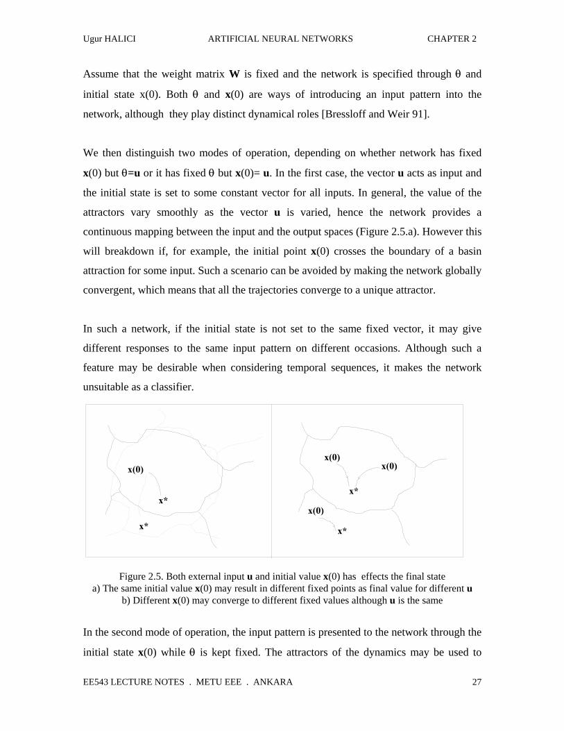
We then distinguish two modes of operation, depending on whether network has fixed

x(0) but θ=u or it has fixed θ but x(0)= u. In the first case, the vector u acts as input and

the initial state is set to some constant vector for all inputs. In general, the value of the

attractors vary smoothly as the vector u is varied, hence the network provides a

continuous mapping between the input and the output spaces (Figure 2.5.a). However this

will breakdown if, for example, the initial point x(0) crosses the boundary of a basin

attraction for some input. Such a scenario can be avoided by making the network globally

convergent, which means that all the trajectories converge to a unique attractor.

In such a network, if the initial state is not set to the same fixed vector, it may give

different responses to the same input pattern on different occasions. Although such a

feature may be desirable when considering temporal sequences, it makes the network

unsuitable as a classifier.

Figure 2.5. Both external input u and initial value x(0) has effects the final state

a) The same initial value x(0) may result in different fixed points as final value for different u b) Different x(0) may converge to different fixed values although u is the same

In the second mode of operation, the input pattern is presented to the network through the

initial state x(0) while θ is kept fixed. The attractors of the dynamics may be used to



28

represent items in a memory while the initial states are the stimulus to remember the

stored memory items. The initial states that contain incomplete or erronous information

may be considered as queries to the memory. The network then converges to the

complete memory items that best fits the stimulus (Figure 2.5.b). Thus in contrast to the

first mode of operation, which ideally uses a globally convergent network, this form of

operation exploits the fact that there are many basins of attraction to act as a content

addressable memory. However, as a result of inappropriate choices for the weights, there

may be a complication arising from the fixed points of the network where the memory

items are indented to reside. Although the intention is to have fixed points corresponding

only to the stored memory items, it may appear undesired fixed points called spurious

states [Bresloff and Weir 91].

2.8 Cohen-Grossberg Theorem

The idea of using energy functions to analyze the behavior neural networks was

introduced during the first half of the 1970s independently in [Amari 72], [Grossberg

72] and [Little 74]. A general principle, known as Cohen-Grossberg theorem is based on

the Grossberg's studies during the previous decade. As described in [Cohen and

Grossberg 83] it is used to decide the stability of a certain class of neural networks.

Theorem: Consider a neural network with N processing elements having output signals

fi(ai) and transfer functions of the form

ddt

a a a w f a i Ni i i i i ji j jj

n= − =

=∑α β( )( ( ) ( )) ..

11 (2.8.1)

satisfying constraints:

1) Matrix W=[wij] is symmetric, that is wij=wji, and all wij>0

2) Function αi(a) is continuous and α i a for a( ) > >0 0



29

3) Function fj(a) is differentiable and 00))(()( ≥≥=′ aforafdadaf jj

4) (βi(ai)-wii)<0 as ai →∞

5) Function βi(a) is continuous for a>0

6) Either ∞=+→

)(lim0

aia

β or ∞=∞< ∫+→ds

sbuta

i

a

ia )(

1)(lim00 α

β for some a >0.

If the network's state a(0) at time 0 is in the positive orthant of Rn (that is ai(0)>0

i=1..N), then the network will almost certainly converge to some stable point also in the

positive orthant. Further, there will be at most a countable number of such stable points.

Here the statement that the network will "almost certainly" converge to a stable point

means that this will happen except for certain rare choices of the weight matrix. That is,

if weight matrix W is chosen at random among all possible W choices, then it is virtually

certain that a bad one will never be chosen.

In Eq. (2.8.1), which is describing the dynamic behavior of the system, αi(ai) is the

control parameter for the convergence rate. The decay function βi(ai) allows us to place

the system's stable attractors in appropriate positions of the state space.

In order to prove the part related to the stability of the system, the theorem uses Liapunov

function approach by showing that, under the given conditions, the function

dssfsafafwE i

aN

ijji

N

iiji

N

j

i

)()()()(011 1

21 ′−+= ∑∫∑∑

== =

β (2.8.2)

is an energy function of the system. That is, E has negative time derivative on every

possible trajectory that the network's state can follow.

By using the condition (1), that is W is symmetric, the time derivative of the energy

function can be written as



30

2

11

)()()()( ⎥⎦

⎤⎢⎣

⎡−′−= ∑∑

==jj

N

jjiiii

N

iiii afwaafa

dtdE βα (2.8.3)

and it has negative value for a≠ a* whenever conditions (2) and (3) are satisfied.

The condition (4) guarantees that any a* to has a finite value, preventing them to

approach infinity.

The rest of the conditions (the condition wij>0 in (1) and the conditions (5) and (6)) are

requirements to prove that the solution always stays in the positive orthant and satisfies

some other detailed mathematical requirements, which are not so easy to show, requires

some sophisticated mathematics.

While the converge to a stable point in the positive orthant is important for a model

resembling a biological neuron, we do not care such a condition for artificial neurons as

long as they converge to some stable point having finite value. Whenever the function f

is a bounded, that is |f(a)|<c for some positive constant c, any state can not take infinite

value. However for the stability of the system still remain the constraints:

a) Symmetry:

w w i j 1 Nji ij= =, .. (2.8.4)

b) Nonnegativity:

Niai ..10)( =≥α (2.8.5)



31

c) Monotonocity:

00))(()( ≥≥=′ aforafdadaf (2.8.6)

This form of Cohen-Grossberg theorem states that if the system of nonlinear equations

satisfies the conditions on symmetry, nonnegativity and monotonocity, then the energy

function defined by Eq. (2.8.1) is a Liapunov function of the system satisfying

*0 ii aafordtdE

≠< (2.8.7)

and the global system is therefore asymptotically stable [Haykin 94].

2.9 Hopfield Network

The continuous deterministic Hopfield model which is based on continuous variables

and responses, is proposed in [Hopfield 84] to extend their discrete model of the

processing elements [Hopfield 82] to resemble actual neurons more closely. In this

extended model, the neurons are modeled as amplifiers in conjunction with feedback

circuits made up of wires, resistors and capacitors which suggests the possibility of

building these circuits using VLSI technology. The circuit diagram of the continuous

hopfield network is given in Figure 2.6. This circuit has a nerobiological ground as

explained below:



32

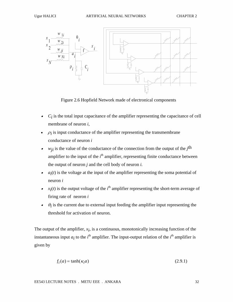
Figure 2.6 Hopfield Network made of electronical components

• Ci is the total input capacitance of the amplifier representing the capacitance of cell

membrane of neuron i,

• ρi is input conductance of the amplifier representing the transmembrane

conductance of neuron i

• wji is the value of the conductance of the connection from the output of the jth

amplifier to the input of the ith amplifier, representing finite conductance between

the output of neuron j and the cell body of neuron i.

• ai(t) is the voltage at the input of the amplifier representing the soma potential of

neuron i

• xi(t) is the output voltage of the ith amplifier representing the short-term average of

firing rate of neoron i

• θi is the current due to external input feeding the amplifier input representing the

threshold for activation of neuron.

The output of the amplifier, xi, is a continuous, monotonically increasing function of the

instantaneous input ai to the ith amplifier. The input-output relation of the ith amplifier is

given by

f a ai i( ) tanh( )= κ (2.9.1)



33

where κi is constant called the gain parameter.

Notice that, since

tanh( )x e ee e

x x

x x=−

+

−

− (2.9.2)

the amplifier transfer function is in fact a sigmoid function

f a ee e

ia

a a

i

i i( ) = −

+=

+−

−

− −11

21

12

κ

κ κ (2.9.3)

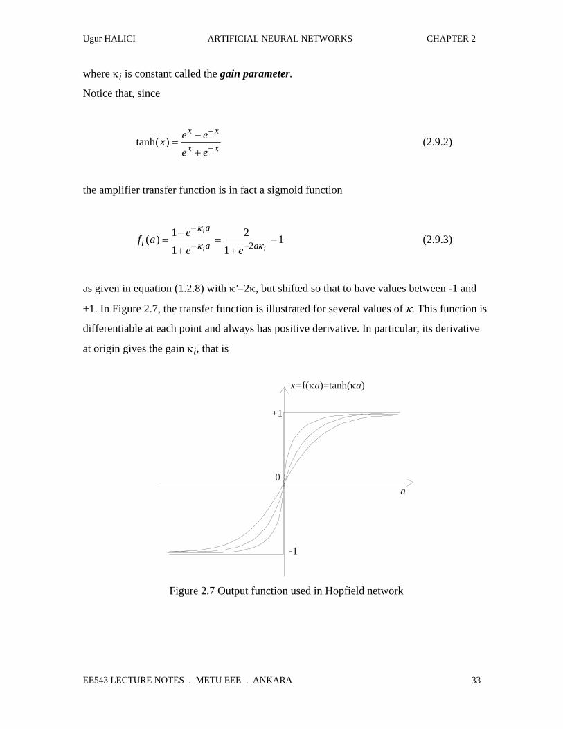
as given in equation (1.2.8) with κ'=2κ, but shifted so that to have values between -1 and

+1. In Figure 2.7, the transfer function is illustrated for several values of κ. This function is

differentiable at each point and always has positive derivative. In particular, its derivative

at origin gives the gain κi, that is

x= a af( )=tanh( )κ κ

0

+1

-1

a

Figure 2.7 Output function used in Hopfield network



34

κii

adfda

= =0 (2.9.4)

The amplifiers in the Hopfield circuit correspond to the neurons. A set of nonlinear

differential equations describes the dynamics of the network. The input voltage ai of the

amplifier i is determined by the equation

Cii

R i ji j jj

ida t

dta t w f a t

i

( ) ( ) ( ( ))= − + +∑1 θ (2.9.5)

while the output voltage is

)( iii afx = (2.9.6)

In Eq. (2.9.5) Ri is determined as 1/Ri= ρi+Σj wji

The state of the network is described by an N dimensional state vector where N is the

number of neurons in the network. The ith component of the state vector is given by the

output value of the ith amplifier taking real values between -1 and 1. The state of the

network moves in the state space in a direction determined by the above nonlinear dynamic

equation (2.9.5).

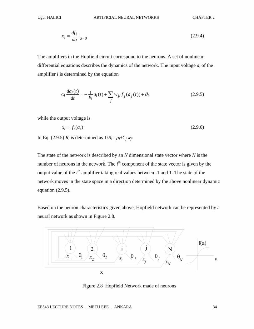
Based on the neuron characteristics given above, Hopfield network can be represented by a

neural network as shown in Figure 2.8.

Figure 2.8 Hopfield Network made of neurons



35

The energy function for the continuous Hopfield model is given by the formula

∑∫∑∑∑ −+−= −

iiii

ii

jjji

ixdxxfxxwE

ix

iRθ)(1

0

121 (2.9.7)

where fi-1 is the inverse of the function fi, that is

f x ai i i− =1( ) (2.9.8)

In particular, for the transfer function defined by the equation (2.9.3), we have

f x xxi

− = −−+

1 11

( ) ln (2.9.9)

which is shown in Figure 2.9.

Figure 2.9 Inverse of the output function



36

Exercise: What happens to the system's energy if sigmoid function is used instead of tanh

function.

In [Hopfield 84], it is shown that the energy function given in equation 2.9.7 is an

appropriate Lyapunov function for the system ensuring that the system eventually reaches a

stable configuration if the network has symmetric connections, that is wij=wji. Such a

network always converges to a stable equilibrium state, where the outputs of the units

remain constant.

For energy E of the Hopfield network to be a Lyapunov function, it should satisfy the

following constraints:

a) E(x) is bounded

b) dEdt

≤ 0

Because the function tanh(κa) is used in the system as the output function, it limits the state

variable to take value between -1<xi<1. Furthermore, because the integral of the inverse of

this function is bounded if -1<xi<1, the energy function given by Eq. (2.9.7) is bounded.

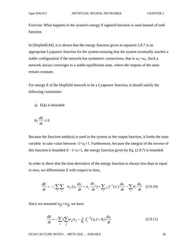
In order to show that the time derivative of the energy function is always less than or equal

to zero, we differentiate E with respect to time,

∑∑∑∑ −++−= −

i

ii

iii

i

jj

i

iiji

j dtdx

dtdx

xfdt

dxx

dtdx

xwdtdE

iRθ)()( 11

21 (2.9.10)

Since we assumed wji=wij, we have

dEdt

w x f x dxdtj

ji ji

R i i ii

i= − − +∑∑ −( ( ) )1 1 θ (2.9.11)



37

By the use of equations (2.9.6) and (2.9.8) in (2.9.5), we obtain

w x f x dadtji j

jR i i i Ci

ii

∑ − + =−1 1( ) θ . (2.9.12)

Therefore Eq. (2.9.11) results in

dEdt

C dadt

dxdti

i

i i= −∑ (2.9.13)

On the other hand notice that, by the use of Eq. (2.9.8) we have

dadt

ddx

f x dxdt

ii

i= −1( ) (2.9.14)

so

dEdt

Cdf x

dxdxdti

i

i i= −∑−1

2( )( ) (2.9.15)

Due to equation (2.9.9) we have

df x

dxi−

≥1

0( )

(2.9.16)

for any value of x. So Eq. (2.9.15) implies that,

dEdt

≤ 0 (2.9.17)



38

Therefore the energy function described by equation (2.9.7) is a Lyapunov function for the

Hopfield network when the connection weights are symmetrical. This means that, whatever

the initial state of the network is, it will converge to one of the equilibrium states depending

on the basin attraction in which the initial state lies.

Another way to show that the Hopfield network is stable is to apply the Cohen-Grossberg

theorem given in section 2.8. For this purpose we reorganize the Eq. (2.9.5) as:

da tdt

a t w f a tiCi R i i ji j j

ji

( ) (( ( ) ) ( ) ( ( )))= − + − −∑1 1 θ (2.9.18)

If we compare Eq. (2.9.18) with Eq. (2.8.1) we recognize that in fact Hopfield network is a

special case of the system defined in Cohen-Grossberg theorem:

αi iaCi

( ) ↔ 1 (2.9.19)

and

β θ( ( )) ( )a t a tRii

ii↔ − + (2.9.20)

and

wij ↔ -wij (2.9.21)

satisfying the conditions on

a) symmetry, because wij=wij implies

-wij=-wji (2.9.22)

b) nonnegativity, because



39

αi iaCi

( ) = 1≥0 (2.9.23)

c) monotonocity, because

0)tanh()(' ≥= adtdaf ii κ (2.9.24)

Therefore, according to the Cohen-Grossberg theorem, the energy function defined as

daafaafafwE iii

jjiiiji j

iR

ia

)()()()()( 1

021 ′+−−−= ∫∑∑∑ θ (2.9.25)

is a Lyapunov function of the Hopfield network and the network is globally asymptotically

stable.

In fact, the energy equation defined by equation (2.2.25) may be organized as

daaf

daafaafafwE

ia

ia

iR

ii

ijiij

i j

)(

)()()(

0

0

121

′−

′+−=

∫∑

∫∑∑∑

θ (2.9.26)

Notice that

)()0()()(0 ii

aaffafdaafi =−=′∫ (2.9.27)

and also

dxxfafdadaafa iii xaf

f

a)())(()( 1

0

)(

)0(0

−∫∫∫ ==′ (2.9.28)

Therefore the energy equation defined by Eq. (2.9.25) becomes



40

iiii

jiiji j

xdxxfxxwEix

iR θ∑∫∑∑∑ −+−= − )(1

0

121 (2.9.29)

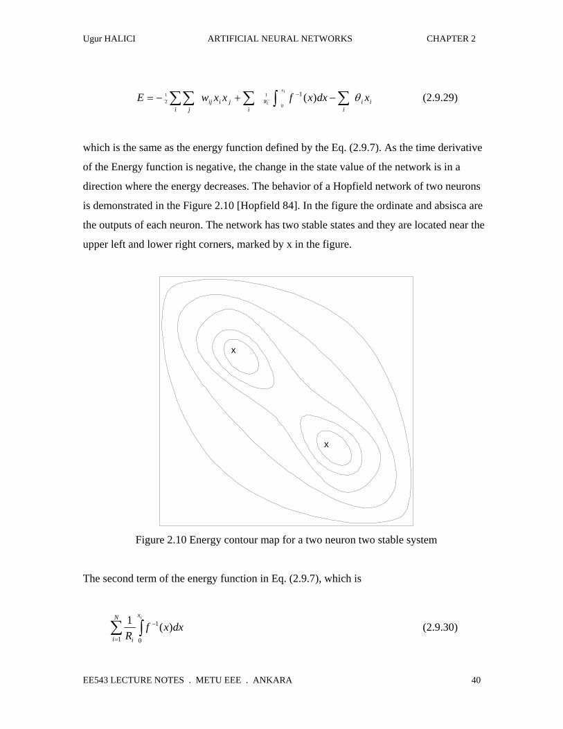
which is the same as the energy function defined by the Eq. (2.9.7). As the time derivative

of the Energy function is negative, the change in the state value of the network is in a

direction where the energy decreases. The behavior of a Hopfield network of two neurons

is demonstrated in the Figure 2.10 [Hopfield 84]. In the figure the ordinate and absisca are

the outputs of each neuron. The network has two stable states and they are located near the

upper left and lower right corners, marked by x in the figure.

Figure 2.10 Energy contour map for a two neuron two stable system

The second term of the energy function in Eq. (2.9.7), which is

∑ ∫=

−N

i

x

i

i

dxxfR1 0

1 )(1 (2.9.30)

x

x



41

alters the energy landscape. The value of the gain parameter determines how close the

stable points come to the hypercube corners. In the limit of very high gain, κ→∞, this term

approaches to zero and the stable points of the system lie just at the corners of the

Hamming hypercupe where the value of each state component is either -1 or 1. For finite

gain, the stable points move towards the interior of the hypercube. As the gain becomes

smaller these stable points gets closer. When κ=0, only a single stable point exists for the

system. Therefore the choice of the gain parameter is quite important for the success of the

operation [Freeman 91].



42

2.10. Discrete time representation of recurrent networks

Consider the dynamical system defined by the Eq. (2.1.2). The change ∆x(t) in the value of

x(t) in a small amount of time ∆t can be approximated as:

ttt ∆≅∆ ))(())(( xFx (2.10.1)

Hence the value of x(t+∆t) in terms of this amount of change,

x(t+∆t)=x(t)+ ∆(x(t)) (2.10.2)

becomes

x(t+∆t)=x(t)+F(x(t))∆t. (2.10.3)

Therefore, if we start with t=0 and observe the output value at each time elapse of ∆t, then

the value of x (t) at kth observation may be expressed by using the value of the previous

observation as

x(k)=x(k-1)+F(x(k-1))∆t k=1,2 ... (2.10.4)

or equivalently,

x(k)=x(k-1)+ηF(x(k-1)) k=1,2 ... (2.10.5)

where η is used instead of ∆t to represent the approximation step size and it should be

assigned a small value for a good approximation. However, depending on the properties of

the function F, the system may also be represented by other discrete time equations.



43

For example, for the continuous time continuous state Hopfield network described in by

Equation (2.9.5) we may use the following discrete time approximation:

x(k)=x(k-1)+ η [-x(k-1)+tanh(κ(WTx(k-1)+θ))], k=1,2 ... (2.10.6)

However in Section 4.3 we will examine a special case of the Hopfield network where the

state variables are forced to take discrete values in binary state space. So the discrete time

dynamical system representation given by Eq. 2.10.6 will further be modified, by using

sign(WTx(k-1)+θ) where sign is a special case of the sigmoid function in which the gain is

infinity.

We have observed that the stability of continuous time dynamical systems described by Eq.

2.1.1 are implied by the existence of a bounded energy function with a time derivative that

is always less or equal to zero. The states of the network resulting in zero derivatives are

the equilibrium states.

Analogously, for a discrete time neural network with an excitation

x(k)=x(k-1)+G(x(k-1)) k=1,2 ... (2.10.7)

the stability of the system is implied by the existence of a bounded energy function so that

the difference in the value of the energy should always be negative as the system changes

states.

When G(x)=ηF(x) the stable states of the continuous and discrete time systems described

by equations 2.1.1 and 2.10.7 respectively are almost the same for small values of η.

However if η is not small enough, some stable states of the continuous system may

becomes unreachable in discrete time.

CHAPTER II Recurrent Neural...

Documents

Transcript of CHAPTER II Recurrent Neural...