21

CHAPTER FOUR

Results and discussion:

The heat equation is an parabolic partial differential equation that

describes of the distribution of heat (or variation in temperature) in a

given region over time. In this chapter we have discussed finite difference

method such as (Schmidt method, Crank-Nicolson method, Iterative

method, and Du Fort Frankle method) for one dimensional heat

equation and, (ADE) method for two dimensional heat equation.

The equation (4.1) is given below, for one dimensional heat equation

(4.1)

Where ⁄ is the diffusivity of the substance ( ⁄ )

= constants

x = distance

t = temperature

k = coefficient of conductivity

= density of material

s = specific heat

22

(1). Schmidt method: (explicit formula).

Conceders a rectangular mesh in the x-t plane with spacing along

direction and along time t direction. Denoting a mesh point ( )

( ) as simply we have,

And

Substituting these in (4.1), we obtain

=

[ ]

Or = ( ) (4.2)

Where ⁄ This formula enable us

to determine the value of u at the ( ) mesh point in terms of the

known function values at the point and at the instant it is a

relation between the function values at the time levels and and is

therefore called a 2-level formula in schematic form (4.2) is shown in

fig. (4.1).

23

( ) ( ) level

level

( ) ( ) ( )

Hence (4.2) is called the Schmidt explicit formula which is valid only for

0 <

.

Remark. In particular when

equation (4.2) reduces to

( ) ( )

Which shows that the value of at at time is the mean of the

-value at and at time . This known as bender-Schmidt

recurrence relation, gives the values of at the internal mesh points with

the help of boundary condition.

Example: 1

Use bender –Schmidt formula to solve the heat equation

With the conditions ( ) ( ) ( )

Setting we see that when

Solution:

The initial values are ( ) ( )

Fig. (4.1).

24

( ) ( ) ( )

Further, ( ) ( )

For bender -Schmidt formula gives

( )

( )

( )

Similarly for , we obtain

( )

( )

( )

(2). The crank- Nicholson method

We have seen that the Schmidt scheme is computationally simple and for

convergent results

⁄ To obtain more accurate

results, should be small i.e. is necessarily very small. This makes the

computations exceptionally lengthy as more time-levels would be

required to cover the region. A method that does not restrict and also

reduces the volume of calculation was proposed by Crank and Nicolson

in 1947. According to this methods, ⁄ is replaced by the average

of its central-difference approximations on the and ( ) time

rows. Thus (4.1) is reduced to.

25

{

}

{

}

Or ( )

( ) ( )

Where ⁄

Clearly the left side of (4.4) contains three unknown values of u at the

( ) level while all the three values on the right are known values

at the level. Thus (4.4) is a 2-level implicit relation and is known as

Crank–Nicolson formula. It is convergent for all finite values of It is

computational model is given in Fig. (4.2).

( ) ( ) ( ) ( ) level

level

( ) ( ) (i+1, j)

The crank-Nicholson grid. Fig (4.2).

If there are n internal mesh points on each row, then the relation (4.4)

gives n simultaneous equations for the n unknown values in terms of the

unknown boundary values. These equations can be solved to obtain the

26

i

values at these mesh points. Similarly, the values at the interval mesh

points at all rows can be found. A method such as this in which the

calculation, of a known mesh value necessitates the solution of a set of

simultaneous equation, is known as an implicit scheme.

Example: 2

Solve the equation

by crank-Nicholson

method.

Given that ( ) ( ) ( )

Solution:

By Giving and , taking

, we get .

j 0 1 2 3 4 5

0 0 20 20 20 20 100

1 0 100

Then crank-Nicolson formula becomes

= 0+20+0+ i.e ( )

= 20+20+ + i.e ( )

= 20+20+ + i.e ( )

= 20+100+ +100 i.e ( )

Now ( ) ( ) gives =180 ( )

4( ) ( ) give ( )

Then15( ) – 4( ) gives 209 ie

Table (4.1)

27

From( ) we get i.e = 30.75

From ( ) we get i.e = 10.05

From ( ) we get

i.e = 62.69

Thus the required values are 10.05, 20.2, 30.75 and 62.68.

(3). Iterative method for an explicit scheme

The iterative methods can be applied to solve the finite-difference

equations can be obtained in the preceding section. In the Crank-Nicolson

method we have

( ) ( )

(4.4)

A B C

0

D E F

( ) [ ] ( )

= [ ]

Fig(4.3).

28

[ ] [ ]

[ ]

[ ]

Or an Implicit scheme from (3.4) we have

(1+ ) =

( + ) + +

( 2 + )

(4.5)

Here only , and are unknown while all others are

known since these were already computed in the th step

Denote: = +

( + ) (4.6)

And dropping (4.6) becomes =

( ) ( + ) +

This gives the iteration formula

=

( ){

( ) ( )} +

(4.7)

Which expresses the ( ) iterates in terms of the iterates only.

This is known as the Jacobi iteration formula,

As the latest value of i.e. ( ) is already available the

convergence of the iteration formula (4.7) can be improved by replacing

by

A accordingly (4.7) may be written as

=

( ){

( ) ( )} +

(4.8)

This is known as Gauss-Seidal iteration formula

29

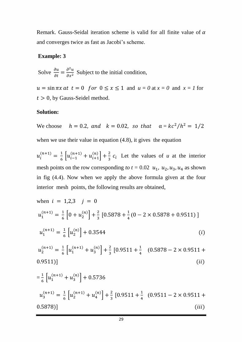
Remark. Gauss-Seidal iteration scheme is valid for all finite value of

and converges twice as fast as Jacobi’s scheme.

Example: 3

Solve

Subject to the initial condition,

and u = 0 at x = 0 and x = 1 for

, by Gauss-Seidel method.

Solution:

We choose = ⁄ ⁄

when we use their value in equation (4.8), it gives the equation

( )

[

( )

( )]

Let the values of u at the interior

mesh points on the row corresponding to t = 0.02 as shown

in fig (4.4). Now when we apply the above formula given at the four

interior mesh points, the following results are obtained,

when

( )

[

( )]

( )

( )

[

( )] ( )

( )

[

( )

( )]

(

) ( )

=

[

( )

( )]

( )

[

( )

( )]

(

) ( )

30

( )

[

( ) ]

( )

=

[

( )] ( )

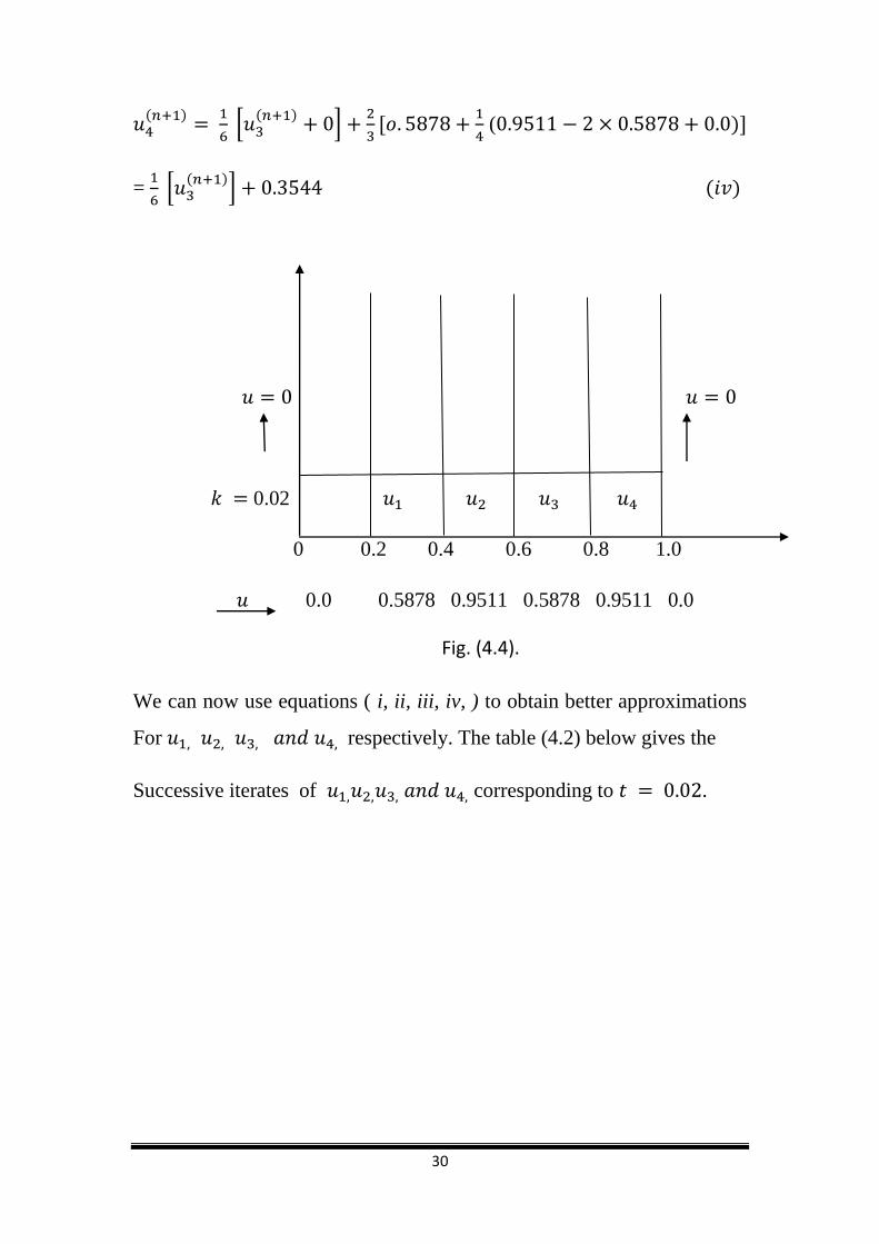
0.02

0 0.2 0.4 0.6 0.8 1.0

0.0 0.5878 0.9511 0.5878 0.9511 0.0

We can now use equations ( i, ii, iii, iv, ) to obtain better approximations

For respectively. The table (4.2) below gives the

Successive iterates of corresponding to .

Fig. (4.4).

31

(4). Du fort and Frankel method:

If we replace the derivatives in (4.1) by the central difference

approximations,

and

We obtain =

[ ]

i.e. = +2 [ ] (4.8)

Where ⁄ this difference equation is called the Richardson

Scheme which is a 3-level method.

0.0 0.2 0.4 0.6 0.8 1.0

u=(x) 0.0 0.5878 0.9511 0.9511 0.5878 0.0

n=0 0.0 0.5878 0.9511 0.9511 0.5878 0.0

n=1 0.0 0.5129 0.8176 0.8078 0.4890 0.0

n=2 0.0 0.4907 0.7900 0.7868 0.4855 0.0

n=3 0.0 o.4861 0.7858 0.7855 0.4853 0.0

n=4 0.0 0.4854 0.7854 0.7854 0.4853 0.0

n=5 0.0 0.4853 0.7854 0.7854 0.4853 0.0

32

If we replace by the mean of the value and i.e

( + ) in (4.8), then we get

= [ + 2 ( + ) + ]

On simplification it can be written as

=

+

{ } (4.9)

This difference scheme is called Du fort Frankel method which is a

3-level explicit method. Its computational model is given in fig (4.5).

( ) ( )th level

( ) ( ) j th level

( ) ( ) th level

Example: 4

Solve the equation

Fig (4.5).

33

Subject to the conditions ( ) ( )

( ) using the Du fort–Frankel method, carry out. Computations

for two levels, taking

Solution:

Here

Also the initial values are

√

√

and all boundary values are zero.

By Du fort-Frankel formula

[ ]

To start the calculations we need

We may take from Schmidt method

For :

[ ]

[√ ⁄ ]

[ ]

[√ ⁄ ]

Comparative study of different methods

We are solving heat equation by finite difference method and comparing

both results which are obtained by Bender-Schmidt and Crank Nicolson

Methods with analytical solution.

34

Example: 5

Find the analytical solution of the parabolic equation when

( ) ( ) and ( ) ( ) taking , and

,

Find the values up to .

Solution:

It is already given parabolic equation

and also given the boundary condition, ( ) ( )

the initial condition ( ) ( ) we can write parabolic equation

in the form,

(1)

where

Let (2)

where is the function of only and is the function of only.

Differentiating (2) partially , we get

(3)

(4)

Let (3) and (4) equal

Put the values of (

) and (

) in (1) we get,

35

= =

Separating variables, we get

Where

Now,

We have,

, put the value of and in equation (2) we get,

( )

(5)

36

Now, put the value of ( ) , where in equation (5), we get

Let arbitrary constant we have so

( )

(6)

put the value of ( ) , where in equation (6), we get

Put the value of p in equation (6)

(

)

(

)

(

)

(

)

(7)

Where ∑

∑ (

)

(

)

(8)

Now we find the value of by Fourier series,

∫ ( )

(

)

∫ ( )

(

)

37

∫

(

)

∫

(

) (9)

Integration first part from equation (9) by the form of integral,

+……

[ (

)

(

)

(

)

(

) ]

(

)

(10)

Integration second part from equation (9)

[{

(

)

(

)

}

{

(

)

(

)

}

{ (

)

(

) } ]

[

(

)

{

(

) }]

[

(

)

( )]

[

( )] (11)

putting the value of (10) and (11) in (9) we get,

( )

4

4

0

0

4

[

38

( )

When = 0

( )

Put value of in equation (8), we get

(

)

(

)

(12)

Where

√

(

)

√

(

)

(

)

(

)

.

Analytical solution for

Now we solve (Example: 5) by numerical methods

39

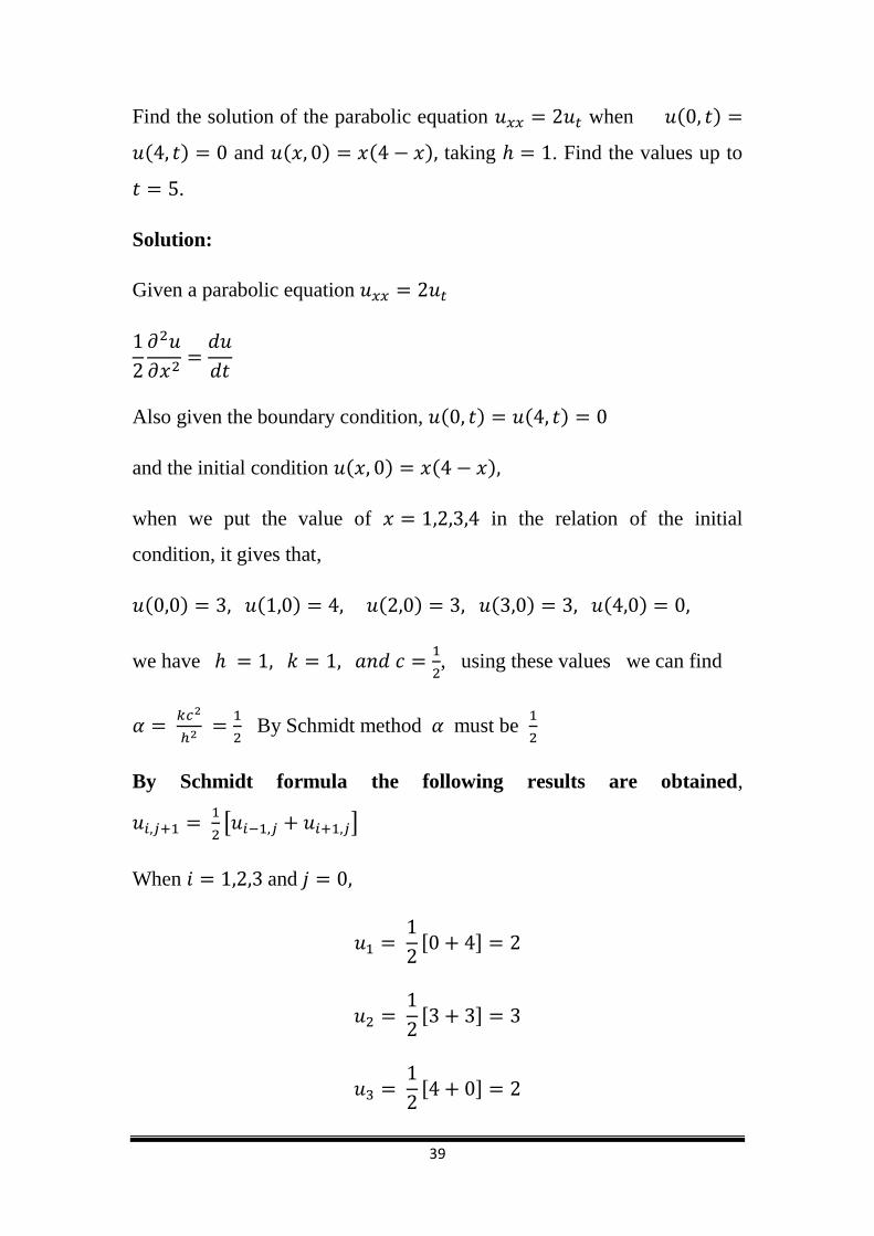
Find the solution of the parabolic equation when ( )

( ) and ( ) ( ) taking . Find the values up to

.

Solution:

Given a parabolic equation

Also given the boundary condition, ( ) ( )

and the initial condition ( ) ( )

when we put the value of in the relation of the initial

condition, it gives that,

( ) ( ) ( ) ( ) ( )

we have

, using these values we can find

By Schmidt method must be

By Schmidt formula the following results are obtained,

[ ]

When and

40

When

When

Now solve by Crank-Nicolson formula:

( )

( )

Put

When

( )

( )

( )

41

When the initial conditions are given in ( ) ( ) ( ) we get.

( )

( )

( )

When we solve the equations ( ) ( ) ( ) by manual or by calculator it

gives that,

,

When

In the same way can we find

,

Result: First step using the Analytical solution and Crank-Nicolson,

Bender-Schmidt,

Analytical result

2.1356 3.032585 2.1356

Schmidt 2 3 2

Crank 2.176470588 3.0588233529 2.176470588

Second step using the Crank-Nicolson and Bender-Schmidt

Schmidt 1.5 2 1.5

Crank 1.615916955 2.283737023 1.615916955

42

Discussion:

The results obtained by analytical methods are always providing accurate

solution but numerical solution always providing approximate result. But

among these numerical methods Crank-Nicolson method was providing

fast convergence in comparison to Bender-Schmidt method. Since it is

not possible to solve every partial differential equation analytically so

numerical methods providing a good agreement in those cases where

solutions not exist or we are unable to solve partial differential equation

analytically.

Example: 6

Solve the heat equation

subject to the condition

( ) ( )

⁄

( )

( ) ⁄

Take

and according to Bandre-Schmidt equation.

Solution:

Using Bandre-Schmidt formula

from Bandre-Schmidt equation.

and

now we find

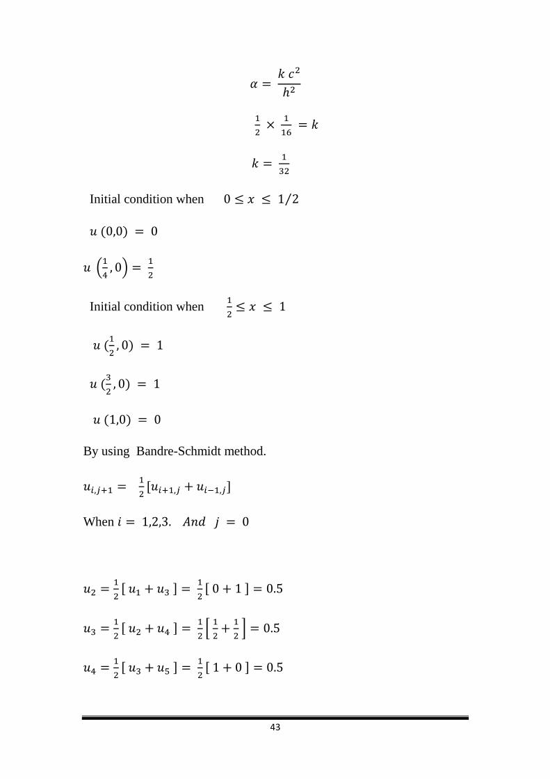
43

Initial condition when ⁄

( )

(

)

Initial condition when

(

)

(

)

( )

By using Bandre-Schmidt method.

When

[

]

44

When

When

Boundary t boundary condition

0 u12 u13 u14 0

0 u7 u8 u9 0

0 u2 u3 u4 0

0 1\2 1 1 0

0 1\4 1\2 3\4 1 x

Fig (4.8)

45

Table of the value:

j i 0 1 2 3 4

0 0 0.5 1 0.5 0

1 0 0.5 0.5 0.5 0

2 0 0.25 0.25 0.25 0

3 0 0.25 0.25 0.25 0

Fig (4.9)

Now, solve by crank-Nicolson method:

Crank-Formula is given below,

( ) (

)

When

and the formula will be

The initial conditions are ( ) , (

)

(

) ,

(

) ( )

When

46

3

When we solve the equations we get,

When

When solving these equations we get,

,

Now, the results which are obtained by Bender-Schmidt and Crank

Nicolson methods are given below,

The results obtained by Crank-Nicolson and Schmidt methods are given

in the following table.

47

At first level.

Schmidt 0.5 0.5 0.5

Crank 0.44117647 0.6470588 0.44117647

The results at second level.

Schmidt 0.25 0.5 0.25

Crank 0.207035455 0.35985967 0.422710

Discussion:

Since Bender Schmidt is work only for ⁄ but crank-Nicolson

work properly for any value of and also in the above example we are

solving the given problem by both method to the result between them and

we see the result for Crank better than Schmidt, since Bender-Schmidt

using level value for calculating value at nodal points but Crank-

Nicolson using and level so Crank is better in comprising to

Bender.

Solution of two dimensional heat equation:

(

) ( )

Where ⁄ is the diffusivity of the substance ( ⁄ )

The methods employed for the solution of one dimensional heat equation

can be readily extended to the solution of (4.10). Consider a square region

48

and assume that u is known at all points within and

the boundary of this square

fig. (4.6)

If be the step–size then a mesh point ( ) ( ) may

be denoted as simply( ). By replacing the derivatives in (4.10) by

their finite difference approximation, we get,

49

{( ) (

)}

( )

( )

Where ⁄

This equation needs the five points available on the nth plane.

The computation process consists of point-by point evaluation in the

( ) the plane using the points on the nth plane. It is followed by

plane-By–plane evaluation. This method is known as ADE (Alternating

Direction Explicit) method.

Example: 7

Solve the equation

subject to the initial conditions

( ) and the conditions

( ) on the boundaries, using ADE method with

(calculate the results for one time level).

Solution:

From the equation (4.11) for two dimensions becomes,

( )

( ) ( )

The mesh points and the computational model is given in fig (4.7).

At the zeros level ( ) the initial and boundary condition a

50

fig (4.7).

51

and

Now we calculate the mesh values at the first level:

For ( ) gives

( ) ( )

( ) ( ) we get

( )

(

) +

(

)

(

√

√

√

√

)

( ) in (2)

( )

{(

) (

) }

(√

)

{ (

√

)

( √

)

}

( ) in (2)

( )

52

{ (

) (

)

}

(

)

( ) in (2)

( )

(

)

(

)

(

)

Similarly the mesh values at the second and higher level can be

calculated.