
CHAPTER EIGHT
27
1 CHAPTER EIGHT PORTFOLIO ANALYSIS
-
Upload
mathilda-sean -
Category
Documents
-
view
22 -
download
0
description
CHAPTER EIGHT. PORTFOLIO ANALYSIS. THE EFFICIENT SET THEOREM. THE THEOREM An investor will choose his optimal portfolio from the set of portfolios that offer maximum expected returns for varying levels of risk, and minimum risk for varying levels of returns. THE EFFICIENT SET THEOREM. - PowerPoint PPT Presentation
Transcript of CHAPTER EIGHT

1
CHAPTER EIGHT
PORTFOLIO ANALYSIS
2
THE EFFICIENT SET THEOREM
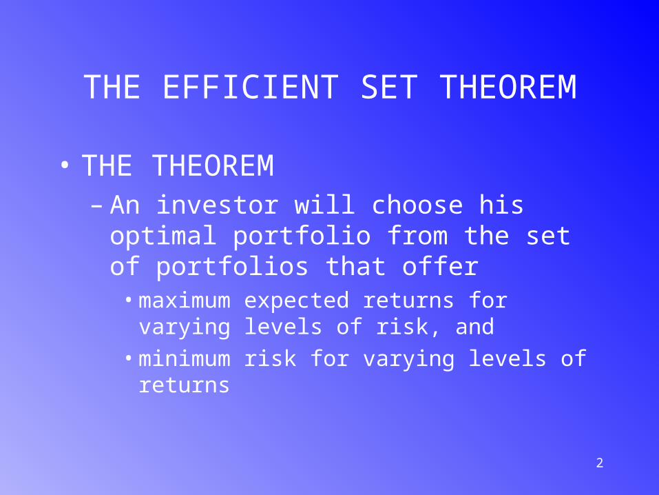
• THE THEOREM– An investor will choose his optimal portfolio
from the set of portfolios that offer• maximum expected returns for varying levels of
risk, and
• minimum risk for varying levels of returns

3
THE EFFICIENT SET THEOREM
• THE FEASIBLE SET– DEFINITION: represents all portfolios that
could be formed from a group of N securities

4
THE EFFICIENT SET THEOREM
THE FEASIBLE SETrP
P0
5
THE EFFICIENT SET THEOREM
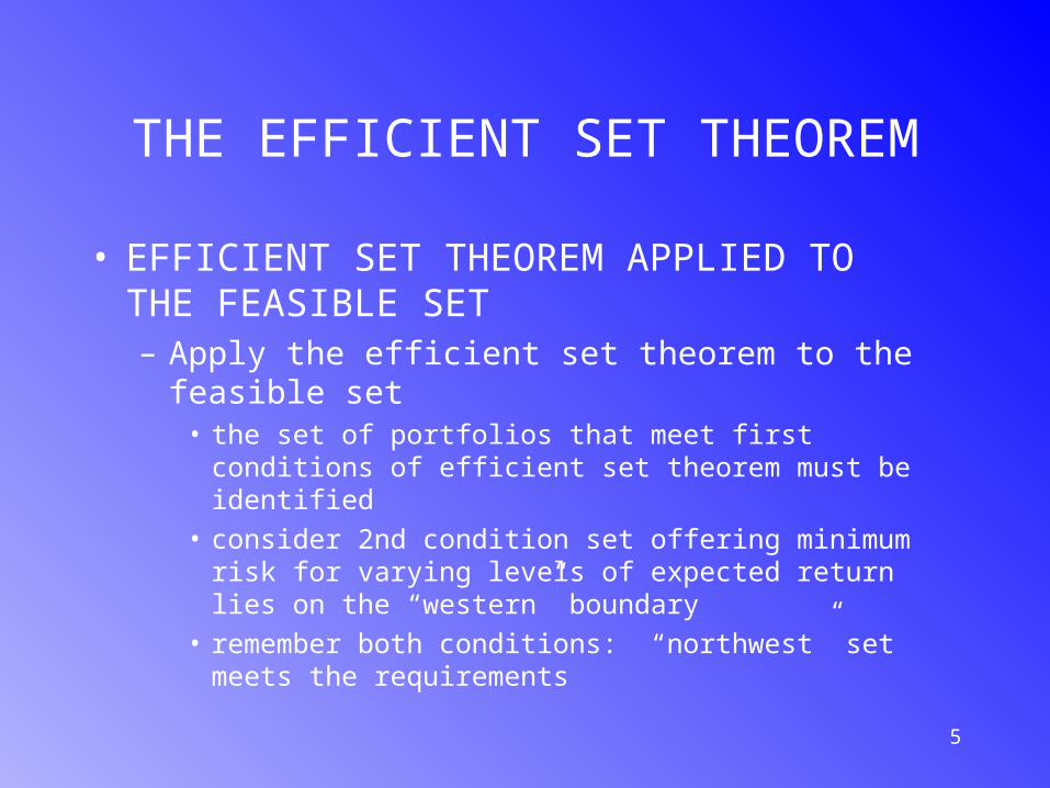
• EFFICIENT SET THEOREM APPLIED TO THE FEASIBLE SET– Apply the efficient set theorem to the feasible set
• the set of portfolios that meet first conditions of efficient set theorem must be identified
• consider 2nd condition set offering minimum risk for varying levels of expected return lies on the “western” boundary
• remember both conditions: “northwest” set meets the requirements

6
THE EFFICIENT SET THEOREM
• THE EFFICIENT SET– where the investor plots indifference curves and
chooses the one that is furthest “northwest”– the point of tangency at point E

7
THE EFFICIENT SET THEOREM
THE OPTIMAL PORTFOLIO
E
rP
P0
8
CONCAVITY OF THE EFFICIENT SET
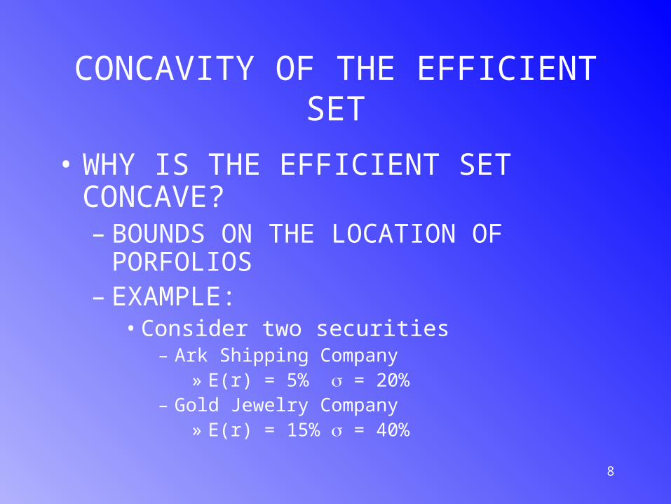
• WHY IS THE EFFICIENT SET CONCAVE?– BOUNDS ON THE LOCATION OF
PORFOLIOS– EXAMPLE:
• Consider two securities– Ark Shipping Company
» E(r) = 5% = 20%– Gold Jewelry Company
» E(r) = 15% = 40%
9
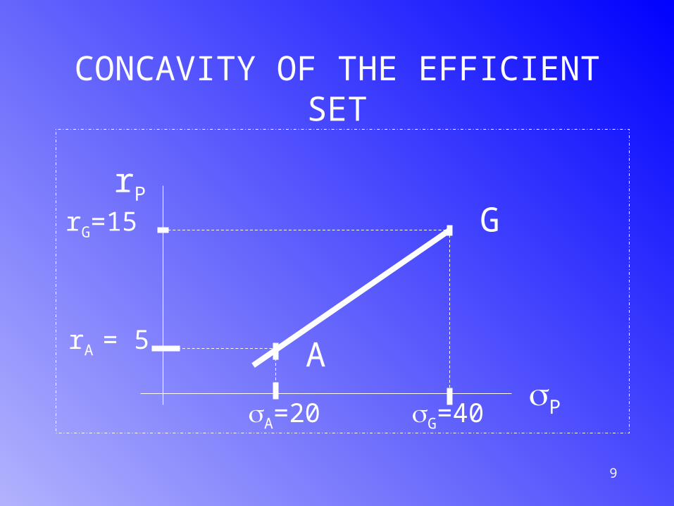
CONCAVITY OF THE EFFICIENT SET
P
rP
A
G
rA = 5
A=20
rG=15
G=40
10
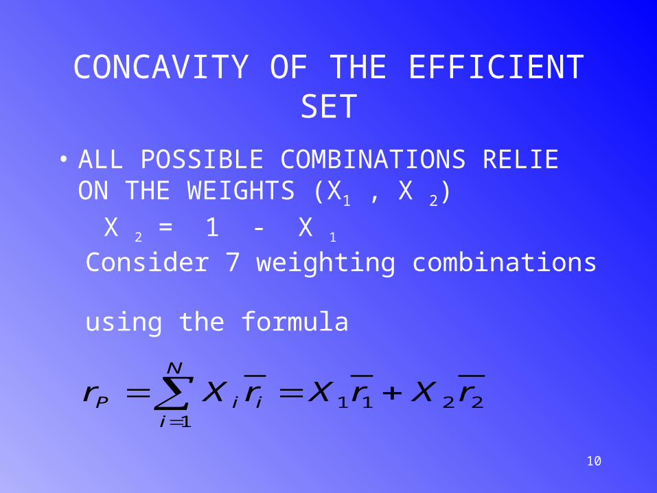
CONCAVITY OF THE EFFICIENT SET
• ALL POSSIBLE COMBINATIONS RELIE ON THE WEIGHTS (X1 , X 2)
X 2 = 1 - X 1
Consider 7 weighting combinations
using the formula
22111
rXrXrXrN
iiiP

11
CONCAVITY OF THE EFFICIENT SET
Portfolio return
A 5
B 6.7
C 8.3
D 10
E 11.7
F 13.3
G 15
12
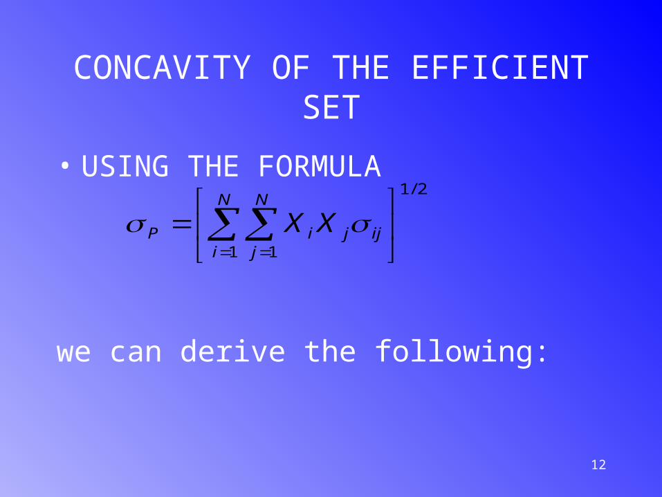
CONCAVITY OF THE EFFICIENT SET
• USING THE FORMULA
we can derive the following:
2/1
1 1
N
i
N
jijjiP XX
13
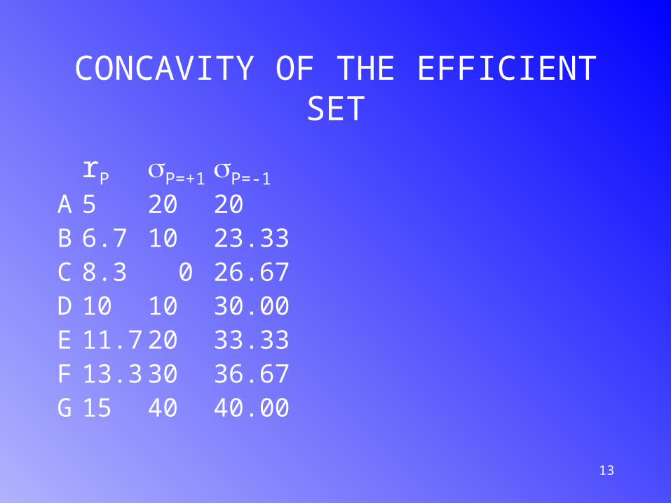
CONCAVITY OF THE EFFICIENT SET
rP P=+1 P=-1
A 5 20 20
B 6.7 10 23.33C 8.3 0 26.67D 10 10 30.00E 11.7 20 33.33F 13.3 30 36.67G 15 40 40.00
14
CONCAVITY OF THE EFFICIENT SET
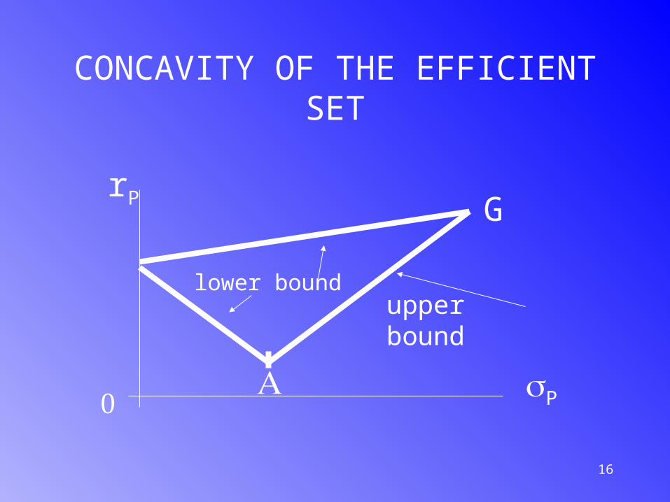
• UPPER BOUNDS– lie on a straight line connecting A and G
• i.e. all must lie on or to the left of the straight line
• which implies that diversification generally leads to risk reduction
15
CONCAVITY OF THE EFFICIENT SET
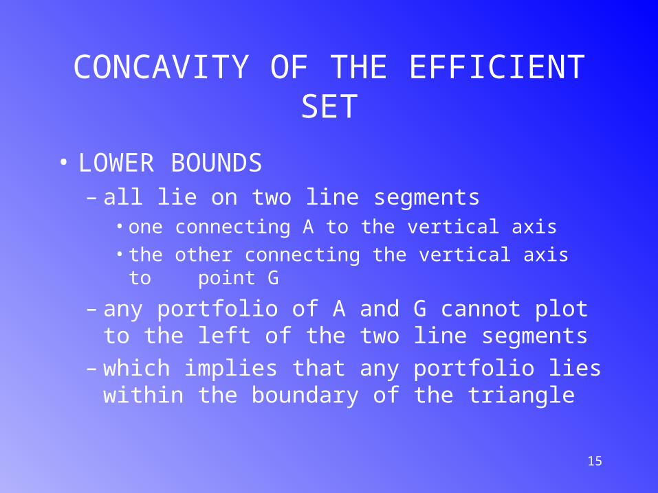
• LOWER BOUNDS– all lie on two line segments
• one connecting A to the vertical axis
• the other connecting the vertical axis to point G
– any portfolio of A and G cannot plot to the left of the two line segments
– which implies that any portfolio lies within the boundary of the triangle
16
CONCAVITY OF THE EFFICIENT SET
G
upper bound
lower bound
rP
P

17
CONCAVITY OF THE EFFICIENT SET
• ACTUAL LOCATIONS OF THE PORTFOLIO– What if correlation coefficient (ij ) is zero?

18
CONCAVITY OF THE EFFICIENT SET
RESULTS:
B = 17.94%
B = 18.81%
B = 22.36%
B = 27.60%
B = 33.37%

19
CONCAVITY OF THE EFFICIENT SET
ACTUAL PORTFOLIO LOCATIONS
CD
F
20
CONCAVITY OF THE EFFICIENT SET
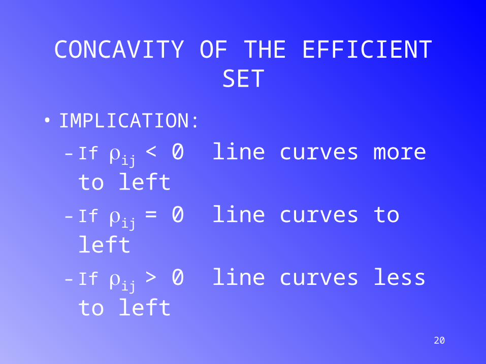
• IMPLICATION:
– If ij < 0 line curves more to left
– If ij = 0 line curves to left
– If ij > 0 line curves less to left
21
CONCAVITY OF THE EFFICIENT SET
• KEY POINT
– As long as -1 < the portfolio line curves to the left and the northwest portion is concave
– i.e. the efficient set is concave
22
THE MARKET MODEL
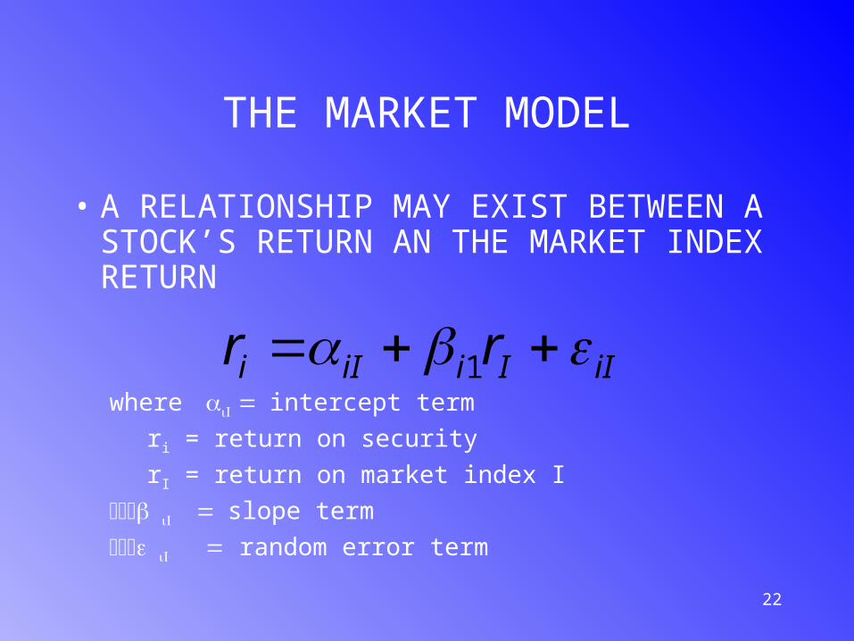
• A RELATIONSHIP MAY EXIST BETWEEN A STOCK’S RETURN AN THE MARKET INDEX RETURN
where intercept term
ri = return on security
rI = return on market index I
slope term
random error term
iIIiiIi rr 1
23
THE MARKET MODEL
• THE RANDOM ERROR TERMS i, I
– shows that the market model cannot explain perfectly
– the difference between what the actual return value is and
– what the model expects it to be is attributable to i, I

24
THE MARKET MODEL
i, I CAN BE CONSIDERED A RANDOM
VARIABLE
– DISTRIBUTION:• MEAN = 0
• VARIANCE = i
25
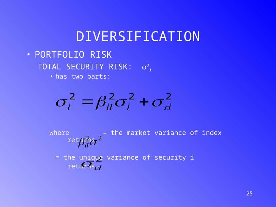
DIVERSIFICATION• PORTFOLIO RISK
TOTAL SECURITY RISK: i
• has two parts:
where = the market variance of index returns
= the unique variance of security i returns
2222iiiIi
22 iI2i
26
DIVERSIFICATION
• TOTAL PORTFOLIO RISK– also has two parts: market and unique
• Market Risk– diversification leads to an averaging of market risk
• Unique Risk– as a portfolio becomes more diversified, the smaller will
be its unique risk
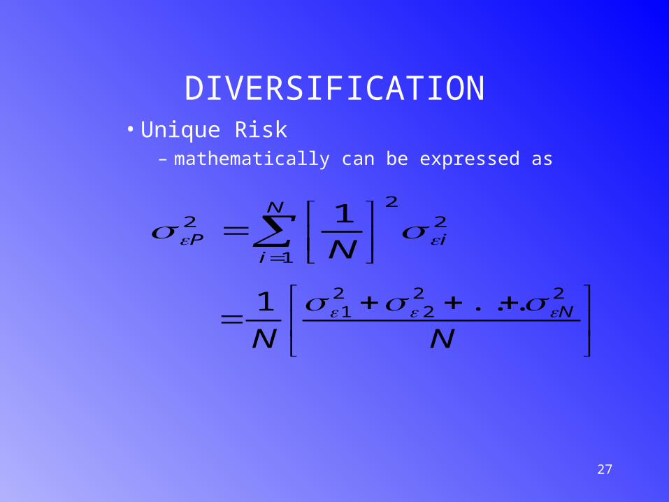
27
DIVERSIFICATION• Unique Risk
– mathematically can be expressed as
N
iiP N1
22
2 1
NNN
222
21 ...1