Chapter 11people.stat.sc.edu/hansont/stat704/Lecture18.pdfChapter11 Chapter 11 Timothy Hanson...

Chapter 11

Chapter 11

Timothy Hanson

Department of Statistics, University of South Carolina

Stat 704: Data Analysis I

1 / 23

Chapter 1111.1 Unequal variance rem. measure: Weighted least squares11.2 Multicollinearity rem. measure: Ridge regression

11.1: Weighted least squares

Chapters 3 and 6 discuss transformations of x1, . . . , xk and/orY .

This is “quick and dirty” but may not solve the problem.

Or can create an uninterpretable mess (book:“inappropriate”).

More advanced remedy: weighted least squares regression.

Model is as before

Yi = β0 + β1xi1 + · · ·βkxik + ǫi ,

but nowǫi

ind .∼ N(0, σ2

i ).

Note the subscript on σi ...

2 / 23


Here var(Yi ) = σ2i . Give observations with higher variance less

weight in the regression fitting.

Say σ1, . . . , σn are known. Let wi = 1/σ2i and define the

weight matrix

W =

w1 0 · · · 00 w2 · · · 0...

.... . .

...0 0 · · · wn

=

σ−21 0 · · · 0

0 σ−22 · · · 0

......

. . ....

0 0 · · · σ−2n

.

Maximizing the likelihood (pp. 422-423) gives the estimatesfor β:

bw = (XWX′)−1X′WY.

3 / 23


However, σ1, . . . , σn are almost always unknown.

If the mean function is appropriate, then E (e2i ) = σ2i (1− hii )

where ei is obtained from ordinary least squares, so e2iestimates σ2

i and |ei | estimates σi (pp. 424-425) as hii → 0 asn → ∞.

Look at plots of |ei | from a normal fit against predictors in themodel and the fitted values Yi to see how σi changes withpredictors or fitted values.

For example, if |ei | increases linearly with Yi = x′ib, then we’llfit |ei | = α0 + α1xi1 + · · ·+ αkxik + δi and obtain the fitted

values |ei |.

If e2i increases linearly with only xi4, then we’ll fit

e2i = α0 + α4xi4 + δi and obtain the fitted values e2i .

4 / 23


1 Regress Y against predictor variable(s) as usual (OLS) &obtain e1, . . . , en & Y1, . . . , Yn.

2 Regress |ei | against predictors x1, . . . , xk or fitted values Yi .

3 Let si be the fitted values for the regression in 2.

4 Define wi = 1/s2i for i = 1, . . . , n.

5 Use bw = (X′WX)−1X′WY as estimated coefficients –automatic in SAS. SAS will also use the correctcov(bw ) = (X′WX)−1 (p. 423). This is developed formally inlinear models.

5 / 23


SAS code: initial fit

* SAS example for Weighted Least Squares ;

* Blood pressure data in Table 11.1 ;

data bloodp; input age dbp @@; datalines;

27 73 21 66 22 63 24 75 25 71 23 70 20 65

20 70 29 79 24 72 25 68 28 67 26 79 38 91

32 76 33 69 31 66 34 73 37 78 38 87 33 76

35 79 30 73 31 80 37 68 39 75 46 89 49 101

40 70 42 72 43 80 46 83 43 75 44 71 46 80

47 96 45 92 49 80 48 70 40 90 42 85 55 76

54 71 57 99 52 86 53 79 56 92 52 85 50 71

59 90 50 91 52 100 58 80 57 109

; run;

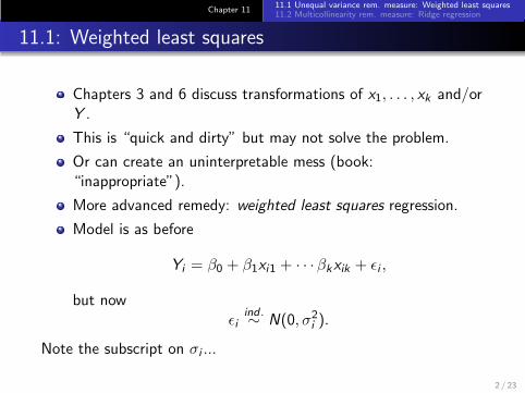
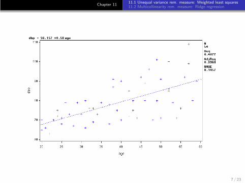
* Regress the response, dbp, against the predictor, age ;

* The plots show definite nonconstant error variance ;

proc reg data=bloodp;

model dbp=age;

output out=temp r=residual;

plot dbp*age r.*age;

run;

6 / 23


7 / 23


8 / 23


SAS code: determining wi

* Plot of absolute residuals against age shows that

absolute residuals increase approximately linearly;

data temp; set temp; absr = abs(residual); run;

symbol1 v=dot h=0.8;

axis1 order=(0 to 20 by 5);

proc gplot data=temp; PLOT absr*age/ vaxis=axis1; run;

9 / 23


SAS code: WLS fit

* Regress absolute residuals against the age ;

* This second regression is done on the data set temp ;

proc reg data=temp;

model absr=age;

output out=temp1 p=s_hat ;

run;

* Define weights using the fitted values from this second regression ;

data temp1; set temp1; w=1/(s_hat**2); run;

* Using the WEIGHT option in PROC REG to get the WLS estimates ;

* This last regression is done on the data set temp1 ;

proc reg data=temp1;

weight w;

model dbp=age / clb;

output out=temp2 r=residual;

plot dbp*age r.*age;

run;

10 / 23


SAS output: WLS fit

The REG Procedure

Dependent Variable: dbp

Weight: w

Analysis of Variance

Sum of Mean

Source DF Squares Square F Value Pr > F

Model 1 83.34082 83.34082 56.64 <.0001

Error 52 76.51351 1.47141

Corrected Total 53 159.85432

Root MSE 1.21302 R-Square 0.5214

Dependent Mean 73.55134 Adj R-Sq 0.5122

Coeff Var 1.64921

Parameter Estimates

Parameter Standard

Variable DF Estimate Error t Value Pr > |t| 95% Confidence Limits

Intercept 1 55.56577 2.52092 22.04 <.0001 50.50718 60.62436

age 1 0.59634 0.07924 7.53 <.0001 0.43734 0.75534

11 / 23


se(b1) reduced from 0.097 (OLS) to 0.079 (WLS). WLSverified via bootstrap on pp. 462–463 (just FYI).

R2 no longer interpreted the same way in terms of amount oftotal variability explained by model.

In WLS, standard inferences about coefficients may not bevalid for small sample sizes when weights are estimated fromthe data.

If MSE of the WLS regression is near 1, then our estimation ofthe “error standard deviation” function is okay. Here it’s 1.21.

12 / 23


Fitting the model directly...

A drawback of this approach is that the weights wi = 1/s2ihave associated variability that is not reflected in cov(bw ).

It is possible to fit the implied model

Yi = β0 + β1ai + ǫi , ǫi ∼ N(0, τ0 + τ1ai ),

directly in SAS. One option is to have SAS maximize theassociated likelihood in PROC NLMIXED.

Note that a similar, and possibly more appropriate, model

Yi = β0 + β1ai + ǫi , ǫi ∼ N(0, eτ0+τ1ai ),

was used for the Breusch-Pagan test H0 : τ1 = 0 described inSections 3.6 and 6.8. This model can also be fit easily inPROC NLMIXED.

However, things like F -tests go out the window andeverything relies on asymptotics (which for large enoughsamples work fine).

13 / 23


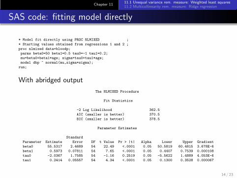
SAS code: fitting model directly

* Model fit directly using PROC NLMIXED ;

* Starting values obtained from regressions 1 and 2 ;

proc nlmixed data=bloodp;

parms beta0=50 beta1=0.5 tau0=-1 tau1=0.2;

mu=beta0+beta1*age; sigma=tau0+tau1*age;

model dbp ~ normal(mu,sigma*sigma);

run;

With abridged output

The NLMIXED Procedure

Fit Statistics

-2 Log Likelihood 362.5

AIC (smaller is better) 370.5

BIC (smaller is better) 378.5

Parameter Estimates

Standard

Parameter Estimate Error DF t Value Pr > |t| Alpha Lower Upper Gradient

beta0 55.5317 2.4689 54 22.49 <.0001 0.05 50.5819 60.4815 3.678E-6

beta1 0.5973 0.07811 54 7.65 <.0001 0.05 0.4407 0.7539 0.000108

tau0 -2.0367 1.7585 54 -1.16 0.2519 0.05 -5.5622 1.4889 4.053E-6

tau1 0.2414 0.05557 54 4.34 <.0001 0.05 0.1300 0.3528 0.000067

14 / 23


11.2: Ridge regression

Before considering ridge regression, recall that even serious

multicollinearity does not present a problem when the focus ison prediction, and prediction is limited to the overall patternof predictors in the data. Use x′h(X

′X)−1xh for predictor xhand compare to the rest of the leverages.

Principle components provide composite “predictors” that areuncorrelated. Under umbrella term of “dimension reduction.”

Ridge regression is an advanced remedial measure formulticollinearity that uses a biased estimate bR instead of theOLS b.

Although biased, it may have less variance – one of the effectsof multicollinearity was exploding se(bk). See Fig. 11.2 (p.432).

15 / 23


Ridge regression adds a biasing constant c to the normalequations based on the standardized regression modeldeveloped in Section 7.5 (also used for VIFs in 10.5); read pp.273–275 and p. 433.

c = 0 ⇒ OLS estimator b.

Bias in the estimator bR increases/decreases with c .

VIFs/R2 decrease with increasing c .

Look at plots of bRj and VIFj versus c to see when estimatesand variance inflation stabilize. Can get these automatically inSAS.

Note no standard errors when choosing c by eye. Need to usebootstrap; not automatic in SAS.

Ridge regression is related to the LASSO; more in a minute...

16 / 23


Standard error for fixed c

Page 433. Working with standardized model

Y ∗

i = β∗

1x∗

i1 + · · ·β∗

kx∗

ik + ǫ∗i .

bR = ((X∗)′X∗ + cI)−1(X∗)′Y∗.

So

cov(bR) = ((X∗)′X∗ + cI)−1k (X∗)′(X∗)((X∗)′X∗ + cI)−1(σ∗)2.

Why not output from SAS?Note: Ridge regression gives the same estimate as the Bayesianposterior mode of β∗ under independent mean-zero normal priorswith variance τ2 on the β∗

1 , . . . , β∗

k . Here, c = (σ∗)2/τ2.

17 / 23


SAS code & output: body fat data

*******************************

* Body fat data from Chapter 7

*******************************;

data body;

input triceps thigh midarm bodyfat @@;

cards;

19.5 43.1 29.1 11.9 24.7 49.8 28.2 22.8

30.7 51.9 37.0 18.7 29.8 54.3 31.1 20.1

19.1 42.2 30.9 12.9 25.6 53.9 23.7 21.7

31.4 58.5 27.6 27.1 27.9 52.1 30.6 25.4

22.1 49.9 23.2 21.3 25.5 53.5 24.8 19.3

31.1 56.6 30.0 25.4 30.4 56.7 28.3 27.2

18.7 46.5 23.0 11.7 19.7 44.2 28.6 17.8

14.6 42.7 21.3 12.8 29.5 54.4 30.1 23.9

27.7 55.3 25.7 22.6 30.2 58.6 24.6 25.4

22.7 48.2 27.1 14.8 25.2 51.0 27.5 21.1

;

run;

proc reg data=body outest=ridge outvif ridge=0.01 to 0.5 by .01;

model bodyfat=triceps thigh midarm;

plot / ridgeplot; run;

* I would probably take c=0.1 or c=0.2 based on the plot;

proc print; run;

proc reg data=body outest=ridge ridge=0.2;

model bodyfat=triceps thigh midarm; run;

proc print data=ridge; run;

Obs _MODEL_ _TYPE_ _DEPVAR_ _RIDGE_ _PCOMIT_ _RMSE_ Intercept triceps thigh midarm bodyfat

1 MODEL1 PARMS bodyfat . . 2.47998 117.085 4.33409 -2.85685 -2.18606 -1

2 MODEL1 RIDGE bodyfat 0.2 . 2.65543 -9.202 0.39789 0.42405 -0.08581 -118 / 23


19 / 23


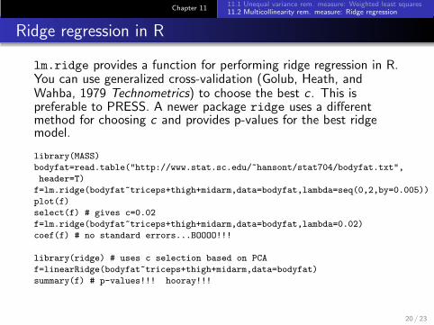
Ridge regression in R

lm.ridge provides a function for performing ridge regression in R.You can use generalized cross-validation (Golub, Heath, andWahba, 1979 Technometrics) to choose the best c . This ispreferable to PRESS. A newer package ridge uses a differentmethod for choosing c and provides p-values for the best ridgemodel.

library(MASS)

bodyfat=read.table("http://www.stat.sc.edu/~hansont/stat704/bodyfat.txt",

header=T)

f=lm.ridge(bodyfat~triceps+thigh+midarm,data=bodyfat,lambda=seq(0,2,by=0.005))

plot(f)

select(f) # gives c=0.02

f=lm.ridge(bodyfat~triceps+thigh+midarm,data=bodyfat,lambda=0.02)

coef(f) # no standard errors...BOOOO!!!

library(ridge) # uses c selection based on PCA

f=linearRidge(bodyfat~triceps+thigh+midarm,data=bodyfat)

summary(f) # p-values!!! hooray!!!

20 / 23


Penalized least-squares (p. 436) formulation of ridge regression:

Qpen =n∑

i=1

(Y ∗

i − (x∗i )′bR)2 + c

k∑

j=1

(bRj )2.

The solution is bR that minimizes Qpen.

21 / 23


LASSO chooses bL to minimize

n∑

i=1

(Y ∗

i − (x∗i )′bL)2 + c

k∑

j=1

|bLj |

In LASSO, this constraint leads to some bLj ’s set exactly to zero,so LASSO can be viewed as a method of variable selection as wellas coefficient estimation.

Traditionally ridge regression estimates have been easier to obtain(computationally) than LASSO estimates. However, recentadvances allow for the routine use of LASSO. LASSO for variableselection is in the new SAS PROC GLMSELECT.

22 / 23


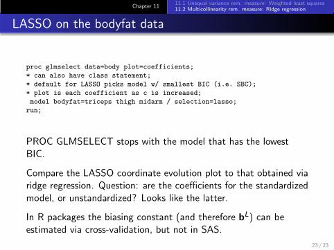
LASSO on the bodyfat data

proc glmselect data=body plot=coefficients;

* can also have class statement;

* default for LASSO picks model w/ smallest BIC (i.e. SBC);

* plot is each coefficient as c is increased;

model bodyfat=triceps thigh midarm / selection=lasso;

run;

PROC GLMSELECT stops with the model that has the lowestBIC.

Compare the LASSO coordinate evolution plot to that obtained viaridge regression. Question: are the coefficients for the standardizedmodel, or unstandardized? Looks like the latter.

In R packages the biasing constant (and therefore bL) can beestimated via cross-validation, but not in SAS.

23 / 23

Chapter 11people.stat.sc.edu/hansont/stat704/Lecture18.pdfChapter11 Chapter 11 Timothy Hanson...

Documents

Transcript of Chapter 11people.stat.sc.edu/hansont/stat704/Lecture18.pdfChapter11 Chapter 11 Timothy Hanson...