Chapter 9

Zonotopes

“And what is the use of a book,” thought Alice, “without pictures or conversations?”

Lewis Carroll (Alice in Wonderland)

We have seen that the discrete volume of a general integral polytope maybe quite di�cult to compute. It is therefore useful to have an infinite classof integral polytopes such that their discrete volume is more tractable, andyet they are robust enough to be “closer” in complexity to generic integralpolytopes. One initial class of more tractable polytopes are parallelepipeds,and as we will see in Lemma 9.2, the Ehrhart polynomial of a d-dimensionalhalf-open integer parallelepiped P is equal to vol(P) td. In this chapter, wegeneralize parallelepipeds to projections of cubes.

9.1 Definitions and Examples

In order to extend the notion of a parallelepiped, we begin by defining theMinkowski sum of the polytopes P

1

,P2

, . . . ,Pn

⇢ Rd as

P1

+ P2

+ · · ·+ Pn

:= {x1

+ x2

+ · · ·+ xn

: xj

2 Pj

} .

For example, if P1

is the rectangle [0, 2] ⇥ [0, 1] ⇢ R2 and P2

is the linesegment

⇥�

0

0

�

,�

2

3

�⇤ ⇢ R2, then their Minkowski sum P1

+ P2

is the hexagon

whose vertices are�

0

0

�

,�

2

0

�

,�

0

1

�

,�

4

3

�

,�

2

4

�

, and�

4

4

�

, as depicted in Figure 9.1.Parallelepipeds are special instances of Minkowski sums, namely those of linesegments whose direction vectors are linearly independent, plus a point.

We will also make use of the following handy construct: Given a polynomialp(z

1

, z2

, . . . , zd

) in d variables, the Newton polytope N (p(z1

, z2

, . . . , zd

))of p(z

1

, z2

, . . . , zd

) is the convex hull of all exponent vectors appearing in the

165

166 9 Zonotopes

+ =

Fig. 9.1 The Minkowski sum ([0, 2]⇥ [0, 1]) +⇥�0

0

�,�23

�⇤.

nonzero terms of p(z1

, z2

, . . . , zd

). For example, the hexagon in Figure 9.1 canbe written as

N �

1 + 3z21

� z2

� 5z41

z32

+ 34z21

z42

+ z41

z42

�

.

It turns out (Exercise 9.1) that the constructions of Newton polytopesand Minkowski sums are intimately related. Namely, if p(z

1

, z2

, . . . , zd

) andq(z

1

, z2

, . . . , zd

) are polynomials, then

N �

p(z1

, z2

, . . . , zd

) q(z1

, z2

, . . . , zd

)�

= N �

p(z1

, z2

, . . . , zd

)�

+N �

q(z1

, z2

, . . . , zd

)�

. (9.1)

Suppose that we are now given n line segments in Rd, such that each linesegment has one endpoint at the origin and the other endpoint is located atthe vector u

j

2 Rd, for j = 1, . . . , n. Then by definition, the Minkowski sumof these n segments is

Z(u1

,u2

, . . . ,un

) := {x1

+ x2

+ · · ·+ xn

: xj

= �j

uj

with �j

2 [0, 1]} .

Fig. 9.2 The zono-tope Z

��04

�,�33

�,�41

��—a

hexagon.

Let’s rewrite the definition above in matrix form:

9.1 Definitions and Examples 167

Z(u1

,u2

, . . . ,un

) = {�1

u1

+ �2

u2

+ · · ·+ �n

un

: 0 �j

1}

=

8

>

>

>

<

>

>

>

:

(u1

u2

· · · un

)

0

B

B

B

@

�1

�2

...�n

1

C

C

C

A

: 0 �j

1

9

>

>

>

=

>

>

>

;

= A [0, 1]n,

where A is the (d ⇥ n)-matrix whose j’th column is uj

. Just a bit moregenerally, a zonotope is defined to be any translate of A [0, 1]n, i.e.,

A [0, 1]n + b ,

for some vector b 2 Rd. So we now have two equivalent definitions of azonotope—the first one is given by a Minkowski sum of line segments, whilethe second one is given by any projection of the unit cube [0, 1]n. Figures 9.2and 9.3 show two example zonotopes.

Fig. 9.3 The rhombic do-decahedron is a zonotope.

It is sometimes useful to translate a zonotope so that the origin becomesits new center of mass. To this end, we now dilate the matrix A by a factorof 2 and translate the resulting image so that its new center of mass is at theorigin. Precisely, we have

2A [0, 1]n � (u1

+ · · ·+ un

)

= {2u1

�1

+ · · ·+ 2un

�n

� (u1

+ · · ·+ un

) : 0 �j

1}= {u

1

(2�1

� 1) + · · ·+ un

(2�n

� 1) : 0 �j

1}= A [�1, 1]n, (9.2)

where the last step holds because �1 2�j

� 1 1 when 0 �j

1. Inother words, (9.2) is a linear image of the larger cube [�1, 1]n, centered atthe origin. We thus define

168 9 Zonotopes

Z(±u1

,±u2

, . . . ,±un

) := A [�1, 1]n,

and we see that Z(±u1

,±u2

, . . . ,±un

) is indeed a zonotope, by definition.We say that a polytope P is symmetric about the origin when it has theproperty that x 2 P if and only if �x 2 P . In general, a polytope P is calledcentrally symmetric if we can translate P by some vector b such thatP + b is symmetric about the origin. The zonotope Z(±u

1

,±u2

, . . . ,±un

)is an example of a polytope that is symmetric about the origin. We gothrough the clean argument here, because it justifies our choice of a symmetricrepresentation: Pick any x 2 Z(±u

1

,±u2

, . . . ,±un

), so that x = Ay, withy 2 [�1, 1]n. Since �y 2 [�1, 1]n as well, we have

�x = A (�y) 2 Z(±u1

,±u2

, . . . ,±un

) .

It is moreover true that each face of a zonotope is again a zonotope and thattherefore every face of a zonotope is centrally symmetric (Exercise 9.2).

Fig. 9.4 A few more zonotopes.

9.2 Paving a Zonotope

Next we will show that any zonotope can be neatly decomposed into a disjointunion of half-open parallelepipeds. Suppose that w

1

,w2

, . . . ,wm

2 Rd arelinearly independent, and let �

1

,�2

, . . . ,�m

2 {±1}. Then we define

⇧�1,�2,...,�m

w1,w2,...,wm

:=

⇢

�1

w1

+ �2

w2

+ · · ·+ �m

wm

:0 �

j

< 1 if �j

= �10 < �

j

1 if �j

= 1

�

.

In plain English, ⇧�1,�2,...,�m

w1,w2,...,wm

is a half-open parallelepiped generated byw

1

,w2

, . . . ,wm

, and the signs �1

,�2

, . . . ,�m

keep track of those facets ofthe parallelepiped that are included or excluded from the closure of theparallelepiped.

9.2 Paving a Zonotope 169

Lemma 9.1. The zonotope Z(u1

,u2

, . . .un

) can be written as a disjointunion of translates of ⇧�1,�2,...,�m

w1,w2,...,wm

, where {w1

,w2

, . . . ,wm

} ranges overall linearly independent subsets of {u

1

,u2

, . . .un

}, each equipped with anappropriate choice of signs �

1

,�2

, . . . ,�m

.

Figure 9.5 illustrates the decomposition of a zonotope as suggested byLemma 9.1.

Fig. 9.5 A zonotopal decomposition of Z��0

4

�,�33

�,�41

��.

Proof of Lemma 9.1. We proceed by induction on n. If n = 1, Z(u1

) is a linesegment and 0 [ (0,u

1

] is a desired decomposition.For general n > 1, we have by induction the decomposition

Z(u1

,u2

, . . . ,un�1

) = ⇧1

[⇧2

[ · · · [⇧k

into half-open parallelepipeds of the form given in the statement of Lemma 9.1.Now we define the hyperplane H := {x 2 Rd : x ·u

n

= 0} and let ⇡ : Rd ! Hdenote the orthogonal projection onto H . Then ⇡(u

1

),⇡(u2

), . . . ,⇡(un�1

) areline segments or points, and thus Z(⇡(u

1

),⇡(u2

), . . . ,⇡(un�1

)) is a zonotopeliving in H. Once more by induction we can decompose

Z(⇡(u1

),⇡(u2

), . . . ,⇡(un�1

)) = �1

[ �2

[ · · · [ �m

into half-open parallelepipeds of the form given in Lemma 9.1. Each �j

is ahalf-open parallelepiped generated by some of the vectors ⇡(u

1

), ⇡(u2

), . . . ,⇡(u

n�1

); let e�j

denote the corresponding parallelepiped generated by theirnon-projected counterparts. Then (Exercise 9.5) the desired disjoint union ofZ(u

1

,u2

, . . . ,un

) is given by ⇧1

[⇧2

[ · · · [⇧k

[ P1

[ P2

[ · · · [ Pm

where

170 9 Zonotopes

Pj

:= e�j

⇥ (0,un

] . ut

This decomposition lemma is useful, e.g., to compute the Ehrhart polyno-mial of a zonotope. To this end, we now first work out the Ehrhart polynomialof a half-open parallelepiped, which in itself is a (particularly simple) zonotope.

Lemma 9.2. Suppose w1

,w2

, . . . ,wd

2 Zd are linearly independent, and let

⇧ := {�1

w1

+ �2

w2

+ · · ·+ �d

wd

: 0 �1

,�2

, . . . ,�d

< 1} .

Then#�

⇧ \ Zd

�

= vol⇧ = |det (w1

, . . . ,wd

)| ,and for any positive integer t,

#�

t⇧ \ Zd

�

= (vol⇧) td.

In other words, for the half-open parallelepiped ⇧, the discrete volume#�

t⇧ \ Zd

�

coincides with the continuous volume (vol⇧) td.

Proof. Because ⇧ is half open, we can tile the tth dilate t⇧ by td translatesof ⇧, and hence

L⇧

(t) = #�

t⇧ \ Zd

�

= #�

⇧ \ Zd

�

td.

On the other hand, by the results of Chapter 3, L⇧

(t) is a polynomial withleading coe�cient vol⇧ = |det (w

1

, . . . ,wd

)|. Since we have equality of thesepolynomials for all positive integers t,

#�

⇧ \ Zd

�

= vol⇧ . ut

Our proof shows that Lemma 9.2 remains true if we switch the and <inequalities for some of the �

j

in the definition of ⇧, a fact that we will usefreely, e.g., in the following tool to compute Ehrhart polynomials of zonotopes,which follows from a combination of Lemmas 9.1 and 9.2.

Corollary 9.3. Decompose the zonotope Z ⇢ Rd into half-open parallelepipedsaccording to Lemma 9.1. Then the coe�cient c

k

of the Ehrhart polynomialLZ(t) = c

d

td + cd�1

td�1 + · · ·+ c0

equals the sum of the (relative) volumesof the k-dimensional parallelepipeds in the decomposition of Z.

9.3 The Permutahedron

To illustrate that Corollary 9.3 is useful for computations, we now study afamous polytope, the permutahedron

Pd

:= conv {(⇡(1)� 1, ⇡(2)� 1, . . . , ⇡(d)� 1) : ⇡ 2 Sd

} ,

9.3 The Permutahedron 171

that is, the convex hull of (0, 1, . . . , d�1) and all points formed by permuting itsentries. It is not hard to show (see Exercise 9.9) that P

d

is (d�1)-dimensionaland has d! vertices. Figures 9.6 and 9.7 show P

3

and P4

(as the latter isprojected into R3).

Fig. 9.6 The permutahe-dron P3.

x

y

z

(0, 2, 1)

(1, 2, 0)

(2, 1, 0)

(2, 0, 1)

(1, 0, 2)

(0, 1, 2)

The reason that permutahedra make an appearance in this chapter is thefollowing result.

Theorem 9.4.

Pd

= [e1

, e2

] + [e1

, e3

] + · · ·+ [ed�1

, ed

] ,

in words: the permutahedron Pd

is the Minkowski sum of the line segmentsbetween each pair of unit vectors in Rd.

Proof. We make use of a matrix that already made its debut in Section 3.7:namely, the permutahedron P

d

is the Newton polytope of the polynomial

det

0

B

B

B

@

xd�1

1

xd�2

1

· · · x1

1xd�1

2

xd�2

2

· · · x2

1...

......

...xd�1

d

xd�2

d

· · · xd

1

1

C

C

C

A

—one can see the vertices of Pd

appearing in the exponent vectors bycomputing this determinant by cofactor expansion. Now we use Exercise 3.20:

det

0

B

B

B

@

xd�1

1

xd�2

1

· · · x1

1xd�1

2

xd�2

2

· · · x2

1...

......

...xd�1

d

xd�2

d

· · · xd

1

1

C

C

C

A

=Y

1j<kd

(xj

� xk

) ,

172 9 Zonotopes

(0, 1, 2, 3)

(1, 0, 2, 3)

(1, 0, 3, 2)

(0, 1, 3, 2)

(0, 2, 1, 3)

(2, 0, 1, 3)

(2, 1, 0, 3)

(1, 2, 0, 3)

(0, 2, 3, 1)

(0, 3, 2, 1)

(0, 3, 1, 2)

(3, 0, 1, 2)

(3, 1, 0, 2)

(1, 3, 0, 2)

(1, 3, 2, 0)

(1, 2, 3, 0)

(2, 0, 3, 1)

(2, 3, 0, 1)

(2, 3, 1, 0)

(2, 1, 3, 0)

(3, 2, 0, 1)

(3, 0, 2, 1)

(3, 2, 1, 0)

(3, 1, 2, 0)

Fig. 9.7 The permutahedron P4 (projected into R3).

and so by (9.1) we have

Pd

= N (x1

� x2

) +N (x1

� x3

) + · · ·+N (xd�1

� xd

) .

The right-hand side is the Minkowski sum of the line segments [e1

, e2

], [e1

, e3

],. . . , [e

d�1

, ed

]. utNow we will apply Corollary 9.3 to the special zonotope P

d

. A forest is agraph that does not contain any closed paths.

Theorem 9.5. The coe�cient ck

of the Ehrhart polynomial

LPd

(t) = cd�1

td�1 + cd�2

td�2 + · · ·+ c0

of the permutahedron Pd

equals the number of labeled forests on d nodes withk edges.

For example, we can compute LP3(t) = 3t2 + 3t + 1 by looking at thelabeled forests in Figure 9.8.

An important ingredient to the proof of Theorem 9.5 is the following cor-respondence: to a subset S ✓ {e

1

+ e2

, e1

+ e3

, . . . , ed�1

+ ed

} we associatethe graph G

S

with node set [d] and edge set

{jk : ej

+ ek

2 S} .

We invite the reader to prove (Exercise 9.12):

9.3 The Permutahedron 173

Fig. 9.8 The 3 + 3 + 1labeled forests on threenodes.

Lemma 9.6. A subset S ✓ {e1

+ e2

, e1

+ e3

, . . . , ed�1

+ ed

} is linearly inde-pendent if and only if G

S

is a forest.

Proof of Theorem 9.5. Let I consist of all nonempty linearly independentsubsets of

{e1

+ e2

, e1

+ e3

, . . . , ed�1

+ ed

} .To each such subset S we will associate the half-open parallelepiped

X

e

j

+e

k

2S

(0, ej

+ ek

]

(written as a Minkowski sum). It has relative volume 1 (Exercise 9.13). Thesehalf-open parallelepipeds give rise to the disjoint union

Pd

= Z (e1

+ e2

, e1

+ e3

, . . . , ed�1

+ ed

)

= 0 [[

S2I

0

@

X

e

j

+e

k

2S

(0, ej

+ ek

]

1

A , (9.3)

as the reader should verify in Exercise 9.14. Corollary 9.3 now says that thecoe�cient c

k

of the Ehrhart polynomial

LPd

(t) = cd�1

td�1 + cd�2

td�2 + · · ·+ c0

equals the sum of the relative volumes of the k-dimensional parallelepipeds inour zonotopal decomposition of P

d

given in (9.3). As mentioned above, eachof these volumes is 1, and Lemma 9.6 now gives the statement of Theorem 9.5.

ut

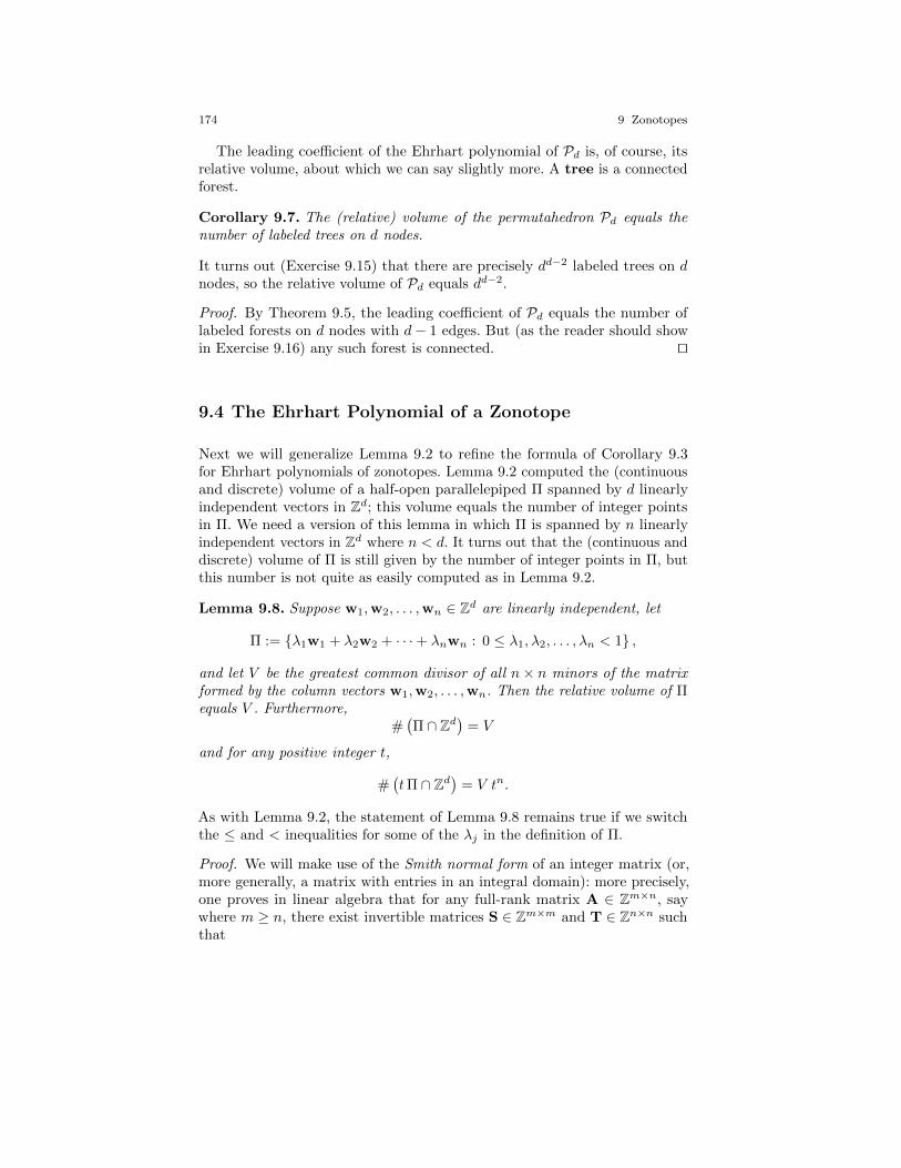
174 9 Zonotopes

The leading coe�cient of the Ehrhart polynomial of Pd

is, of course, itsrelative volume, about which we can say slightly more. A tree is a connectedforest.

Corollary 9.7. The (relative) volume of the permutahedron Pd

equals thenumber of labeled trees on d nodes.

It turns out (Exercise 9.15) that there are precisely dd�2 labeled trees on dnodes, so the relative volume of P

d

equals dd�2.

Proof. By Theorem 9.5, the leading coe�cient of Pd

equals the number oflabeled forests on d nodes with d� 1 edges. But (as the reader should showin Exercise 9.16) any such forest is connected. ut

9.4 The Ehrhart Polynomial of a Zonotope

Next we will generalize Lemma 9.2 to refine the formula of Corollary 9.3for Ehrhart polynomials of zonotopes. Lemma 9.2 computed the (continuousand discrete) volume of a half-open parallelepiped ⇧ spanned by d linearlyindependent vectors in Zd; this volume equals the number of integer pointsin ⇧. We need a version of this lemma in which ⇧ is spanned by n linearlyindependent vectors in Zd where n < d. It turns out that the (continuous anddiscrete) volume of ⇧ is still given by the number of integer points in ⇧, butthis number is not quite as easily computed as in Lemma 9.2.

Lemma 9.8. Suppose w1

,w2

, . . . ,wn

2 Zd are linearly independent, let

⇧ := {�1

w1

+ �2

w2

+ · · ·+ �n

wn

: 0 �1

,�2

, . . . ,�n

< 1} ,

and let V be the greatest common divisor of all n⇥ n minors of the matrixformed by the column vectors w

1

,w2

, . . . ,wn

. Then the relative volume of ⇧equals V . Furthermore,

#�

⇧ \ Zd

�

= V

and for any positive integer t,

#�

t⇧ \ Zd

�

= V tn.

As with Lemma 9.2, the statement of Lemma 9.8 remains true if we switchthe and < inequalities for some of the �

j

in the definition of ⇧.

Proof. We will make use of the Smith normal form of an integer matrix (or,more generally, a matrix with entries in an integral domain): more precisely,one proves in linear algebra that for any full-rank matrix A 2 Zm⇥n, saywhere m � n, there exist invertible matrices S 2 Zm⇥m and T 2 Zn⇥n suchthat

9.4 The Ehrhart Polynomial of a Zonotope 175

SAT =

0

B

B

B

B

B

B

B

B

B

B

B

B

@

d1

0 · · · 00 d

2

.... . .

...dn�1

00 · · · 0 d

n

0 · · · 0...

...0 · · · 0

1

C

C

C

C

C

C

C

C

C

C

C

C

A

with diagonal integer entries whose product d1

d2

· · · dn

equals the gcd of alln⇥ n minors of A.

Geometrically, our matrices S and T transform ⇧ into the half-openrectangular parallelepiped

e⇧ := [0, d1

)⇥ [0, d2

)⇥ · · ·⇥ [0, dn

) ⇢ Rd

in such a way that the integer lattice Zd is preserved; in particular, the relativevolumes of ⇧ and e⇧ are equal, namely d

1

d2

· · · dn

= V . Furthermore,

#�

⇧ \ Zd

�

= #⇣

e⇧ \ Zd

⌘

= d1

d2

· · · dn

= V.

The remainder of our proof follows that of Lemma 9.2: since ⇧ is half open,we can tile the tth dilate t⇧ by tn translates of ⇧, and so

#�

t⇧ \ Zd

�

= #�

⇧ \ Zd

�

tn. ut

Lemma 9.8 is the crucial ingredient for the following refinement of Corollary9.3.

Theorem 9.9. Let Z := Z(u1

, . . . ,un

) be a zonotope generated by the integervectors u

1

, . . . ,un

. Then the Ehrhart polynomial of Z is given by

LZ(t) =X

S

m(S) t|S|,

where S ranges over all linearly independent subsets of {u1

, . . . ,un

}, andm(S) is the greatest common divisor of all minors of size |S| of the matrixwhose columns are the elements of S.

For example, going to back to the zonotope Z ��

0

4

�

,�

3

3

�

,�

4

1

��

featured inFigure 9.5, we compute

LZ((04),(33),(

41))

(t) =

�

�

�

�

det

✓

0 34 3

◆

�

�

�

�

t2 +

�

�

�

�

det

✓

0 44 1

◆

�

�

�

�

t2 +

�

�

�

�

det

✓

3 43 1

◆

�

�

�

�

t2

+ gcd(0, 4) t+ gcd(3, 3) t+ gcd(4, 1) t+ 1

= 37 t2 + 8 t+ 1 .

176 9 Zonotopes

We remark that the numbers m(S) appearing in Theorem 9.9 have ge-ometric meaning: If V (S) and L(S) denote the vector space and latticegenerated by S, respectively, then m(S) equals the cardinality of the group�

V (S) \ Zd

�

/L(S).

Proof of Theorem 9.9. Decompose Z as described in Lemma 9.1. Corollary9.3 says that the coe�cient c

k

of the Ehrhart polynomial

LZ(t) = cd

td + cd�1

td�1 + · · ·+ c0

equals the sum of the relative volumes of the k-dimensional parallelepipedsin this decomposition. Lemma 9.8 implies that these relative volumes arethe gcd’s of the minors of the matrices formed by the generators of theseparallelepipeds. ut

Notes

1. The word “zonotope” appears to have originated from the fact that for eachline segment u

j

that comes into the Minkowski-sum definition of a zonotopeZ, there corresponds a “zone,” composed of all of the facets of Z that containparallel translates of u

j

. This zone separates the zonotope into two isometricpieces, a “northern” hemisphere and a “southern” hemisphere, a propertythat is sometimes useful in their study.

2. The combinatorial study of zonotopes was brought to the forefront (if notinitiated) by Peter McMullen [164]; see also his paper [167] with Geo↵reyShephard. Lemma 9.1 first appeared explicitly in [164].

3. The permutahedron seems to have been first studied by Pieter HendrikSchoute [206] in 1911. It tends to play a central role whenever one tries to‘geometrize’ a situation involving the symmetric group. The permutahedronis a simple zonotope and as such quite a rare animal. It is not clear fromthe literature who first realized Theorem 9.5, but we suspect it was RichardStanley [224, Exercises 4.63 and 4.64]. There has been a recent flurry of researchactivities on generalized permutahedra (initiated by Alexander Postnikov [190]),which share many of the fascinating geometric and arithmetic properties ofpermutahedra.

4. Corollary 9.3 and Theorem 9.9 are due to Stanley [222] (see also [220,Example 3.1] and [224, Exercise 4.31]), and we follow his proof closely in thischapter. The formula for the leading coe�cient of the Ehrhart polynomial inTheorem 9.9, i.e., the volume of the zonotope, goes back to McMullen [213,Equation (57)].

Exercises 177

5. Zonotopes have played a central role in the recently established theoryof arithmetic matroids and arithmetic Tutte polynomials, and Corollary 9.3was restated in this language by Michele D’Adderio and Luca Moci [88,Theorem 3.2]. Ehrhart polynomials of zonotopes and their arithmetic Tuttesiblings are in general harder to compute than what this chapter might convey;some examples for computable formulas (for arithmetic Tutte polynomials forthe classical root systems) were given by Federico Ardila, Federico Castillo,and Michael Henley [10].

Exercises

9.1. | Prove (9.1): if p(z1

, z2

, . . . , zd

) and q(z1

, z2

, . . . , zd

) are polynomials,

N �

p(z1

, z2

, . . . , zd

) q(z1

, z2

, . . . , zd

)�

= N �

p(z1

, z2

, . . . , zd

)�

+N �

q(z1

, z2

, . . . , zd

)�

.

9.2. Prove that every face of a zonotope is a zonotope, and conclude thatevery face of a zonotope is centrally symmetric.

9.3. Let P be a d-dimensional integral parallelepiped in Rn. Prove that ifthere exists only one integer point x in the interior of P , then x must be thecenter of mass of P.

9.4. Let P be a d-dimensional integral parallelepiped in Rn. Prove that theconvex hull of all the integer points in the interior of P is a centrally symmetricpolytope.

9.5. | Complete the proof of Lemma 9.1 by showing (using the notation fromthe proof) that Z(u

1

,u2

, . . . ,un

) equals the disjoint union of ⇧1

,⇧2

, . . . ,⇧k

and P1

,P2

, . . . ,Pm

.

9.6. (a) Show that for any real vectors u1

, . . . ,un

,w 2 Rd,

Z(u1

, . . . ,un

,�w) = Z(u1

, . . . ,un

,w)�w,

where the latter di↵erence is defined as a translation of the zonotopeZ(u

1

, . . . ,un

,w) by the vector �w.(b) Show that given any zonotope Z, we may always pick all of the generators

of a translate of Z in some halfspace containing the origin on its boundary.

9.7. Prove that the following statements are equivalent for a polytope P:

(a) P is a zonotope;(b) every 2-dimensional face of P is a zonotope;(c) every 2-dimensional face of P is centrally symmetric.

178 9 Zonotopes

9.8. Given a zonotope Z(±u1

,±u2

, . . . ,±un

) ⇢ Rd, consider the hyperplanearrangement H consisting of the n hyperplanes in Rd through the origin withnormal vectors u

1

,u2

, . . . ,un

. Show that there is a one-to-one correspondencebetween the vertices of Z(±u

1

,±u2

, . . . ,±un

) and the regions of H (i.e., themaximal connected components of Rd \ SH). Can you give an analogouscorrespondence for the other faces of Z(±u

1

,±u2

, . . . ,±un

)?

9.9. | Show that the dimension of the permutahedron

Pd

= conv {(⇡(1)� 1,⇡(2)� 1, . . . ,⇡(d)� 1) : ⇡ 2 Sd

}

is d� 1 and that Pd

has d! vertices.

9.10. Show that the permutahedron Pd

is the image of the Birkho↵–vonNeumann polytope B

d

from Chapter 6 under a suitable linear map.

9.11. According to Exercise 9.9, the permutahedron Pd

lies in a hyperplaneH ⇢ Rd. Show that P

d

tiles H. (Hint: start by drawing the case d = 3. Forthe general case, the viewpoint of Exercise 9.8 might be useful.)

9.12. Prove Lemma 9.6: A subset S ✓ {e1

+ e2

, e1

+ e3

, . . . , ed�1

+ ed

} islinearly independent if and only if G

S

is a forest.

9.13. Let S be a linearly independent subset of

{e1

+ e2

, e1

+ e3

, . . . , ed�1

+ ed

} .

Show that the half-open parallelepiped

X

e

j

+e

k

2S

(0, ej

+ ek

]

(written as a Minkowski sum) has relative volume 1.

9.14. Prove (9.3): namely,

Pd

= 0 [[

S2I

0

@

X

e

j

+e

k

2S

(0, ej

+ ek

]

1

A

as a disjoint union.

9.15. Prove that there are precisely dd�2 labeled trees on d nodes.

9.16. Show that any forest on d nodes with d� 1 edges is connected, i.e., atree.

9.17. Given a graph G with node set [d], we define the graphical zonotope ZG

as the Minkowski sum of the line segments [ej

, ek

] for all edges jk of G. (Thus

Open Problems 179

the permutahedron Pd

is the graphical zonotope of the complete graph on dnodes.) Prove that the volume of Z

G

equals the number of spanning trees ofG. Give an interpretation of the Ehrhart coe�cients of Z

G

, in analogy withTheorem 9.5.

9.18. Let G be a graph with node set [d], and let deg(j) denote the numberof edges incident to j (the degree of the node j). The vector

deg(G) := (deg(1), deg(2), . . . , deg(d))

is the labeled degree sequence of G. Let Zd

be the zonotope generated bythe vectors e

j

+ ek

for 1 j < k d.

(a) Show that every labeled degree sequence of a graph with d nodes is aninteger point in Z

d

.(b) If you know the Erdos–Gallai Theorem (and if you don’t, look it up),

prove that every integer point in Zd

whose coordinate sum is even is alabeled degree sequence of a graph with d nodes.

9.19. Let K be a compact, convex set in Rd, symmetric about the origin,whose volume is greater than 2d. Prove that K must contain a non-zero integerpoint. (This result is known as Minkowski’s fundamental theorem and lies atthe core of the geometry of numbers, as well as algebraic number theory. Itsapplications have shown how interesting and useful symmetric bodies can be.)

Open Problems

9.20. Classify the polynomials in Z[t] that are Ehrhart polynomials of integralzonotopes. (This is hard: if the matrix defining a zonotope is unimodular,then its Ehrhart coe�cients are the entries of the f -vector of the underlyingmatroid—see Note 5; the classification of f -vectors of matroids is an old anddi�cult problem.)

9.21. The unlabeled degree sequence (often simply called degree se-quence) of a graph G is the vector deg(G) (defined in Exercise 9.18) rede-fined such that its entries are in decreasing order. How many distinct degreesequences are there for graphs on n nodes? (For known values for the firstfew n, see [1, Sequence A004251]. The analogous question for labeled degreesequences was answered in [222]; that proof starts with Exercise 9.18.)

9.22. Let K ⇢ Rd be a d-dimensional convex body with the origin as itsbarycenter. If K contains only the origin as an interior lattice point, thenvol(K) (d+1)d

d!

, where equality holds if and only if K is unimodularlyequivalent to (d+ 1)�, where � is the d-dimensional standard simplex fromSection 2.3. (This is a conjecture of Ehrhart from 1964. Ehrhart himself

180 9 Zonotopes

proved this upper bound for all d-dimensional simplices, and also completelyin dimension 2, but it remains open in general. The interested reader mayconsult [179] about the current state of Ehrhart’s conjecture and its relationto the Ricci curvature of Fano manifolds.)

Chapter 10

h-Polynomials and h⇤-Polynomials

Life is the twofold internal movement of composition and decomposition at once generaland continuous.

Henri de Blainville (1777–1850)

In Chapters 2 and 3, we developed the Ehrhart polynomial and Ehrhartseries of an integral polytope P and realized that the arithmetic informationencoded in an Ehrhart polynomial is equivalent to the information encodedin its Ehrhart series. More precisely, when the Ehrhart series is written as arational function, we introduced the name h⇤-polynomial for its numerator:

EhrP(z) = 1 +X

t�1

LP(t) zt =

h⇤(z)

(1� z)dim(P)+1

.

Our goal in this chapter is to prove several decomposition formulas for h⇤(z)based on triangulations of P . As we will see, these decompositions will involveboth arithmetic data from the simplices of the triangulation and combinatorialdata from the face structure of the triangulation.

10.1 Simplicial Polytopes and (Unimodular)Triangulations

In Chapter 5—more precisely, in Theorem 5.1—we derived relations amongthe face numbers f

k

of a simple polytope. The twin sisters of these Dehn–Sommerville relations for simplicial polytopes—all of whose nontrivial facesare simplices—were the subject of Exercise 5.9. It turns out they can be statedin a compact way by introducing the h-polynomial of the d-polytope P:

181

182 10 h-Polynomials and h⇤-Polynomials

hP(z) :=d�1

X

k=�1

fk

zk+1 (1� z)d�1�k ,

where we set f�1

:= 1. The following is a nifty restatement of Exercise 5.9, asthe reader should check (Exercise 10.1).

Theorem 10.1 (Dehn–Sommerville relations for simplicial polytopes).If P is a simplicial d-polytope, then hP is a palindromic polynomial.

We need this simplicial version of the Dehn–Sommerville relations becauseit naturally connects to triangulations. The h-polynomial of P encodes combi-natorial information about the faces in the boundary of P , and so the naturalsetting in the world of triangulations will consist of a triangulation of theboundary of a polytope. By analogy with the face numbers of a polytope,given a triangulation T of the boundary @P of a given d-dimensional polytopeP, we define f

k

to be the number of k-simplices in T ; they will be encoded,as above, in the h-polynomial

hT

(z) :=d�1

X

k=�1

fk

zk+1 (1� z)d�1�k ,

where again we set f�1

:= 1. The typical scenario we will encounter is that weare given a triangulation T of the polytope P and then consider the inducedtriangulation

{� 2 T : � ⇢ @P}of the boundary of P.

Theorem 10.2 (Dehn–Sommerville relations for boundary triangu-lations). Given a regular triangulation of the polytope P, the h-polynomialof the induced triangulation of @P is palindromic.

Proof. Given a regular triangulation T of P ✓ Rd, let Q ✓ Rd+1 be thecorresponding lifted polytope as in (3.1). Choose a point v 2 P� and lift itto (v, h+ 2) 2 Rd+1, where h is the maximal height among the vertices of Q.Let R be the convex hull of (v, h+ 2) and the vertices of the lower hull of Q,and let

S := R \ �

x 2 Rd+1 : xd+1

= h+ 1

.

Figure 10.1 shows an instance of this setup. (The polytope S is a vertex figureof Q at v.) Exercise 10.2 says that S is a simplicial polytope whose facenumbers f

k

equal the face numbers of the triangulation of @P induced byT . Thus the h-polynomial of this triangulation of @P equals hS(z), which ispalindromic by Theorem 10.1. ut

When we are given a triangulation T of a polytope (rather than of itsboundary), we adjust our definition of the accompanying h-polynomial to

10.1 Simplicial Polytopes and (Unimodular) Triangulations 183

S

Fig. 10.1 The geometry of our proof of Theorem 10.2.

hT

(z) :=d

X

k=�1

fk

zk+1 (1� z)d�k .

In general, there is no analogue of Theorem 10.2 for this h-polynomial, thoughan (important) exception is given in Exercise 10.3.

There is a second reason for us to introduce the h-polynomial of a triangu-lation. We call a triangulation T unimodular if each simplex

� = conv{v0

,v1

, . . . ,vk

} 2 T

has the property that the vectors v1

�v0

, v2

�v0

, . . . , vk

�v0

form a latticebasis of span(�) \ Zd. In this case, we also call the simplex � unimodular.One example of a unimodular simplex is the standard k-simplex � of Section2.3. We recall that in this case

Ehr�

(z) =1

(1� z)k+1

(10.1)

and invite the reader to prove that the same Ehrhart series comes with anyunimodular k-simplex (Exercise 10.4).

Here is the main result of this section.

Theorem 10.3. If P is an integral d-polytope that admits a unimodulartriangulation T then

184 10 h-Polynomials and h⇤-Polynomials

EhrP(z) =hT

(z)

(1� z)d+1

.

In words, the h⇤-polynomial of P is given by the h-polynomial of the triangu-lation T .

[[=

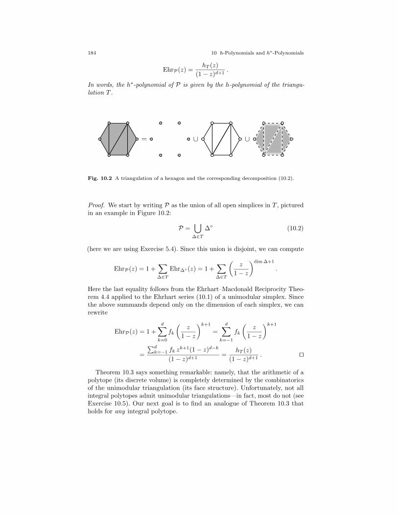
Fig. 10.2 A triangulation of a hexagon and the corresponding decomposition (10.2).

Proof. We start by writing P as the union of all open simplices in T , picturedin an example in Figure 10.2:

P =[

�2T

�� (10.2)

(here we are using Exercise 5.4). Since this union is disjoint, we can compute

EhrP(z) = 1 +X

�2T

Ehr�

�(z) = 1 +X

�2T

✓

z

1� z

◆

dim�+1

.

Here the last equality follows from the Ehrhart–Macdonald Reciprocity Theo-rem 4.4 applied to the Ehrhart series (10.1) of a unimodular simplex. Sincethe above summands depend only on the dimension of each simplex, we canrewrite

EhrP(z) = 1 +d

X

k=0

fk

✓

z

1� z

◆

k+1

=d

X

k=�1

fk

✓

z

1� z

◆

k+1

=

P

d

k=�1

fk

zk+1(1� z)d�k

(1� z)d+1

=hT

(z)

(1� z)d+1

. ut

Theorem 10.3 says something remarkable: namely, that the arithmetic of apolytope (its discrete volume) is completely determined by the combinatoricsof the unimodular triangulation (its face structure). Unfortunately, not allintegral polytopes admit unimodular triangulations—in fact, most do not (seeExercise 10.5). Our next goal is to find an analogue of Theorem 10.3 thatholds for any integral polytope.

10.2 Fundamental Parallelepipeds Open Up, With an h-Twist 185

10.2 Fundamental Parallelepipeds Open Up, With anh-Twist

Our philosophy in constructing a generalization of Theorem 10.3 rests inrevisiting the cone over a given polytope from Chapter 3, using a decompositionof P into open simplices.

Given an integral d-polytope P, fix a (not necessarily unimodular) trian-gulation T . As in (10.2), we can write P as the disjoint union of the opensimplices in T ; from this point of view, the following definition should looknatural. Given a simplex � 2 T , let ⇧(�) be the fundamental parallelepipedof cone(�) (as defined in Section 3.3), and let

B�

(z) := �⇧(�)

�(1, 1, . . . , 1, z) .

Thus B�

(z) is an “open” variant of h⇤�

(z) = �⇧(�)

(1, 1, . . . , 1, z), an equationwe used several times in Chapters 3 and 4.

Looking back at our proof of Theorem 10.3, it makes moral sense to include? in the collection of faces of a triangulation of a given polytope, withthe convention dim(?) := �1. (This explains in hindsight our conventionf�1

:= 1.) We will assume for the rest of this chapter that any triangulation Tincludes the “empty simplex” ?. Along the same lines, we define B?(z) := 1.

We need one more concept to be able to state our generalization of Theorem10.3. Given a simplex � 2 T , let

linkT

(�) := {⌦ 2 T : ⌦ \� = ?, ⌦ ✓ � for some � 2 T with � ✓ �} ,

the link of �. In words, every simplex in linkT

(�) is disjoint from �, yetit is the face of a simplex in T that also contains � as a face; see Figure10.3 for two examples. When the triangulation T is clear from the context,

v

link(v)

l

link(l)

Fig. 10.3 The links of a vertex and an edge in a triangulation of the 3-cube.

we suppress the subscript and simply write link(�). We remark that, bydefinition, link(?) = T . In general, link(�) consists of a collection of simplicesin T , the largest dimension of which is d� dim(�)� 1 (Exercise 10.8), and

186 10 h-Polynomials and h⇤-Polynomials

so it is reasonable to define

hlink(�)

(z) :=

d�dim(�)�1

X

k=�1

fk

zk+1 (1� z)d�dim(�)�1�k ,

where fk

denotes the number of k-simplices in link(�). The h-polynomialof link(�) encodes combinatorial data coming from the simplices in T thatcontain �. This statement can be made more precise, as we invite the readerto prove in Exercise 10.9:

hlink(�)

(z) = (1� z)d�dim(�)

X

�◆�

✓

z

1� z

◆

dim(�)�dim(�)

, (10.3)

where the sum is over all simplices � 2 T containing �.

Theorem 10.4 (Betke–McMullen decomposition of h⇤). Fix a trian-gulation T of the integer d-polytope P. Then

EhrP(z) =

P

�2T

hlink(�)

(z)B�

(z)

(1� z)d+1

.

Before proving Theorem 10.4, we explain its relation to Theorem 10.3.If a simplex � 2 T is unimodular then the corresponding fundamentalparallelepiped ⇧(�) of cone(�) contains the origin as its sole integer latticepoint, and thus B

�

(z) = 0, unless � = ?. Thus, if the triangulation T isunimodular then the sum giving the h⇤-polynomial in Theorem 10.4 collapsesto h

link(?)

(z)B?(z) = hT

(z), and so Theorem 10.3 follows as a special caseof Theorem 10.4.

Proof of Theorem 10.4. We start, as in our proof of Theorem 10.3, by writingP as the disjoint union of all open nonempty simplices in T as in (10.2), andthus, using Ehrhart–Macdonald Reciprocity (Theorem 4.4),

EhrP(z) = 1 +X

�2T\{?}

Ehr�

�(z) = 1 +X

�2T\{?}

(�1)dim(�)+1

h⇤�

�

1

z

�

�

1� 1

z

�

dim�+1

= 1 +

P

�2T\{?} zdim(�)+1(1� z)d�dim(�)h⇤

�

( 1z

)

(1� z)d+1

. (10.4)

Here h⇤�

(z) denotes the h⇤-polynomial of the simplex �. Now we use Exer-cise 10.10:

�⇧(�)

(z) = 1 +X

⌦✓�⌦ 6=?

�⇧(⌦)

�(z) ,

where the sum is over all nonempty faces of �. This identity specializes,choosing z = (1, 1, . . . , 1, z), to

10.3 Palindromic Decompositions of h⇤-Polynomials 187

h⇤�

(z) =X

⌦✓�

B⌦

(z) ,

where now the sum is over all faces of �, including ? (recall that B?(z) = 1).Substituting this back into (10.4) yields

EhrP(z) = 1 +

P

�2T\{?} zdim(�)+1(1� z)d�dim(�)

P

⌦✓�

B⌦

( 1z

)

(1� z)d+1

=

P

�2T

zdim(�)+1(1� z)d�dim(�)

P

⌦✓�

B⌦

( 1z

)

(1� z)d+1

. (10.5)

Recall that the polynomial B�

(z) encodes data about the lattice points inthe interior of the fundamental parallelepiped of cone(�). The symmetryof this parallelepiped gets translated into the palindromy of the associatedpolynomial (Exercise 10.7):

B�

(z) = zdim(�)+1B�

�

1

z

�

. (10.6)

This allows us to rewrite (10.5) further:

h⇤P(z) =

X

�2T

zdim(�)+1(1� z)d�dim(�)

X

⌦✓�

B⌦

✓

1

z

◆

=X

�2T

zdim(�)+1(1� z)d�dim(�)

X

⌦✓�

z� dim(⌦)�1B⌦

(z)

=X

⌦2T

X

�◆⌦

zdim(�)�dim(⌦)(1� z)d�dim(�)B⌦

(z)

=X

⌦2T

(1� z)d�dim(⌦)B⌦

(z)X

�◆⌦

✓

z

1� z

◆

dim(�)�dim(⌦)

.

Theorem 10.4 follows now with (10.3). ut

10.3 Palindromic Decompositions of h⇤-Polynomials

Our next goal is to refine Theorem 10.4 in the case that T comes from aboundary triangulation of P , for which we can exploit Theorem 10.2—rather,its analogue for links, which is the subject of Exercise 10.12. To keep ourexposition accessible, we will only discuss the case that P contains an interiorlattice point; the identities in this and the next section have analogues withoutthis condition, which we will address in the Notes at the end of the chapter.

Theorem 10.5. Suppose P is an integral d-polytope that contains an interiorlattice point. Then there exist unique polynomials a(z) and b(z) such that

188 10 h-Polynomials and h⇤-Polynomials

h⇤P(z) = a(z) + z b(z) ,

a(z) = zd a( 1z

), and b(z) = zd�1 b( 1z

).

The identities for a(z) and b(z) say that a(z) and b(z) are palindromicpolynomials; the degree of a(z) is necessarily d (because the constant coe�cientof a(z) is h⇤

P(0) = 1), while the degree of b(z) is d� 1 or smaller. In fact, b(z)can be the zero polynomial—this happens if and only if P is the translate ofa reflexive polytope, by Theorem 4.6.

Proof. After a harmless lattice translation, we may assume that 0 2 P�. Fixa regular boundary triangulation T of P and let

T0

:= T [ {conv(�,0) : � 2 T} .

Thus T0

is a triangulation of P whose simplices come in two flavors, those onthe boundary of P and those of the form conv(�,0) for some � 2 T . (Wesay that T

0

comes from coning over the boundary triangulation T .) Figure10.4 shows an example. Maybe not surprisingly, the two kinds of simplices in

T0

T

Fig. 10.4 A triangulation T0 and its two types of simplices; the middle picture shows theboundary triangulation T .

T0

are related: Exercise 10.11 says that for any nonempty simplex � 2 T ,

hlink

T0 (�)

(z) = hlink

T0 (conv(�,0))

(z) = hlink

T

(�)

(z) . (10.7)

Thus Theorem 10.4 gives in this case

h⇤P(z) =

X

�2T0

hlink

T0 (�)

(z)B�

(z)

=X

�2T

hlink

T

(�)

(z)�

B�

(z) +Bconv(�,0)

(z)�

.

Now let

10.4 Inequalities for h⇤-Polynomials 189

a(z) :=X

�2T

hlink

T

(�)

(z)B�

(z) (10.8)

b(z) :=1

z

X

�2T

hlink

T

(�)

(z)Bconv(�,0)

(z) . (10.9)

The fact that each Bconv(�,0)

(z) has constant term zero ensures that b(z) isa polynomial (of degree at most d� 1). Furthermore, by Exercise 10.12 and(10.6),

zd a

✓

1

z

◆

=X

�2T

zd�dim(�)�1hlink

T

(�)

✓

1

z

◆

zdim(�)+1B�

✓

1

z

◆

=X

�2T

hlink

T

(�)

(z)B�

(z) = a(z) ,

and b(z) = zd�1 b( 1z

) follows analogously. Thus our setup gives rise to thedecomposition

h⇤P(z) = a(z) + z b(z)

with palindromic polynomials a(z) and b(z), and Exercise 10.13 says thatthis decomposition is unique. (Note that this means, in particular, that anyboundary triangulation yields the same decomposition.) ut

10.4 Inequalities for h⇤-Polynomials

The proof of Theorem 10.5 has a powerful consequence due to the following fact,whose proof would lead us too far astray (though we outline a self-containedproof in Exercises 10.16–10.18).

Theorem 10.6. The h-polynomial of a link in a regular triangulation hasnonnegative coe�cients.

Looking back how the polynomials a(z) and b(z) were constructed (see(10.8) and (10.9)), we can thus deduce:

Corollary 10.7. The polynomials a(z) and b(z) appearing in Theorem 10.5have nonnegative coe�cients.

Naturally, the fact that the coe�cients of a(z) and b(z) have nonnegativecoe�cients can be translated into inequalities among the coe�cients of theaccompanying h⇤-polynomials: the following corollary of Corollary 10.7 iseasily proved (Exercise 10.14).

Corollary 10.8. Suppose P is an integral d-polytope that contains an interiorlattice point. Then its h⇤-polynomial h⇤

P(x) = h⇤d

xd + h⇤d�1

xd�1 + · · · + h⇤0

satisfies

190 10 h-Polynomials and h⇤-Polynomials

h⇤0

+h⇤1

+ · · ·+h⇤j+1

� h⇤d

+h⇤d�1

+ · · ·+h⇤d�j

for 0 j bd

2

c�1 (10.10)

and

h⇤0

+ h⇤1

+ · · ·+ h⇤j

h⇤d

+ h⇤d�1

+ · · ·+ h⇤d�j

for 0 j d. (10.11)

Notes

1. Theorem 10.3 is only one indication how important (and special) unimodulartriangulations are; see [97, Chapter 9] for more. If an integral polytope Padmits a unimodular triangulation, then it is integrally closed: for everypositive integer k and every integer point x 2 kP there exist integer pointsy1

,y2

, . . . ,yk

2 P such that y1

+y2

+· · ·+yk

= x.1 (See Exercise 10.6.) Thereare integrally closed polytopes that do not admit a unimodular triangulation.These two notions are part of an interesting hierarchy of integral polytopes,with connections to commutative algebra and algebraic geometry; see, e.g., [73].

2. Theorem 10.4 is due to Ulrich Betke and Peter McMullen, as is Theorem10.5, published in an influential paper [54] in 1985. Corollary 10.7 shouldhave maybe been in [54] (the nonnegativity of the h-polynomials in Betke–McMullen’s formulas was established in the 1970’s), but it only appeared—inthe guise of Corollary 10.8—in the 1990’s, in papers by Takayuki Hibi [128] andRichard Stanley [221]. Neither paper gives the impression that the inequalitiesof Corollary 10.8 follow immediately from Betke–McMullen’s work, thoughboth hold without the condition of the existence of an interior lattice point(here d has to be replaced by the degree of h⇤

P(z) in (10.11)) and in situationsmore general than the realm of Ehrhart series.

3. Theorem 10.5 and Corollary 10.7 are not the end of the story. Buildingon work of Sam Payne [182] (which gave a multivariate version of Theorem10.4), Alan Stapledon [228] generalized Theorem 10.5 and Corollary 10.7 toarbitrary integral polytopes. His theorem says that, if h⇤

P(z) has degree s(recall from Chapter 4 that in this case we say P has degree s), then thereexist unique polynomials a(z) and b(z) with nonnegative coe�cients such that

�

1 + z + · · ·+ zd�s

�

h⇤P(z) = a(z) + zd+1�s b(z) , (10.12)

a(z) = zd a( 1z

), b(z) = zd�l b( 1z

), and, writing a(z) = ad

zd+ad�1

zd�1+· · ·+a0

,

1 = a0

a1

aj

for 2 j d� 1. (10.13)

1 There is a related notion for integral polytopes, namely that of normality. For full-dimensional polytopes, the adjectives integrally closed and normality are equivalent, butthis is not the case when the subgroup

Px,y2P\Zd

Z(x�y) of Zd is not a direct summand

of Zd. For more about this subtlety (and much more), see [73,87].

Exercises 191

These inequalities imply Corollary 10.8 without the condition that P containsan interior lattice point (again here d has to be replaced by s in (10.11));see Exercise 10.15. Stapledon has recently improved this theorem further,giving infinitely many classes of linear inequalities among the h⇤-coe�cients[226]. This exciting new line of research involves additional techniques fromadditive number theory. He also introduced a weighted variant of the h⇤-polynomial which is always palindromic, motivated by motivic integrationand the cohomology of certain toric varieties [227]. One can easily recover h⇤

P(x)from this weighted h⇤-polynomial, but one can also deduce the palindromy ofboth a(x) and b(x) as coming from the same source (and this perspective hassome serious geometric applications).

Exercises

10.1. | Show that the f -vector and the h-vector of a simplicial d-polytopeare related via

hk

=k

X

j=0

(�1)k�j

✓

d� j

d� k

◆

fj�1

and fk�1

=k

X

j=0

✓

d� j

k � j

◆

hj

,

and conclude that the Dehn–Sommerville relations in Exercise 5.9 are equiva-lent to Theorem 10.1.

10.2. | As in the setup of our proof of Theorem 10.2, let Q ✓ Rd+1 be thelifted polytope giving rise to a regular triangulation T of the polytope P ✓ Rd,choose v 2 P� and lift it to (v, h+ 2) 2 Rd+1, where h is the maximal heightamong the vertices of Q. Let R be the convex hull of (v, h+2) and the verticesof the lower hull of Q, and let

S := R \ �

x 2 Rd+1 : xd+1

= h+ 1

.

Prove that S is a simplicial polytope whose face numbers fk

equal the facenumbers of the triangulation of @P induced by T .

10.3. Given a triangulation T of the boundary of a d-polytope P and a pointv 2 P�, construct a triangulation K of P consisting of T appended by thesimplices conv(�,v) for all � 2 T ; i.e., the new triangulation K comes fromconing over T . Prove that

hK

(z) = hT

(z) .

10.4. | Show that if � is a unimodular k-simplex then

Ehr�

(z) =1

(1� z)k+1

.

192 10 h-Polynomials and h⇤-Polynomials

10.5. Show that any integral polygon admits a unimodular triangulation.Give an example of an integral d-polytope that does not admit a unimodulartriangulation, for any d � 3.

10.6. Recall from the Notes that an integral polytope P is integrally closedif for every positive integer k and every integer point x 2 kP there existinteger points y

1

,y2

, . . . ,yk

2 P such that y1

+y2

+ · · ·+yk

= x. Prove thatany integral polytope that admits a unimodular triangulation is integrallyclosed.

10.7. | Prove (10.6): B�

(z) = zdim(�)+1B�

�

1

z

�

.

10.8. | Let T be a triangulation of the d-polytope P. Given � 2 T , showthat the largest dimension occurring among the simplices in link(�) is d�dim(�)� 1.

10.9. | Prove (10.3): given a triangulation T of a d-dimensional polytope,then for any simplex � 2 T ,

hlink(�)

(z) = (1� z)d�dim(�)

X

�◆�

✓

z

1� z

◆

dim(�)�dim(�)

,

where the sum is over all simplices � 2 T that contain �.

10.10. | For an integral simplex �, let ⇧(�) denote the fundamental paral-lelepiped of cone(�). Show that

�⇧(�)

(z) = 1 +X

⌦✓�

�⇧(⌦)

�(z) ,

where the sum is over all nonempty faces of �.

10.11. | Prove (10.7): Fix a regular triangulation T0

of a polytope Pwith 0 2 P�, whose vertices are 0 and the vertices of P, and let T :={� 2 T

0

: � ✓ @P}. Then for any nonempty � 2 T ,

hlink(�)

(z) = hlink(conv(�,0))

(z) .

10.12. | Let � be a simplex in a regular boundary triangulation of a d-dimensional polytope. Prove that h

link(�)

(z) is palindromic. (Hint: establisha one-to-one correspondence between link(�) and the boundary faces of apolytope of dimension d� dim(�)� 1, respecting the face relations.)

10.13. | Let p(z) be a polynomial of degree d. Show that there are uniquepolynomials a(z) and b(z) such that

p(z) = a(z) + z b(z) ,

a(z) = zd a( 1z

), and b(z) = zd�1 b( 1z

).

Exercises 193

10.14. | Consider the polynomial decomposition h⇤P(z) = a(z) + z b(z) of an

integral d-polytope that contains an interior lattice point, given in Theorem10.5. Prove that the fact that a(z) has nonnegative coe�cients implies (10.10):

h⇤0

+ h⇤1

+ · · ·+ h⇤j+1

� h⇤d

+ h⇤d�1

+ · · ·+ h⇤d�j

for 0 j bd

2

c � 1,

and the fact that b(z) has nonnegative coe�cients implies (10.11):

h⇤0

+ h⇤1

+ · · ·+ h⇤j

h⇤d

+ h⇤d�1

+ · · ·+ h⇤d�j

for 0 j d.

10.15. Derive the analogue of Corollary 10.8 without the condition that Pcontains an interior lattice point, by utilizing (10.12) and (10.13).

10.16. A shelling of the d-polyhedron P is a linear ordering of the facetsF

1

,F2

, . . . ,Fm

of P such that the following recursive conditions hold:

(1) F1

has a shelling.(2) For any j > 1, (F

1

[ F2

[ · · · [ Fj�1

) \ Fj

is of dimension d� 2 and

(F1

[ F2

[ · · · [ Fj�1

) \ Fj

= G1

[ G2

[ · · · [ Gk

,

where G1

[ G2

[ · · · [ Gk

[ · · · [ Gn

is a shelling of Fj

.2

Given a d-polytope P ⇢ Rd, choose a generic vector v 2 Rd (e.g., you canpick a vector at random). If we think of P as a planet and we place a hot airballoon on one of the facets of P, we will slowly see more and more facets,one at a time, as the balloon rises in the direction of v. Here “seeing” meansthe following: we say that a facet F is visible from the point x /2 P if theline segment between x and any point y 2 F intersects P only in y.

Fig. 10.5 Constructing a line shelling of a pentagon.

Our balloon ride gives rise (no pun intended) to an ordering F1

,F2

, . . . ,Fm

of the facets of P. Namely, F1

is the facet we’re starting our journey on, F2

is the next visible facet, etc., until we’re high enough so that no more visible

2 Note that this condition implies that (F1 [ F2 [ · · · [ Fj�1)\F

j

is connected for d � 3.

194 10 h-Polynomials and h⇤-Polynomials

facets can be added. At this point we “pass through infinity” and let theballoon approach the polytope planet from the opposite side. The next facetin our list is the first one that will disappear as we’re moving towards thepolytope, then the next facet that will disappear, etc., until we’re landingback on the polytope. (That is, the second half of our list of facets is thereversed list of what we would get had we started our ride at F

m

.)Prove that this ordering F

1

,F2

, . . . ,Fm

of the facets of P is a shelling(called a line shelling).

10.17. Suppose P is a simplicial d-polytope with facets F1

,F2

, . . . ,Fm

, or-dered by some line shelling. We collect the vertices of F

j

in the set Fj

. LeteFj

be the set of all vertices v 2 Fj

such that Fj

\ {v} is contained in one ofF1

, F2

, . . . , Fj�1

(which define the facets coming earlier in the shelling order).

(a) Prove that the new faces appearing in the jth step of the construction ofthe line shelling, i.e., the faces in F

j

\ (F1

[ F2

[ · · · [ Fj�1

), are precisely

those sets conv(G) for some eFj

✓ G ✓ Fj

.(b) Show that

fk�1

=k

X

m=0

✓

d�m

k �m

◆

ehm

,

where ehm

denotes the number of sets eFj

of cardinality m.

(c) Conclude that ehm

= hm

and thus that hm

� 0.

10.18. Given a regular triangulation of the polytope P, prove that the h-polynomial of the induced triangulation of @P has nonnegative coe�cients,as does the h-polynomial of the link of any simplex in this triangulation.

10.19. Show that the construction in Exercise 10.17 gives the following char-acterization of the h-polynomial of a simple polytope P : fix a generic directionvector v and orient the graph of P so that each oriented edge (viewed as avector) forms an acute angle with v. Then h

k

equals the number of verticesof this oriented graph with in-degree k.

Open Problems

10.20. Which integral polytopes admit a unimodular triangulation? (Theproperty of admitting unimodular triangulations is part of an interestinghierarchy of integral polytopes; see [73].)

10.21. Find a complete set of inequalities for the coe�cients of any h⇤-polynomials of degree 3, i.e., piecewise linear regions in R3 all of whoseinteger points (h⇤

1

, h⇤2

, h⇤3

) come from an h⇤-polynomial of a 3-dimensionalintegral polytope. (See also Open Problem 3.42.)

Open Problems 195

10.22. A linear inequality a0

x0

+a1

x1

+ . . . ad

xd

� 0 is balanced if a0

+a1

+· · ·+ a

d

= 0. Find a complete set of balanced inequalities for the coe�cientsof any h⇤-polynomial of degree 6. (For degree 5, see [226].)

10.23. Prove that every integrally closed reflexive polytope has a unimodalh⇤-polynomial. More generally, prove that every integrally closed polytope hasa unimodal h⇤-polynomial. Even more generally, classify integral polytopeswith a unimodal h⇤-polynomial. (See [12, 63, 74, 204] for possible startingpoints.)