Chapter 9 Model Checking - University of Toronto

Chapter 9

Model Checking

CHAPTER OUTLINE

Section 1 Checking the Sampling ModelSection 2 Checking for Prior–Data ConflictSection 3 The Problem with Multiple Checks

The statistical inference methods developed in Chapters 6 through 8 all depend onvarious assumptions. For example, in Chapter 6 we assumed that the data s weregenerated from a distribution in the statistical model {Pθ : θ ∈ "}. In Chapter 7, wealso assumed that our uncertainty concerning the true value of the model parameter θcould be described by a prior probability distribution#. As such, any inferences drawnare of questionable validity if these assumptions do not make sense in a particularapplication.

In fact, all statistical methodology is based on assumptions or choices made bythe statistical analyst, and these must be checked if we want to feel confident thatour inferences are relevant. We refer to the process of checking these assumptions asmodel checking, the topic of this chapter. Obviously, this is of enormous importancein applications of statistics, and good statistical practice demands that effective modelchecking be carried out. Methods range from fairly informal graphical methods tomore elaborate hypothesis assessment, and we will discuss a number of these.

9.1 Checking the Sampling ModelFrequency-based inference methods start with a statistical model { fθ : θ ∈ "}, for thetrue distribution that generated the data s. This means we are assuming that the truedistribution for the observed data is in this set. If this assumption is not true, thenit seems reasonable to question the relevance of any subsequent inferences we makeabout θ .

Except in relatively rare circumstances, we can never know categorically that amodel is correct. The most we can hope for is that we can assess whether or not theobserved data s could plausibly have arisen from the model.

479

480 Section 9.1: Checking the Sampling Model

If the observed data are surprising for each distribution in the model, then we haveevidence that the model is incorrect. This leads us to think in terms of computing aP-value to check the correctness of the model. Of course, in this situation the nullhypothesis is that the model is correct; the alternative is that the model could be any ofthe other possible models for the type of data we are dealing with.

We recall now our discussion of P-values in Chapter 6, where we distinguishedbetween practical significance and statistical significance. It was noted that, while a P-value may indicate that a null hypothesis is false, in practical terms the deviation fromthe null hypothesis may be so small as to be immaterial for the application. When thesample size gets large, it is inevitable that any reasonable approach via P-values willdetect such a deviation and indicate that the null hypothesis is false. This is also truewhen we are carrying out model checking using P-values. The resolution of this is toestimate, in some fashion, the size of the deviation of the model from correctness, andso determine whether or not the model will be adequate for the application. Even ifwe ultimately accept the use of the model, it is still valuable to know, however, that wehave detected evidence of model incorrectness when this is the case.

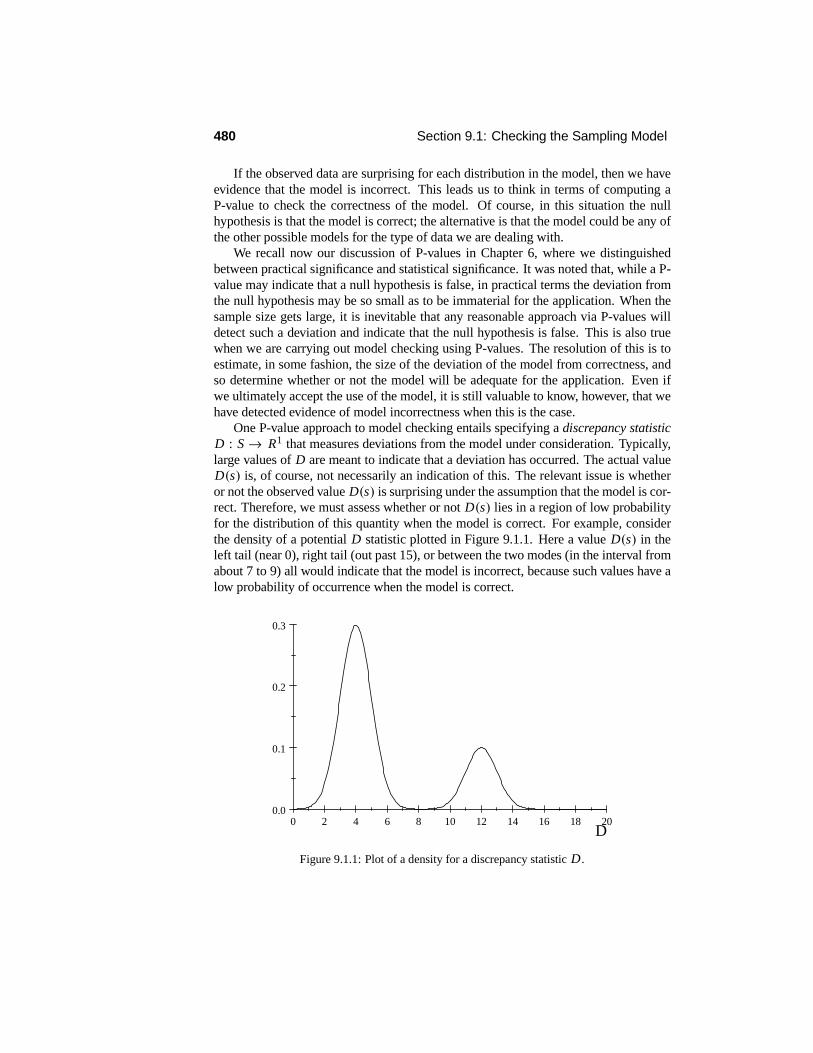
One P-value approach to model checking entails specifying a discrepancy statisticD : S → R1 that measures deviations from the model under consideration. Typically,large values of D are meant to indicate that a deviation has occurred. The actual valueD(s) is, of course, not necessarily an indication of this. The relevant issue is whetheror not the observed value D(s) is surprising under the assumption that the model is cor-rect. Therefore, we must assess whether or not D(s) lies in a region of low probabilityfor the distribution of this quantity when the model is correct. For example, considerthe density of a potential D statistic plotted in Figure 9.1.1. Here a value D(s) in theleft tail (near 0), right tail (out past 15), or between the two modes (in the interval fromabout 7 to 9) all would indicate that the model is incorrect, because such values have alow probability of occurrence when the model is correct.

0 2 4 6 8 10 12 14 16 18 200.0

0.1

0.2

0.3

D

Figure 9.1.1: Plot of a density for a discrepancy statistic D.

Chapter 9: Model Checking 481

The above discussion places the restriction that, when the model is correct, D musthave a single distribution, i.e., the distribution cannot depend on θ . For many com-monly used discrepancy statistics, this distribution is unimodal. A value in the righttail then indicates a lack of fit, or underfitting, by the model (the discrepancies areunnaturally large); a value in the left tail then indicates overfitting by the model (thediscrepancies are unnaturally small).

There are two general methods available for obtaining a single distribution for thecomputation of P-values. One method requires that D be ancillary.

Definition 9.1.1 A statistic D whose distribution under the model does not dependupon θ is called ancillary, i.e., if s ∼ Pθ , then D(s) has the same distribution forevery θ ∈ ".

If D is ancillary, then it has a single distribution specified by the model. If D(s) is asurprising value for this distribution, then we have evidence against the model beingtrue.

It is not the case that any ancillary D will serve as a useful discrepancy statistic.For example, if D is a constant, then it is ancillary, but it is obviously not useful formodel checking. So we have to be careful in choosing D.

Quite often we can find useful ancillary statistics for a model by looking at resid-uals. Loosely speaking, residuals are based on the information in the data that is leftover after we have fit the model. If we have used all the relevant information in the datafor fitting, then the residuals should contain no useful information for inference aboutthe parameter θ . Example 9.1.1 will illustrate more clearly what we mean by residuals.Residuals play a major role in model checking.

The second method works with any discrepancy statistic D. For this, we use theconditional distribution of D, given the value of a sufficient statistic T . By Theorem8.1.2, this conditional distribution is the same for every value of θ . If D(s) is a surpris-ing value for this distribution, then we have evidence against the model being true.

Sometimes the two approaches we have just described agree, but not always. Con-sider some examples.

EXAMPLE 9.1.1 Location NormalSuppose we assume that (x1, . . . , xn) is a sample from an N(µ, σ 2

0) distribution, whereµ ∈ R1 is unknown and σ 2

0 is known. We know that x̄ is a minimal sufficient statisticfor this problem (see Example 6.1.7). Also, x̄ represents the fitting of the model to thedata, as it is the estimate of the unknown parameter value µ.

Now consider

r = r (x1, . . . , xn) = (r1, . . . , rn) = (x1 − x̄, . . . , xn − x̄)

as one possible definition of the residual. Note that we can reconstruct the original datafrom the values of x̄ and r .

It turns out that R = !X1 − X̄, . . . , Xn − X̄"

has a distribution that is independentof µ, with E(Ri ) = 0 and Cov(Ri , R j ) = σ 2

0(δi j − 1/n) for every i, j (δi j = 1 wheni = j and 0 otherwise). Moreover, R is independent of X̄ and Ri ∼ N(0, σ 2

0 (1− 1/n))(see Problems 9.1.19 and 9.1.20).


Accordingly, we have that r is ancillary and so is any discrepancy statistic D thatdepends on the data only through r . Furthermore, the conditional distribution of D(R)given X̄ = x̄ is the same as the marginal distribution of D(R) because they are inde-pendent. Therefore, the two approaches to obtaining a P-value agree here, wheneverthe discrepancy statistic depends on the data only through r.

By Theorem 4.6.6, we have that

D(R) = 1

σ 20

n#i=1

R2i =

1

σ 20

n#i=1

!Xi − X̄

"2is distributed χ2 (n − 1), so this is a possible discrepancy statistic. Therefore, the P-value

P(D > D(r)), (9.1.1)

where D ∼ χ2 (n − 1), provides an assessment of whether or not the model is correct.Note that values of (9.1.1) near 0 or near 1 are both evidence against the model, as

both indicate that D(r) is in a region of low probability when assuming the model iscorrect. A value near 0 indicates that D(r) is in the right tail, whereas a value near 1indicates that D(r) is in the left tail.

The necessity of examining the left tail of the distribution of D(r), as well as theright, is seen as follows. Consider the situation where we are in fact sampling from anN(µ, σ 2) distribution where σ 2 is much smaller than σ 2

0. In this case, we expect D(r)to be a value in the left tail, because E(D(R)) = (n − 1)σ 2/σ 2

0.There are obviously many other choices that could be made for the D statistic.

At present, there is not a theory that prescribes one choice over another. One cautionshould be noted, however. The choice of a statistic D cannot be based upon looking atthe data first. Doing so invalidates the computation of the P-value as described above,as then we must condition on the data feature that led us to choose that particular D.

EXAMPLE 9.1.2 Location-Scale NormalSuppose we assume that (x1, . . . , xn) is a sample from an N(µ, σ 2) distribution, where!µ, σ 2

" ∈ R1 × (0,∞) is unknown. We know that!x̄, s2

"is a minimal sufficient

statistic for this model (Example 6.1.8). Consider

r = r (x1, . . . , xn) = (r1, . . . , rn) =$

x1 − x̄

s, . . . ,

xn − x̄

s

%as one possible definition of the residual. Note that we can reconstruct the data fromthe values of (x̄, s2) and r .

It turns out R has a distribution that is independent of (µ, σ 2) (and hence is an-cillary — see Challenge 9.1.28) as well as independent of (X̄ , S2). So again, the twoapproaches to obtaining a P-value agree here, as long as the discrepancy statistic de-pends on the data only through r.

One possible discrepancy statistic is given by

D(r) = −1n

n#i=1

ln

&r2

i

n − 1

'.


To use this statistic for model checking, we need to obtain its distribution when themodel is correct. Then we compare the observed value D(r) with this distribution, tosee if it is surprising.

We can do this via simulation. Because the distribution of D(R) is independentof (µ, σ 2), we can generate N samples of size n from the N(0, 1) distribution (orany other normal distribution) and calculate D(R) for each sample. Then we lookat histograms of the simulated values to see if D(r), from the original sample, is asurprising value, i.e., if it lies in a region of low probability like a left or right tail.

For example, suppose we observed the sample

−2.08 −0.28 2.01 −1.37 40.08

obtaining the value D(r) = 4.93. Then, simulating 104 values from the distributionof D, under the assumption of model correctness, we obtained the density histogramgiven in Figure 9.1.2. See Appendix B for some code used to carry out this simulation.The value D(r) = 4.93 is out in the right tail and thus indicates that the sample is notfrom a normal distribution. In fact, only 0.0057 of the simulated values are larger, sothis is definite evidence against the model being correct.

7654321

0.8

0.7

0.6

0.5

0.4

0.3

0.2

0.1

0.0

D

den

sity

Figure 9.1.2: A density histogram for a simulation of 104 values of D in Example 9.1.2.

Obviously, there are other possible functions of r that we could use for modelchecking here. In particular, Dskew(r) = (n − 1)−3/2(n

i=1 r3i , the skewness statis-

tic, and Dkurtosis(r) = (n − 1)−2(ni=1 r4

i , the kurtosis statistic, are commonly used.The skewness statistic measures the symmetry in the data, while the kurtosis statisticmeasures the “peakedness” in the data. As just described, we can simulate the distribu-tion of these statistics under the normality assumption and then compare the observedvalues with these distributions to see if we have any evidence against the model (seeComputer Problem 9.1.26).

The following examples present contexts in which the two approaches to computinga P-value for model checking are not the same.


EXAMPLE 9.1.3 Location-Scale CauchySuppose we assume that (x1, . . . , xn) is a sample from the distribution given by µ +σ Z, where Z ∼ t (1) and (µ, σ 2) ∈ R1 × (0,∞) is unknown. This time, (x̄, s2) isnot a minimal sufficient statistic, but the statistic r defined in Example 9.1.2 is stillancillary (Challenge 9.1.28). We can again simulate values from the distribution of R(just generate samples from the t (1) distribution and compute r for each sample) toestimate P-values for any discrepancy statistic such as the D(r) statistics discussed inExample 9.1.2.

EXAMPLE 9.1.4 Fisher’s Exact TestSuppose we take a sample of n from a population of students and observe the values(a1, b1) , . . . , (an, bn) , where ai is gender (A = 1 indicating male, A = 2 indicatingfemale) and bi is a categorical variable for part-time employment status (B = 1 indicat-ing employed, B = 2 indicating unemployed). So each individual is being categorizedinto one of four categories, namely,

Category 1, when A = 1, B = 1,



Category 4, when A = 2, B = 2.

Suppose our model for this situation is that A and B are independent with P(A =1) = α1, P(B = 1) = β1 where α1 ∈ [0, 1] and β1 ∈ [0, 1] are completely unknown.Then letting Xi j denote the count for the category, where A = i, B = j , Example 2.8.5gives that

(X11, X12, X21, X22) ∼ Multinomial(n, α1β1, α1β2, α2β1, α2β2).

As we will see in Chapter 10, this model is equivalent to saying that there is no rela-tionship between gender and employment status.

Denoting the observed cell counts by (x11, x12, x21, x22), the likelihood function isgiven by !

α1β1"x11

!α1β2

"x12!α2β1

"x21!α2β2

"x22

= αx11+x121 (1− α1)

n−x11−x12 βx11+x211

!1− β1

"n−x11−x21

= αx1·1 (1− α1)

n−x1· βx·11

!1− β1

"n−x·1 ,

where (x1·, x·1) = (x11 + x12, x11 + x21). Therefore, the MLE (Problem 9.1.14) isgiven by )

α̂1, β̂1

*=) x1·

n,

x·1n

*.

Note that α̂1 is the proportion of males in the sample and β̂1 is the proportion of allemployed in the sample. Because (x1·, x·1) determines the likelihood function and canbe calculated from the likelihood function, we have that (x1·, x·1) is a minimal sufficientstatistic.


In this example, a natural definition of residual does not seem readily apparent.So we consider looking at the conditional distribution of the data, given the minimalsufficient statistic. The conditional distribution of the sample (A1, B1), . . . , (An, Bn),given the values (x1·, x·1), is the uniform distribution on the set of all samples wherethe restrictions

x11 + x12 = x1·,x11 + x21 = x·1,

x11 + x12 + x21 + x22 = n (9.1.2)

are satisfied. Notice that, given (x1·, x·1), all the other values in (9.1.2) are determinedwhen we specify a value for x11.

It can be shown that the number of such samples is equal to (see Problem 9.1.21)$n

x1·

%$n

x·1

%.

Now the number of samples with prescribed values for x1·, x·1, and x11 = i is given by$n

x1·

%$x1·i

%$n − x1·x·1 − i

%.

Therefore, the conditional probability function of x11, given (x1·, x·1) , is

P(x11 = i | x1·, x·1) =! n

x1·"!x1·

i

"!n−x1·x·1−i

"! nx1·"! n

x·1" =

!x1·i

"!n−x1·x·1−i

"! nx·1" .

This is the Hypergeometric(n, x·1, x1·) probability function.So we have evidence against the model holding whenever x11 is out in the tails of

this distribution. Assessing this requires a tabulation of this distribution or the use of astatistical package with the hypergeometric distribution function built in.

As a simple numerical example, suppose that we took a sample of n = 20 students,obtaining x·1 = 12 unemployed, x1· = 6 males, and x11 = 2 employed males. Thenthe Hypergeometric(20, 12, 6) probability function is given by the following table.

i 0 1 2 3 4 5 6p(i) 0.001 0.017 0.119 0.318 0.358 0.163 0.024

The probability of getting a value as far, or farther, out in the tails than x11 = 2 is equalto the probability of observing a value of x11 with probability of occurrence as smallas or smaller, than x11 = 2. This P-value equals

(0.119+ 0.017+ 0.001)+ 0.024 = 0.161.

Therefore, we have no evidence against the model of independence between A and B.Of course, the sample size is quite small here.


There is another approach here to testing the independence of A and B. In particu-lar, we could only assume the independence of the initial unclassified sample, and thenwe always have

(X11, X12, X21, X22) ∼ Multinomial(n, α11, α12, α21, α22),

where the αi j comprise an unknown probability distribution. Given this model, wecould then test for the independence of A and B.We will discuss this in Section 10.2.

Another approach to model checking proceeds as follows. We enlarge the model toinclude more distributions and then test the null hypothesis that the true model is thesubmodel we initially started with. If we can apply the methods of Section 8.2 to comeup with a uniformly most powerful (UMP) test of this null hypothesis, then we willhave a check of departures from the model of interest — at least as expressed by thepossible alternatives in the enlarged model. If the model passes such a check, however,we are still required to check the validity of the enlarged model. This can be viewed asa technique for generating relevant discrepancy statistics D.

9.1.1 Residual and Probability Plots

There is another, more informal approach to checking model correctness that is oftenused when we have residuals available. These methods involve various plots of theresiduals that should exhibit specific characteristics if the model is correct. While thisapproach lacks the rigor of the P-value approach, it is good at demonstrating grossdeviations from model assumptions. We illustrate this via some examples.

EXAMPLE 9.1.5 Location and Location-Scale Normal ModelsUsing the residuals for the location normal model discussed in Example 9.1.1, we havethat E(Ri ) = 0 and Var(Ri ) = σ 2

0(1− 1/n).We standardize these values so that theyalso have variance 1, and so obtain the standardized residuals (r∗1 , . . . , r∗n ) given by

r∗i =+

n

σ 20 (n − 1)

(xi − x̄). (9.1.3)

The standardized residuals are distributed N(0, 1), and, assuming that n is reasonablylarge, it can be shown that they are approximately independent. Accordingly, we canthink of r∗1 , . . . , r∗n as an approximate sample from the N(0, 1) distribution.

Therefore, a plot of the points!i, r∗i

"should not exhibit any discernible pattern.

Furthermore, all the values in the y-direction should lie in (−3, 3), unless of coursen is very large, in which case we might expect a few values outside this interval. Adiscernible pattern, or several extreme values, can be taken as some evidence that themodel assumption is not correct. Always keep in mind, however, that any observedpattern could have arisen simply from sampling variability when the true model iscorrect. Simulating a few of these residual plots (just generating several samples of nfrom the N(0, 1) distribution and obtaining a residual plot for each sample) will giveus some idea of whether or not the observed pattern is unusual.


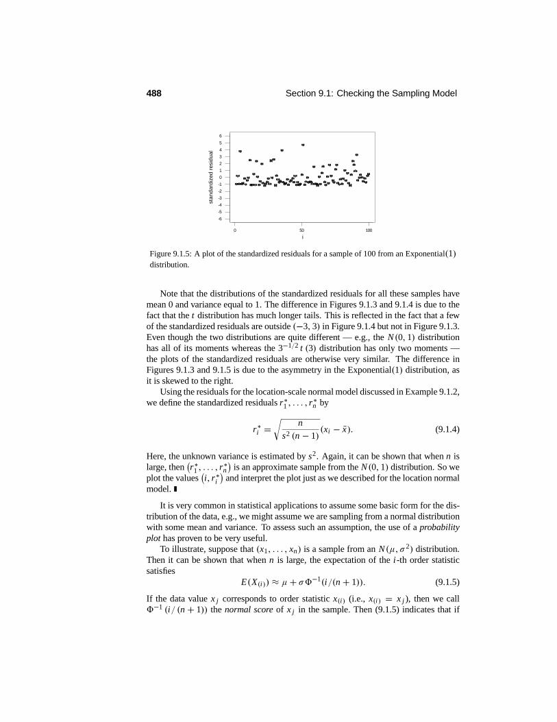
Figure 9.1.3 shows a plot of the standardized residuals (9.1.3) for a sample of 100from the N(0, 1) distribution. Figure 9.1.4 shows a plot of the standardized residualsfor a sample of 100 from the distribution given by 3−1/2 Z, where Z ∼ t (3). Note thata t (3) distribution has mean 0 and variance equal to 3, so Var(3−1/2Z) = 1 (Problem4.6.16). Figure 9.1.5 shows the standardized residuals for a sample of 100 from anExponential(1) distribution.

100500

6

5

4

3

2

1

0

-1

-2

-3

-4

-5

-6

i

stan

dar

diz

ed r

esid

ual

Figure 9.1.3: A plot of the standardized residuals for a sample of 100 from an N(0, 1)distribution.

100500

6

5

4

3

2

1

0

-1

-2

-3

-4

-5

-6

i

stan

dard

ized

res

idua

l

Figure 9.1.4: A plot of the standardized residuals for a sample of 100 from X = 3−1/2Zwhere Z ∼ t(3).


100500

6

5

4

3

2

1

0

-1

-2

-3

-4

-5

-6

i

stan

dard

ized

res

idua

l

Figure 9.1.5: A plot of the standardized residuals for a sample of 100 from an Exponential(1)distribution.

Note that the distributions of the standardized residuals for all these samples havemean 0 and variance equal to 1. The difference in Figures 9.1.3 and 9.1.4 is due to thefact that the t distribution has much longer tails. This is reflected in the fact that a fewof the standardized residuals are outside (−3, 3) in Figure 9.1.4 but not in Figure 9.1.3.Even though the two distributions are quite different — e.g., the N(0, 1) distributionhas all of its moments whereas the 3−1/2 t (3) distribution has only two moments —the plots of the standardized residuals are otherwise very similar. The difference inFigures 9.1.3 and 9.1.5 is due to the asymmetry in the Exponential(1) distribution, asit is skewed to the right.

Using the residuals for the location-scale normal model discussed in Example 9.1.2,we define the standardized residuals r∗1 , . . . , r∗n by

r∗i =,

n

s2 (n − 1)(xi − x̄). (9.1.4)

Here, the unknown variance is estimated by s2. Again, it can be shown that when n islarge, then

!r∗1 , . . . , r∗n

"is an approximate sample from the N(0, 1) distribution. So we

plot the values!i, r∗i

"and interpret the plot just as we described for the location normal

model.

It is very common in statistical applications to assume some basic form for the dis-tribution of the data, e.g., we might assume we are sampling from a normal distributionwith some mean and variance. To assess such an assumption, the use of a probabilityplot has proven to be very useful.

To illustrate, suppose that (x1, . . . , xn) is a sample from an N(µ, σ 2) distribution.Then it can be shown that when n is large, the expectation of the i-th order statisticsatisfies

E(X(i)) ≈ µ+ σ0−1(i/(n + 1)). (9.1.5)

If the data value x j corresponds to order statistic x(i) (i.e., x(i) = x j ), then we call0−1 (i/ (n + 1)) the normal score of x j in the sample. Then (9.1.5) indicates that if


we plot the points (x(i),0−1(i/(n + 1))), these should lie approximately on a linewith intercept µ and slope σ . We call such a plot a normal probability plot or normalquantile plot. Similar plots can be obtained for other distributions.

EXAMPLE 9.1.6 Location-Scale NormalSuppose we want to assess whether or not the following data set can be considered asample of size n = 10 from some normal distribution.

2.00 0.28 0.47 3.33 1.66 8.17 1.18 4.15 6.43 1.77

The order statistics and associated normal scores for this sample are given in the fol-lowing table.

i 1 2 3 4 5x(i) 0.28 0.47 1.18 1.66 1.77

0−1(i/(n + 1)) −1.34 −0.91 −0.61 −0.35 −0.12i 6 7 8 9 10

x(i) 2.00 3.33 4.15 6.43 8.170−1(i/(n + 1)) 0.11 0.34 0.60 0.90 1.33

The values(x(i),0

−1(i/(n + 1)))

are then plotted in Figure 9.1.6. There is some definite deviation from a straight linehere, but note that it is difficult to tell whether this is unexpected in a sample of thissize from a normal distribution. Again, simulating a few samples of the same size (say,from an N(0, 1) distribution) and looking at their normal probability plots is recom-mended. In this case, we conclude that the plot in Figure 9.1.6 looks reasonable.

876543210

1

0

-1

x

Nor

mal

sco

res

Figure 9.1.6: Normal probability plot of the data in Example 9.1.6.

We will see in Chapter 10 that the use of normal probability plots of standardizedresiduals is an important part of model checking for more complicated models. So,while they are not really needed here, we consider some of the characteristics of suchplots when assessing whether or not a sample is from a location normal or location-scale normal model.


Assume that n is large so that we can consider the standardized residuals, givenby (9.1.3) or (9.1.4) as an approximate sample from the N(0, 1) distribution. Then anormal probability plot of the standardized residuals should be approximately linear,with y-intercept approximately equal to 0 and slope approximately equal to 1. If weget a substantial deviation from this, then we have evidence that the assumed model isincorrect.

In Figure 9.1.7, we have plotted a normal probability plot of the standardized resid-uals for a sample of n = 25 from an N(0, 1) distribution. In Figure 9.1.8, we haveplotted a normal probability plot of the standardized residuals for a sample of n = 25from the distribution given by X = 3−1/2 Z, where Z ∼ t (3). Both distributions havemean 0 and variance 1, so the difference in the normal probability plots is due to otherdistributional differences.

210-1-2

2

1

0

-1

-2

Standardized residuals

Nor

mal

sco

res

Figure 9.1.7: Normal probability plot of the standardized residuals of a sample of 25 from anN(0, 1) distribution.

3210-1-2

2

1

0

-1

-2

Standardized residuals

Nor

mal

sco

res

Figure 9.1.8: Normal probability plot of the standardized residuals of a sample of 25 fromX = 3−1/2 Z where Z ∼ t(3) .


9.1.2 The Chi-Squared Goodness of Fit Test

The chi-squared goodness of fit test has an important historical place in any discussionof assessing model correctness. We use this test to assess whether or not a categoricalrandom variable W , which takes its values in the finite sample space {1, 2, . . . , k}, has aspecified probability measure P, after having observed a sample (w1, . . . ,wn). Whenwe have a random variable that is discrete and takes infinitely many values, then wepartition the possible values into k categories and let W simply indicate which categoryhas occurred. If we have a random variable that is quantitative, then we partition R1

into k subintervals and let W indicate in which interval the response occurred. In effect,we want to check whether or not a specific probability model, as given by P, is correctfor W based on an observed sample.

Let (X1, . . . , Xk) be the observed counts or frequencies of 1, . . . , k, respectively.If P is correct, then, from Example 2.8.5,

(X1, . . . , Xk) ∼ Multinomial(n, p1, . . . , pk)

where pi = P({i}). This implies that E(Xi) = npi and Var(Xi) = npi (1− pi ) (recallthat Xi ∼ Binomial(n, pi )). From this, we deduce that

Ri = Xi − npi√npi (1− pi )

D→ N(0, 1) (9.1.6)

as n →∞ (see Example 4.4.9).For finite n, the distribution of Ri , when the model is correct, is dependent on

P, but the limiting distribution is not. Thus we can think of the Ri as standardizedresiduals when n is large. Therefore, it would seem that a reasonable discrepancystatistic is given by the sum of the squares of the standardized residuals with

(ki=1 R2

iapproximately distributed χ2 (k) . The restriction x1+· · ·+ xk = n holds, however, sothe Ri are not independent and the limiting distribution is not χ2(k). We do, however,have the following result, which provides a similar discrepancy statistic.

Theorem 9.1.1 If (X1, . . . , Xk) ∼Multinomial(n, p1, . . . , pk), then

X2 =k#

i=1

(1− pi ) R2i =

k#i=1

(Xi − npi )2

npi

D→ χ2 (k − 1)

as n →∞.The proof of this result is a little too involved for this text, so see, for example, Theorem17.2 of Asymptotic Statistics by A. W. van der Vaart (Cambridge University Press,Cambridge, 1998), which we will use here.

We refer to X2 as the chi-squared statistic. The process of assessing the correctnessof the model by computing the P-value P(X2 ≥ X2

0), where X2 ∼ χ2 (k − 1) andX2

0 is the observed value of the chi-squared statistic, is referred to as the chi-squaredgoodness of fit test. Small P-values near 0 provide evidence of the incorrectness of theprobability model. Small P-values indicate that some of the residuals are too large.


Note that the i th term of the chi-squared statistic can be written as

(Xi − npi )2

npi= (number in the i th cell − expected number in the i th cell)2

expected number in the i th cell.

It is recommended, for example, in Statistical Methods, by G. Snedecor and W. Cochran(Iowa State Press, 6th ed., Ames, 1967) that grouping (combining cells) be employed toensure that E(Xi ) = npi ≥ 1 for every i, as simulations have shown that this improvesthe accuracy of the approximation to the P-value.

We consider an important application.

EXAMPLE 9.1.7 Testing the Accuracy of a Random Number GeneratorIn effect, every Monte Carlo simulation can be considered to be a set of mathematicaloperations applied to a stream of numbers U1,U2, . . . in [0, 1] that are supposed tobe i.i.d. Uniform[0, 1]. Of course, they cannot satisfy this requirement exactly becausethey are generated according to some deterministic function. Typically, a functionf : [0, 1]m → [0, 1] is chosen and is applied iteratively to obtain the sequence. So weselect U1, . . . ,Um as initial seed values and then Um+1 = f (U1, . . . ,Um) ,Um+2 =f (U2, . . . ,Um+1) , etc. There are many possibilities for f, and a great deal of re-search and study have gone into selecting functions that will produce sequences thatadequately mimic the properties of an i.i.d. Uniform[0, 1] sequence.

Of course, it is always possible that the underlying f used in a particular statisticalpackage or other piece of software is very poor. In such a case, the results of thesimulations can be grossly in error. How do we assess whether a particular f is goodor not? One approach is to run a battery of statistical tests to see whether the sequenceis behaving as we know an ideal sequence would.

For example, if the sequence U1,U2, . . . is i.i.d. Uniform[0, 1], then

310U14, 310U24, . . .is i.i.d. Uniform{1, 2, . . . , 10} (3x4 denotes the smallest integer greater than x, e.g.,33.24 = 4). So we can test the adequacy of the underlying function f by generatingU1, . . . ,Un for large n, putting xi = 310Ui4, and then carrying out a chi-squaredgoodness of fit test with the 10 categories {1, . . . , 10} with each cell probability equalto 1/10.

Doing this using a popular statistical package (with n = 104) gave the followingtable of counts xi and standardized residuals ri as specified in (9.1.6).

i xi ri

1 993 −0.233332 1044 1.466673 1061 2.033334 1021 0.700005 1017 0.566676 973 −0.900007 975 −0.833338 965 −1.166679 996 −0.13333

10 955 −1.50000


All the standardized residuals look reasonable as possible values from an N(0, 1) dis-tribution. Furthermore,

X20 = (1− 0.1)

(−0.23333)2 + (1.46667)2 + (2.03333)2

+ (0.70000)2 + (0.56667)2 + (−0.90000)2

+ (−0.83333)2 + (−1.16667)2 + (−0.13333)2

+ (−1.50000)2

= 11.0560

gives the P-value P(X2 ≥ 11.0560) = 0.27190 when X2 ∼ χ2(9). This indicates thatwe have no evidence that the random number generator is defective.

Of course, the story does not end with a single test like this. Many other featuresof the sequence should be tested. For example, we might want to investigate the inde-pendence properties of the sequence and so test if each possible combination of (i, j)occurs with probability 1/100, etc.

More generally, we will not have a prescribed probability distribution P for X butrather a statistical model {Pθ : θ ∈ "}, where each Pθ is a probability measure on thefinite set {1, 2, . . . , k}. Then, based on the sample from the model, we have that

(X1, . . . , Xk) ∼ Multinomial(n, p1(θ), . . . , pk(θ))

where pi (θ) = Pθ ({i}).Perhaps a natural way to assess whether or not this model fits the data is to find the

MLE θ̂ from the likelihood function

L(θ | x1, . . . , xk) = (p1(θ))x1 · · · (pk(θ))

xk

and then look at the standardized residuals

ri (θ̂) = xi − npi (θ̂)4npi (θ̂)(1− pi(θ̂))

.

We have the following result, which we state without proof.

Theorem 9.1.2 Under conditions (similar to those discussed in Section 6.5), we

have that Ri (θ̂)D→ N(0, 1) and

X2 =k#

i=1

(1− pi(θ̂))R2i (θ̂) =

k#i=1

(Xi − npi (θ̂))2

npi(θ̂)

D→ χ2 (k − 1− dim")

as n →∞.By dim", we mean the dimension of the set ". Loosely speaking, this is the mini-mum number of coordinates required to specify a point in the set, e.g., a line requiresone coordinate (positive or negative distance from a fixed point), a circle requires onecoordinate, a plane in R3 requires two coordinates, etc. Of course, this result impliesthat the number of cells must satisfy k > 1+ dim".


Consider an example.

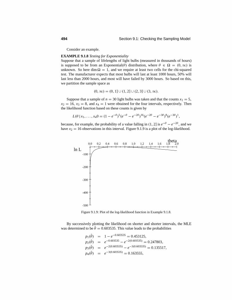
EXAMPLE 9.1.8 Testing for ExponentialitySuppose that a sample of lifelengths of light bulbs (measured in thousands of hours)is supposed to be from an Exponential(θ) distribution, where θ ∈ " = (0,∞) isunknown. So here dim" = 1, and we require at least two cells for the chi-squaredtest. The manufacturer expects that most bulbs will last at least 1000 hours, 50% willlast less than 2000 hours, and most will have failed by 3000 hours. So based on this,we partition the sample space as

(0,∞) = (0, 1] ∪ (1, 2] ∪ (2, 3] ∪ (3,∞).Suppose that a sample of n = 30 light bulbs was taken and that the counts x1 = 5,

x2 = 16, x3 = 8, and x4 = 1 were obtained for the four intervals, respectively. Thenthe likelihood function based on these counts is given by

L(θ | x1, . . . , x40 = (1− e−θ )5(e−θ − e−2θ )16(e−2θ − e−3θ )8(e−3θ )1,

because, for example, the probability of a value falling in (1, 2] is e−θ − e−2θ , and wehave x2 = 16 observations in this interval. Figure 9.1.9 is a plot of the log-likelihood.

0.0 0.2 0.4 0.6 0.8 1.0 1.2 1.4 1.6 1.8 2.0

-500

-400

-300

-200

-100

theta

ln L

Figure 9.1.9: Plot of the log-likelihood function in Example 9.1.8.

By successively plotting the likelihood on shorter and shorter intervals, the MLEwas determined to be θ̂ = 0.603535. This value leads to the probabilities

p1(θ̂) = 1− e−0.603535 = 0.453125,

p2(θ̂) = e−0.603535 − e−2(0.603535) = 0.247803,

p3(θ̂) = e−2(0.603535) − e−3(0.603535) = 0.135517,

p4(θ̂) = e−3(0.603535) = 0.163555,


the fitted values

30p1(θ̂) = 13.59375,

30p2(θ̂) = 7.43409,

30p3(θ̂) = 4.06551,

30p4(θ̂) = 4.90665,

and the standardized residuals

r1(θ̂) = (5− 13.59375) /5

30 (0.453125) (1− 0.453125) = −3.151875,

r2(θ̂) = (16− 7.43409) /5

30 (0.247803) (1− 0.247803) = 3.622378,

r3(θ̂) = (8− 4.06551) /5

30 (0.135517) (1− 0.135517) = 2.098711,

r4(θ̂) = (1− 4.90665) /5

30 (0.163555) (1− 0.163555) = −1.928382.

Note that two of the standardized residuals look large. Finally, we compute

X20 = (1− 0.453125) (−3.151875)2 + (1− 0.247803) (3.622378)2

+ (1− 0.135517) (2.098711)2 + (1− 0.163555) (−1.928382)2

= 22.221018

andP)

X2 ≥ 22.221018*= 0.0000

when X2 ∼ χ2 (2) . Therefore, we have strong evidence that the Exponential(θ)modelis not correct for these data and we would not use this model to make inference aboutθ .

Note that we used the MLE of θ based on the count data and not the original sample!If instead we were to use the MLE for θ based on the original sample (in this case, equalto x̄ and so much easier to compute), then Theorem 9.1.2 would no longer be valid.

The chi-squared goodness of fit test is but one of many discrepancy statistics thathave been proposed for model checking in the statistical literature. The general ap-proach is to select a discrepancy statistic D, like X2, such that the exact or asymptoticdistribution of D is independent of θ and known. We then compute a P-value based onD. The Kolmogorov–Smirnov test and the Cramer–von Mises test are further examplesof such discrepancy statistics, but we do not discuss these here.

9.1.3 Prediction and Cross-Validation

Perhaps the most rigorous test that a scientific model or theory can be subjected tois assessing how well it predicts new data after it has been fit to an independent dataset. In fact, this is a crucial step in the acceptance of any new empirically developedscientific theory — to be accepted, it must predict new results beyond the data that ledto its formulation.

If a model does not do a good job at predicting new data, then it is reasonable to saythat we have evidence against the model being correct. If the model is too simple, then


the fitted model will underfit the observed data and also the future data. If the model istoo complicated, then the model will overfit the original data, and this will be detectedwhen we consider the new data in light of this fitted model.

In statistical applications, we typically cannot wait until new data are generated tocheck the model. So statisticians use a technique called cross-validation. For this, wesplit an original data set x1, . . . , xn into two parts: the training set T, comprising k ofthe data values and used to fit the model; and the validation set V , which comprisesthe remaining n− k data values. Based on the training data, we construct predictors ofvarious aspects of the validation data. Using the discrepancies between the predictedand actual values, we then assess whether or not the validation set V is surprising as apossible future sample from the model.

Of course, there are $n

k

%possible such splits of the data and we would not want to make a decision based onjust one of these. So a cross-validational analysis will have to take this into account.Furthermore, we will have to decide how to measure the discrepancies between T andV and choose a value for k.We do not pursue this topic any further in this text.

9.1.4 What Do We Do When a Model Fails?

So far we have been concerned with determining whether or not an assumed model isappropriate given observed data. Suppose the result of our model checking is that wedecide a particular model is inappropriate. What do we do now?

Perhaps the obvious response is to say that we have to come up with a more appro-priate model — one that will pass our model checking. It is not obvious how we shouldgo about this, but statisticians have devised some techniques.

One of the simplest techniques is the method of transformations. For example, sup-pose that we observe a sample y1, . . . , yn from the distribution given by Y = exp(X)with X ∼ N(µ, σ 2). A normal probability plot based on the yi , as in Figure 9.1.10,will detect evidence of the nonnormality of the distribution. Transforming these yivalues to ln yi will, however, yield a reasonable looking normal probability plot, as inFigure 9.1.11.

So in this case, a simple transformation of the sample yields a data set that passesthis check. In fact, this is something statisticians commonly do. Several transforma-tions from the family of power transformations given by Y p for p 6= 0, or the logarithmtransformation ln Y, are tried to see if a distributional assumption can be satisfied by atransformed sample. We will see some applications of this in Chapter 10. Surprisingly,this simple technique often works, although there are no guarantees that it always will.

Perhaps the most commonly applied transformation is the logarithm when our datavalues are positive (note that this is a necessity for this transformation). Another verycommon transformation is the square root transformation, i.e., p = 1/2,when we havecount data. Of course, it is not correct to try many, many transformations until we findone that makes the probability plots or residual plots look acceptable. Rather, we try afew simple transformations.


6543210

2

1

0

-1

-2

Y

Nor

mal

sco

res

Figure 9.1.10: A normal probability plot of a sample of n = 50 from the distribution given byY = exp(X) with X ∼ N(0, 1).

210-1-2-3

2

1

0

-1

-2

Y

Nor

mal

sco

res

Figure 9.1.11: A normal probability plot of a sample of n = 50 from the distribution given byln Y , where Y = exp(X) and X ∼ N (0, 1).

Summary of Section 9.1

• Model checking is a key component of the practical application of statistics.

• One approach to model checking involves choosing a discrepancy statistic D andthen assessing whether or not the observed value of D is surprising by computinga P-value.


• Computation of the P-value requires that the distribution of D be known underthe assumption that the model is correct. There are two approaches to accom-plishing this. One involves choosing D to be ancillary, and the other involvescomputing the P-value using the conditional distribution of the data given theminimal sufficient statistic.

• The chi-squared goodness of fit statistic is a commonly used discrepancy statis-tic. For large samples, with the expected cell counts determined by the MLEbased on the multinomial likelihood, the chi-squared goodness of fit statistic isapproximately ancillary.

• There are also many informal methods of model checking based on various plotsof residuals.

• If a model is rejected, then there are several techniques for modifying the model.These typically involve transformations of the data. Also, a model that fails amodel-checking procedure may still be useful, if the deviation from correctnessis small.

EXERCISES

9.1.1 Suppose the following sample is assumed to be from an N(θ, 4) distribution withθ ∈ R1 unknown.

1.8 2.1 −3.8 −1.7 −1.3 1.1 1.0 0.0 3.3 1.0−0.4 −0.1 2.3 −1.6 1.1 −1.3 3.3 −4.9 −1.1 1.9

Check this model using the discrepancy statistic of Example 9.1.1.9.1.2 Suppose the following sample is assumed to be from an N(θ, 2) distribution withθ unknown.

−0.4 1.9 −0.3 −0.2 0.0 0.0 −0.1 −1.1 2.0 0.4

(a) Plot the standardized residuals.(b) Construct a normal probability plot of the standardized residuals.(c) What conclusions do you draw based on the results of parts (a) and (b)?9.1.3 Suppose the following sample is assumed to be from an N(µ, σ 2) distribution,where µ ∈ R1 and σ 2 > 0 are unknown.

14.0 9.4 12.1 13.4 6.3 8.5 7.1 12.4 13.3 9.1

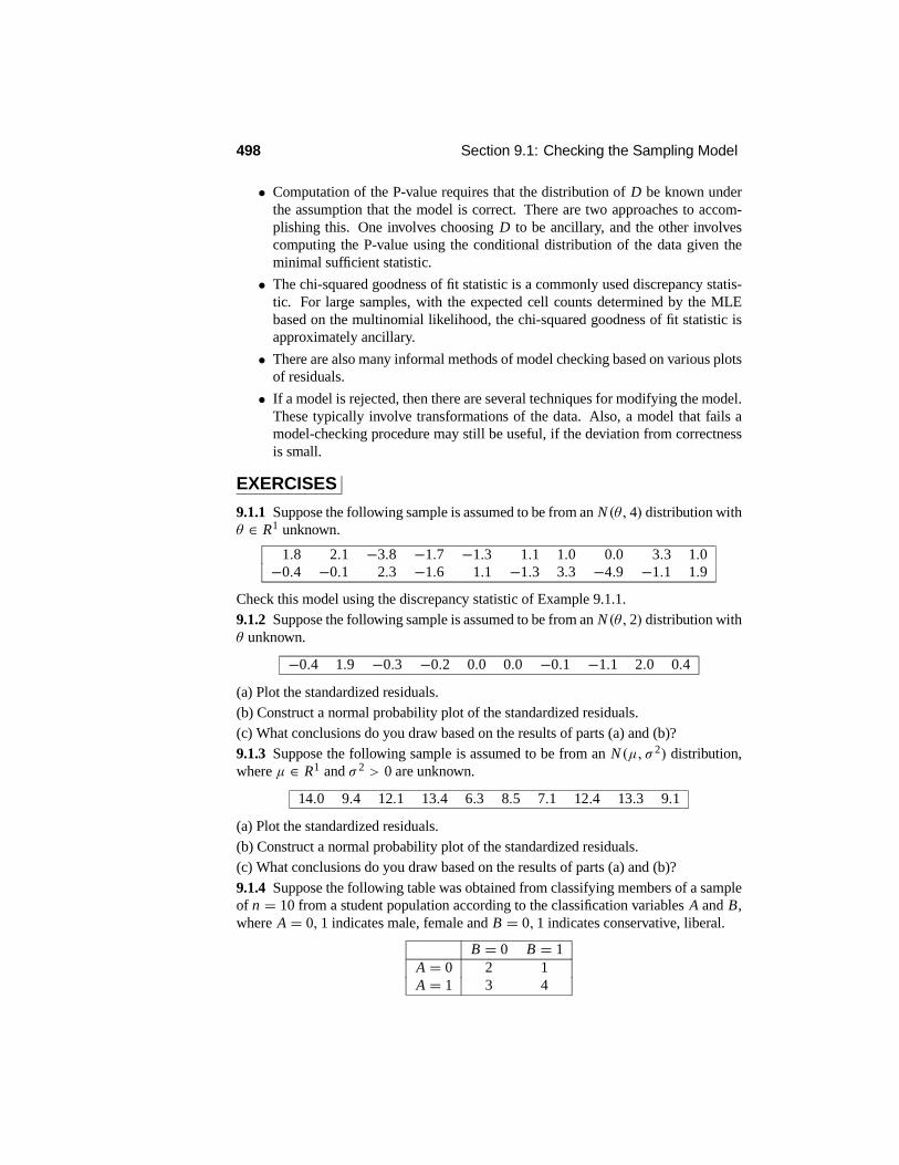
(a) Plot the standardized residuals.(b) Construct a normal probability plot of the standardized residuals.(c) What conclusions do you draw based on the results of parts (a) and (b)?9.1.4 Suppose the following table was obtained from classifying members of a sampleof n = 10 from a student population according to the classification variables A and B,where A = 0, 1 indicates male, female and B = 0, 1 indicates conservative, liberal.

B = 0 B = 1A = 0 2 1A = 1 3 4


Check the model that says gender and political orientation are independent, usingFisher’s exact test.9.1.5 The following sample of n = 20 is supposed to be from a Uniform[0, 1] distrib-ution.

0.11 0.56 0.72 0.18 0.26 0.32 0.42 0.22 0.96 0.040.45 0.22 0.08 0.65 0.32 0.88 0.76 0.32 0.21 0.80

After grouping the data, using a partition of five equal-length intervals, carry out thechi-squared goodness of fit test to assess whether or not we have evidence against thisassumption. Record the standardized residuals.9.1.6 Suppose a die is tossed 1000 times, and the following frequencies are obtainedfor the number of pips up when the die comes to a rest.

x1 x2 x3 x4 x5 x6163 178 142 150 183 184

Using the chi-squared goodness of fit test, assess whether we have evidence that this isnot a symmetrical die. Record the standardized residuals.9.1.7 Suppose the sample space for a response is given by S = {0, 1, 2, 3, . . .}.(a) Suppose that a statistician believes that in fact the response will lie in the set S ={10, 11, 12, 13, . . .} and so chooses a probability measure P that reflects this. Whenthe data are collected, however, the value s = 3 is observed. What is an appropriateP-value to quote as a measure of how surprising this value is as a potential value fromP?(b) Suppose instead P is taken to be a Geometric(0.1) distribution. Determine an ap-propriate P-value to quote as a measure of how surprising s = 3 is as a potential valuefrom P .

9.1.8 Suppose we observe s = 3 heads in n = 10 independent tosses of a purportedlyfair coin. Compute a P-value that assesses how surprising this value is as a potentialvalue from the distribution prescribed. Do not use the chi-squared test.9.1.9 Suppose you check a model by computing a P-value based on some discrepancystatistic and conclude that there is no evidence against the model. Does this mean themodel is correct? Explain your answer.9.1.10 Suppose you are told that standardized scores on a test are distributed N(0, 1).A student’s standardized score is−4. Compute an appropriate P-value to assess whetheror not the statement is correct.9.1.11 It is asserted that a coin is being tossed in independent tosses. You are somewhatskeptical about the independence of the tosses because you know that some peoplepractice tossing coins so that they can increase the frequency of getting a head. So youwish to assess the independence of (x1, . . . , xn) from a Bernoulli(θ) distribution.(a) Show that the conditional distribution of (x1, . . . , xn) given x̄ is uniform on the setof all sequences of length n with entries from {0, 1}.(b) Using this conditional distribution, determine the distribution of the number of 1’sobserved in the first 8n/29 observations. (Hint: The hypergeometric distribution.)


(c) Suppose you observe (1, 1, 1, 1, 1, 0, 0, 0, 0, 1). Compute an appropriate P-value toassess the independence of these tosses using (b).

COMPUTER EXERCISES

9.1.12 For the data of Exercise 9.1.1, present a normal probability plot of the standard-ized residuals and comment on it.9.1.13 Generate 25 samples from the N(0, 1) distribution with n = 10 and look attheir normal probability plots. Draw any general conclusions.9.1.14 Suppose the following table was obtained from classifying members of a sam-ple on n = 100 from a student population according to the classification variables Aand B, where A = 0, 1 indicates male, female and B = 0, 1 indicates conservative,liberal.

B = 0 B = 1A = 0 20 15A = 1 36 29

Check the model that gender and political orientation are independent using Fisher’sexact test.9.1.15 Using software, generate a sample of n = 1000 from the Binomial(10, 0.2)distribution. Then, using the chi-squared goodness of fit test, check that this sample isindeed from this distribution. Use grouping to ensure E(Xi ) = npi ≥ 1. What wouldyou conclude if you got a P-value close to 0?9.1.16 Using a statistical package, generate a sample of n = 1000 from the Poisson(5)distribution. Then, using the chi-squared goodness of fit test based on grouping theobservations into five cells chosen to ensure E(Xi ) = npi ≥ 1, check that this sampleis indeed from this distribution. What would you conclude if you got a P-value closeto 0?9.1.17 Using a statistical package, generate a sample of n = 1000 from the N (0, 1)distribution. Then, using the chi-squared goodness of fit test based on grouping theobservations into five cells chosen to ensure E(Xi ) = npi ≥ 1, check that this sampleis indeed from this distribution. What would you conclude if you got a P-value closeto 0?

PROBLEMS

9.1.18 (Multivariate normal distribution) A random vector Y = (Y1, . . . , Yk) is said tohave a multivariate normal distribution with mean vector µ ∈ Rk and variance matrix2 = (σ i j) ∈ Rk×k if

a1Y1 + · · · + akYk ∼ N

&k#

i=1

aiµi ,k#

i=1

k#j=1

ai a jσ i j

'

for every choice of a1, . . . , ak ∈ R1. We write Y ∼ Nk(µ,2). Prove that E(Yi ) = µi ,Cov(Yi ,Y j) = σ i j and that Yi ∼ N(µi , σ ii ). (Hint: Theorem 3.3.4.)


9.1.19 In Example 9.1.1, prove that the residual R = (R1, . . . , Rn) is distributed mul-tivariate normal (see Problem 9.1.18) with mean vector µ = (0, . . . , 0) and variancematrix 2 = (σ i j) ∈ Rk×k , where σ i j = −σ 2

0/n when i 6= j and σ i i = σ 20(1− 1/n).

(Hint: Theorem 4.6.1.)9.1.20 If Y = (Y1, . . . ,Yk) is distributed multivariate normal with mean vectorµ ∈ Rk

and variance matrix 2 = (σ i j ) ∈ Rk×k, and if X = (X1, . . . , Xl) is distributed multi-variate normal with mean vector ν ∈ Rl and variance matrix ϒ = (τ i j ) ∈ Rl×l , then itcan be shown that Y and X are independent whenever

(ki=1 ai Yi and

(li=1 bi Xi are

independent for every choice of (a1, . . . , ak) and (b1, . . . , bl). Use this fact to showthat, in Example 9.1.1, X̄ and R are independent. (Hint: Theorem 4.6.2 and Problem9.1.19.)9.1.21 In Example 9.1.4, prove that (α̂1, β̂1) = (x1·/n, x·1/n) is the MLE.

9.1.22 In Example 9.1.4, prove that the number of samples satisfying the constraints(9.1.2) equals $

n

x1·

%$n

x·1

%.

(Hint: Using i for the count x11, show that the number of such samples equals$n

x1·

% min{x1·,x·1}#i=max{0,x1·+x·1−n}

$x1·i

%$n − x1·x·1 − i

%and sum this using the fact that the sum of Hypergeometric(n, x·1, x1·) probabilitiesequals 1.)

COMPUTER PROBLEMS

9.1.23 For the data of Exercise 9.1.3, carry out a simulation to estimate the P-value forthe discrepancy statistic of Example 9.1.2. Plot a density histogram of the simulatedvalues. (Hint: See Appendix B for appropriate code.)9.1.24 When n = 10, generate 104 values of the discrepancy statistic in Example 9.1.2when we have a sample from an N(0, 1) distribution. Plot these in a density histogram.Repeat this, but now generate from a Cauchy distribution. Compare the histograms (donot forget to make sure both plots have the same scales).9.1.25 The following data are supposed to have come from an Exponential(θ) distrib-ution, where θ > 0 is unknown.

1.5 1.6 1.4 9.7 12.1 2.7 2.2 1.6 6.8 0.10.8 1.7 8.0 0.2 12.3 2.2 0.2 0.6 10.1 4.9

Check this model using a chi-squared goodness of fit test based on the intervals

(−∞, 2.0], (2.0, 4.0], (4.0, 6.0], (6.0, 8.0], (8.0, 10.0], (10.0,∞).(Hint: Calculate the MLE by plotting the log-likelihood over successively smaller in-tervals.)

502 Section 9.2: Checking for Prior–Data Conflict

9.1.26 The following table, taken from Introduction to the Practice of Statistics, by D.Moore and G. McCabe (W. H. Freeman, New York, 1999), gives the measurements inmilligrams of daily calcium intake for 38 women between the ages of 18 and 24 years.

808 882 1062 970 909 802 374 416 784 997651 716 438 1420 1425 948 1050 976 572 403626 774 1253 549 1325 446 465 1269 671 696

1156 684 1933 748 1203 2433 1255 110

(a) Suppose that the model specifies a location normal model for these data with σ 20 =

(500)2. Carry out a chi-squared goodness of fit test on these data using the intervals(−∞, 600], (600, 1200], (1200, 1800], (1800,∞). (Hint: Plot the log-likelihood oversuccessively smaller intervals to determine the MLE to about one decimal place. Todetermine the initial range for plotting, use the overall MLE of µminus three standarderrors to the overall MLE plus three standard errors.)(b) Compare the MLE of µ obtained in part (a) with the ungrouped MLE.(c) It would be more realistic to assume that the variance σ 2 is unknown as well. Recordthe log-likelihood for the grouped data. (More sophisticated numerical methods areneeded to find the MLE of

!µ, σ 2

"in this case.)

9.1.27 Generate 104 values of the discrepancy statistics Dskew and Dkurtosis in Example9.1.2 when we have a sample of n = 10 from an N(0, 1) distribution. Plot thesein density histograms. Indicate how you would use these histograms to assess thenormality assumption when we had an actual sample of size 10. Repeat this for n = 20and compare the distributions.

CHALLENGES

9.1.28 (MV) Prove that when (x1, . . . , xn) is a sample from the distribution given byµ + σ Z , where Z has a known distribution and (µ, σ 2) ∈ R1 × (0,∞) is unknown,then the statistic

r(x1, . . . , xn) =$

x1 − x̄

s, . . . ,

xn − x̄

s

%is ancillary. (Hint: Write a sample element as xi = µ + σ zi and then show thatr(x1, . . . , xn) can be written as a function of the zi .)

9.2 Checking for Prior–Data ConflictBayesian methodology adds the prior probability measure # to the statistical model{Pθ : θ ∈ "}, for the subsequent statistical analysis. The methods of Section 9.1 aredesigned to check that the observed data can realistically be assumed to have comefrom a distribution in {Pθ : θ ∈ "}. When we add the prior, we are in effect sayingthat our knowledge about the true distribution leads us to assign the prior predictiveprobability M, given by M(A) = E#(Pθ (A)) for A ⊂ ", to describe the processgenerating the data. So it would seem, then, that a sensible Bayesian model-checking


approach would be to compare the observed data s with the distribution given by M,to see if it is surprising or not.

Suppose that we were to conclude that the Bayesian model was incorrect afterdeciding that s is a surprising value from M. This only tells us, however, that theprobability measure M is unlikely to have produced the data and not that the model{Pθ : θ ∈ "} was wrong. Consider the following example.

EXAMPLE 9.2.1 Prior–Data ConflictSuppose we obtain a sample consisting of n = 20 values of s = 1 from the model with" = {1, 2} and probability functions for the basic response given by the followingtable.

s = 0 s = 1f1 (s) 0.9 0.1f2 (s) 0.1 0.9

Then the probability of obtaining this sample from f2 is given by (0.9)20 = 0.12158,which is a reasonable value, so we have no evidence against the model { f1, f2}.

Suppose we place a prior on " given by#({1}) = 0.9999, so that we are virtuallycertain that θ = 1. Then the probability of getting these data from the prior predictiveM is

(0.9999) (0.1)20 + (0.0001) (0.9)20 = 1.2158× 10−5.

The prior probability of observing a sample of 20, whose prior predictive probability isno greater than 1.2158× 10−5, can be calculated (using statistical software to tabulatethe prior predictive) to be approximately 0.04. This tells us that the observed data are“in the tails” of the prior predictive and thus are surprising, which leads us to concludethat we have evidence that M is incorrect.

So in this example, checking the model { fθ : θ ∈ "} leads us to conclude that it isplausible for the data observed. On the other hand, checking the model given by Mleads us to the conclusion that the Bayesian model is implausible.

The lesson of Example 9.2.1 is that we can have model failure in the Bayesian con-text in two ways. First, the data s may be surprising in light of the model { fθ : θ ∈ "}.Second, even when the data are plausibly from this model, the prior and the data mayconflict. This conflict will occur whenever the prior assigns most of its probability todistributions in the model for which the data are surprising. In either situation, infer-ences drawn from the Bayesian model may be flawed.

If, however, the prior assigns positive probability (or density) to every possiblevalue of θ, then the consistency results for Bayesian inference mentioned in Chapter 7indicate that a large amount of data will overcome a prior–data conflict (see Example9.2.4). This is because the effect of the prior decreases with increasing amounts of data.So the existence of a prior–data conflict does not necessarily mean that our inferencesare in error. Still, it is useful to know whether or not this conflict exists, as it is oftendifficult to detect whether or not we have sufficient data to avoid the problem.

Therefore, we should first use the checks discussed in Section 9.1 to ensure that thedata s is plausibly from the model { fθ : θ ∈ "}. If we accept the model, then we lookfor any prior–data conflict. We now consider how to go about this.


The prior predictive distribution of any ancillary statistic is the same as its distrib-ution under the sampling model, i.e., its prior predictive distribution is not affected bythe choice of the prior. So the observed value of any ancillary statistic cannot tell usanything about the existence of a prior–data conflict. We conclude from this that, if weare going to use some function of the data to assess whether or not there is prior–dataconflict, then its marginal distribution has to depend on θ .

We now show that the prior predictive conditional distribution of the data given aminimal sufficient statistic T is independent of the prior.

Theorem 9.2.1 Suppose T is a sufficient statistic for the model { fθ : θ ∈ "} fordata s. Then the conditional prior predictive distribution of the data s given T isindependent of the prior π .

PROOF We will prove this in the case that each sample distribution fθ and the priorπ are discrete. A similar argument can be developed for the more general case.

By Theorem 6.1.1 (factorization theorem) we have that

fθ (s) = h(s)gθ (T (s))

for some functions gθ and h. Therefore the prior predictive probability function of s isgiven by

m(s) = h(s)#θ∈"

gθ (T (s))π(θ).

The prior predictive probability function of T at t is given by

m∗(t) =#

{s:T (s)=t}h(s)

#θ∈"

gθ (t)π(θ).

Therefore, the conditional prior predictive probability function of the data s givenT (s) = t is

m(s | T = t) = h(s)(θ∈" gθ (t)π(θ)(

{s;:T (s;)=t} h(s;)(θ∈" gθ (t)π(θ)

= h(s)({s;:t (s;)=t} h(s;),

which is independent of π.

So, from Theorem 9.2.1, we conclude that any aspects of the data, beyond the valueof a minimal sufficient statistic, can tell us nothing about the existence of a prior–data conflict. Therefore, if we want to base our check for a prior–data conflict on theprior predictive, then we must use the prior predictive for a minimal sufficient statistic.Consider the following examples.

EXAMPLE 9.2.2 Checking a Beta Prior for a Bernoulli ModelSuppose that (x1, . . . , xn) is a sample from a Bernoulli(θ) model, where θ ∈ [0, 1] isunknown, and θ is given a Beta(α, β) prior distribution. Then we have that the samplecount y = (n

i=1 xi is a minimal sufficient statistic and is distributed Binomial(n, θ).


Therefore, the prior predictive probability function for y is given by

m(y) =$

n

y

%6 1

0θ y (1− θ)n−y 7 (α + β)

7 (α)7 (β)θα−1 (1− θ)β−1 dθ

= 7 (n + 1)7 (y + 1) 7 (n − y + 1)

7 (α + β)7 (α)7 (β)

7 (y + α)7 (n − y + β)7 (n + α + β)

∝ 7 (y + α)7 (n − y + β)7 (y + 1) 7 (n − y + 1)

.

Now observe that when α = β = 1, then m(y) = 1/(n+1), i.e., the prior predictiveof y is Uniform{0, 1, . . . , n}, and no values of y are surprising. This is not unexpected,as with the uniform prior on θ, we are implicitly saying that any count y is reasonable.

On the other hand, when α = β = 2, the prior puts more weight around 1/2. Theprior predictive is then proportional to (y + 1)(n − y + 1). This prior predictive isplotted in Figure 9.2.1 when n = 20. Note that counts near 0 or 20 lead to evidencethat there is a conflict between the data and the prior. For example, if we obtain thecount y = 3, we can assess how surprising this value is by computing the probabilityof obtaining a value with a lower probability of occurrence. Using the symmetry of theprior predictive, we have that this probability equals (using statistical software for thecomputation) m(0)+m(2)+m(19)+m(20) = 0.0688876. Therefore, the observationy = 3 is not surprising at the 5% level.

20100

0.07

0.06

0.05

0.04

0.03

0.02

0.01

y

Prio

r pr

edic

tive

Figure 9.2.1: Plot of the prior predictive of the sample count y in Example 9.2.2 whenα = β = 2 and n = 20.

Suppose now that n = 50 and α = 2, β = 4. The mean of this prior is 2/(2 +4) = 1/3 and the prior is right-skewed. The prior predictive is plotted in Figure 9.2.2.Clearly, values of y near 50 give evidence against the model in this case. For example,if we observe y = 35, then the probability of getting a count with smaller probability ofoccurrence is given by (using statistical software for the computation) m(36) + · · · +m(50) = 0.0500457. Only values more extreme than this would provide evidenceagainst the model at the 5% level.


50403020100

0.04

0.03

0.02

0.01

0.00

y

Prio

r p

red

ictiv

e

Figure 9.2.2: Plot of the prior predictive of the sample count y in Example 9.2.2 whenα = 2, β = 4 and n = 50.

EXAMPLE 9.2.3 Checking a Normal Prior for a Location Normal ModelSuppose that (x1, . . . , xn) is a sample from an N(µ, σ 2

0) distribution, where µ ∈ R1

is unknown and σ 20 is known. Suppose we take the prior distribution of µ to be an

N(µ0, τ20) for some specified choice of µ0 and τ 2

0. Note that x̄ is a minimal sufficientstatistic for this model, so we need to compare the observed of this statistic to its priorpredictive distribution to assess whether or not there is prior–data conflict.

Now we can write x̄ = µ + z, where µ ∼ N(µ0, τ20) independent of z ∼

N(0, σ 20/n). From this, we immediately deduce (see Exercise 9.2.3) that the prior pre-

dictive distribution of x̄ is N(µ0, τ20+σ 2

0/n). From the symmetry of the prior predictivedensity about µ0, we immediately see that the appropriate P-value is

M(|X̄ − µ0| ≤ |x̄ − µ0|) = 2(1−0(|x̄ − µ0|/(τ 20 + σ 2

0/n)1/2)). (9.2.1)

So a small value of (9.2.1) is evidence that there is a conflict between the observed dataand the prior, i.e., the prior is putting most of its mass on values of µ for which theobserved data are surprising.

Another possibility for model checking in this context is to look at the posteriorpredictive distribution of the data. Consider, however, the following example.

EXAMPLE 9.2.4 (Example 9.2.1 continued)Recall that, in Example 9.2.1, we concluded that a prior–data conflict existed. Note,however, that the posterior probability of θ = 2 is

(0.0001) (0.9)20

(0.9999) (0.1)20 + (0.0001) (0.9)20≈ 1.

Therefore, the posterior predictive probability of the observed sequence of 20 values of1 is 0.12158, which does not indicate any prior–data conflict. We note, however, thatin this example, the amount of data are sufficient to overwhelm the prior; thus we areled to a sensible inference about θ.


The problem with using the posterior predictive to assess whether or not a prior–data conflict exists is that we have an instance of the so-called double use of the data.For we have fit the model, i.e., constructed the posterior predictive, using the observeddata, and then we tried to use this posterior predictive to assess whether or not a prior–data conflict exists. The double use of the data results in overly optimistic assessmentsof the validity of the Bayesian model and will often not detect discrepancies. We willnot discuss posterior model checking further in this text.

We have only touched on the basics of checking for prior–data conflict here. Withmore complicated models, the possibility exists of checking individual components of aprior, e.g., the components of the prior specified in Example 7.1.4 for the location-scalenormal model, to ascertain more precisely where a prior–data conflict is arising. Also,ancillary statistics play a role in checking for prior–data conflict as we must remove anyancillary variation when computing the P-value because this variation does not dependon the prior. Furthermore, when the prior predictive distribution of a minimal sufficientstatistic is continuous, then issues concerning exactly how P-values are to be computedmust be addressed. These are all topics for a further course in statistics.


• In Bayesian inference, there are two potential sources of model incorrectness.First, the sampling model for the data may be incorrect. Second, even if thesampling model is correct, the prior may conflict with the data in the sense thatmost of the prior probability is assigned to distributions in the model for whichthe data are surprising.

• We first check for the correctness of the sampling model using the methods ofSection 9.1. If we do not find evidence against the sampling model, we nextcheck for prior–data conflict by seeing if the observed value of a minimal suffi-cient statistic is surprising or not, with respect to the prior predictive distributionof this quantity.

• Even if a prior–data conflict exists, posterior inferences may still be valid if wehave enough data.

EXERCISES

9.2.1 Suppose we observe the value s = 2 from the model, given by the followingtable.

s = 1 s = 2 s = 3f1(s) 1/3 1/3 1/3f2(s) 1/3 0 2/3

(a) Do the observed data lead us to doubt the validity of the model? Explain why orwhy not.(b) Suppose the prior, given by π(1) = 0.3, is placed on the parameter θ ∈ {1, 2}.Is there any evidence of a prior–data conflict? (Hint: Compute the prior predictive foreach possible data set and assess whether or not the observed data set is surprising.)


(c) Repeat part (b) using the prior given by π(1) = 0.01.9.2.2 Suppose a sample of n = 6 is taken from a Bernoulli(θ) distribution, where θhas a Beta(3, 3) prior distribution. If the value nx̄ = 2 is obtained, then determinewhether there is any prior–data conflict.9.2.3 In Example 9.2.3, establish that the prior predictive distribution of x̄ is given bythe N(µ0, τ

20 + σ 2

0/n) distribution.9.2.4 Suppose we have a sample of n = 5 from an N(µ, 2) distribution where µ isunknown and the value x̄ = 7.3 is observed. An N(0, 1) prior is placed on µ. Computethe appropriate P-value to check for prior–data conflict.9.2.5 Suppose that x ∼ Uniform[0, θ] and θ ∼Uniform[0, 1]. If the value x = 2.2 isobserved, then determine an appropriate P-value for checking for prior–data conflict.

COMPUTER EXERCISES

9.2.6 Suppose a sample of n = 20 is taken from a Bernoulli(θ) distribution, whereθ has a Beta(3, 3) prior distribution. If the value nx̄ = 6 is obtained, then determinewhether there is any prior–data conflict.

PROBLEMS

9.2.7 Suppose that (x1, . . . , xn) is a sample from an N(µ, σ 20) distribution, where µ ∼

N(µ0, τ20). Determine the prior predictive distribution of x̄.

9.2.8 Suppose that (x1, . . . , xn) is a sample from an Exponential(θ) distribution whereθ ∼ Gamma(α0, β0). Determine the prior predictive distribution of x̄.

9.2.9 Suppose that (s1, . . . , sn) is a sample from a Multinomial(1, θ1, . . . , θk) distri-bution, where (θ1, . . . , θk−1) ∼ Dirichlet(α1, . . . , αk). Determine the prior predictivedistribution of (x1, . . . , xk), where xi is the count in the i th category.9.2.10 Suppose that (x1, . . . , xn) is a sample from a Uniform[0, θ] distribution, whereθ has prior density given by πα,β(θ) = θ−α I[β,∞)(θ)/(α−1)βα−1,where α > 1, β >0. Determine the prior predictive distribution of x(n).9.2.11 Suppose we have the context of Example 9.2.3. Determine the limiting P-valuefor checking for prior–data conflict as n → ∞. Interpret the meaning of this P-valuein terms of the prior and the true value of µ.9.2.12 Suppose that x ∼ Geometric(θ) distribution and θ ∼ Uniform[0, 1].(a) Determine the appropriate P-value for checking for prior–data conflict.(b) Based on the P-value determined in part (a), describe the circumstances under whichevidence of prior–data conflict will exist.(c) If we use a continuous prior that is positive at a point, then this an assertion thatthe point is possible. In light of this, discuss whether or not a continuous prior that ispositive at θ = 0 makes sense for the Geometric(θ) distribution.

CHALLENGES

9.2.13 Suppose that X1, . . . , Xn is a sample from an N(µ, σ 2) distribution whereµ |σ 2 ∼ N(µ0, τ

20σ

2) and 1/σ 2 ∼ Gamma(α0, β0). Then determine a form for the


prior predictive density of (X̄, S2) that you could evaluate without integrating. (Hint:Use the algebraic manipulations found in Section 7.5.)

9.3 The Problem with Multiple ChecksAs we have mentioned throughout this text, model checking is a part of good statisticalpractice. In other words, one should always be wary of the value of statistical workin which the investigators have not engaged in, and reported the results of, reasonablyrigorous model checking. It is really the job of those who report statistical results toconvince us that their models are reasonable for the data collected, bearing in mind theeffects of both underfitting and overfitting.

In this chapter, we have reported some of the possible model-checking approachesavailable. We have focused on the main categories of procedures and perhaps themost often used methods from within these. There are many others. At this point, wecannot say that any one approach is the best possible method. Perhaps greater insightalong these lines will come with further research into the topic, and then a clearerrecommendation could be made.

One recommendation that can be made now, however, is that it is not reasonable togo about model checking by implementing every possible model-checking procedureyou can. A simple example illustrates the folly of such an approach.

EXAMPLE 9.3.1Suppose that (x1, . . . , xn) is supposed to be a sample from the N(0, 1) distribution.Suppose we decide to check this model by computing the P-values

Pi = P(X2i ≥ x2

i )

for i = 1, . . . , n, where X2i ∼ χ2(1). Furthermore, we will decide that the model is

incorrect if the minimum of these P-values is less than 0.05.Now consider the repeated sampling behavior of this method when the model is

correct. We have thatmin {P1, . . . , Pn} < 0.05

if and only ifmax{x2

1, . . . , x2n} ≥ χ2

0.95(1),

and so

P (min {P1, . . . , Pn} < 0.05)

= P(max{X21, . . . , X2

n} ≥ χ20.95(1)) = 1− P(max{X2

1, . . . , X2n} ≤ χ2

0.05(1))

= 1−n7

i=1

P(X2i ≤ χ2

0.95(1)) = 1− (0.95)n → 1

as n →∞. This tells us that if n is large enough, we will reject the model with virtualcertainty even though it is correct! Note that n does not have to be very large for thereto be an appreciable probability of making an error. For example, when n = 10, the

510 Section 9.3: The Problem with Multiple Checks

probability of making an error is 0.40; when n = 20 the probability of making an erroris 0.64; and when n = 100, the probability of making an error is 0.99.

We can learn an important lesson from Example 9.3.1, for, if we carry out too manymodel-checking procedures, we are almost certain to find something wrong — even ifthe model is correct. The cure for this is that before actually observing the data (sothat our choices are not determined by the actual data obtained), we decide on a fewrelevant model-checking procedures to be carried out and implement only these.

The problem we have been discussing here is sometimes referred to as the problemof multiple comparisons, which comes up in other situations as well — e.g., see Sec-tion 10.4.1, where multiple means are compared via pairwise tests for differences inthe means. One approach for avoiding the multiple-comparisons problem is to simplylower the cutoff for the P-value so that the probability of making a mistake is appro-priately small. For example, if we decided in Example 9.3.1 that evidence against themodel is only warranted when an individual P-value is smaller than 0.0001, then theprobability of making a mistake is 0.01 when n = 100. A difficulty with this approachgenerally is that our model-checking procedures will not be independent, and it doesnot always seem possible to determine an appropriate cutoff for the individual P-values.More advanced methods are needed to deal with this problem.


• Carrying out too many model checks is not a good idea, as we will invariablyfind something that leads us to conclude that the model is incorrect. Rather thanengaging in a “fishing expedition,” where we just keep on checking the model,it is better to choose a few procedures before we see the data, and use these, andonly these, for the model checking.

Chapter 9 Model Checking - University of Toronto

Documents

Transcript of Chapter 9 Model Checking - University of Toronto