Chapter 9 in the book: P.A. Kralchevsky and K. Nagayama ...

Chapter 9396

Chapter 9 in the book:P.A. Kralchevsky and K. Nagayama, “Particles at Fluid Interfaces and Membranes”(Attachment of Colloid Particles and Proteins to Interfaces and Formation of Two-Dimensional Arrays)Elsevier, Amsterdam, 2001; pp. 396-425.

CHAPTER 9

CAPILLARY FORCES BETWEEN PARTICLES BOUND TO A SPHERICAL INTERFACE

This chapter contains theoretical results about the lateral capillary interaction between two

particles bound to a spherical fluid interface, liquid film, lipid vesicle or membrane. The

capillary forces in this case can be only of “immersion” type. The origin of the interfacial

deformation and capillary force can be the entrapment of the particles in the liquid film

between two phase boundaries, or the presence of applied stresses due to outer bodies. The

stability of a liquid film is provided by a repulsive disjoining pressure, which determines the

capillary length q�1 and the range of the particle-particle interaction. The calculation of the

capillary force is affected by the specificity of the spherical geometry. The spherical bipolar

coordinates represent the natural set of coordinates for the mathematical description of the

considered system. They reduce the integration domain to a rectangle and make easier the

numerical solution of the Laplace equation. Two types of boundary conditions, fixed contact

angle and fixed contact line, can be applied. Coupled with the spherical geometry of the

interface they lead to qualitatively different dependencies of the capillary force on distance. The

magnitude of the capillary interaction energy can be again of the order of 10�100 kT for small

sub-micrometer particles. In such a case, the capillary attraction prevails over the thermal

motion and can bring about particle aggregation and ordering in the spherical film. In this

respect, the physical situation is the same for spherical and planar films, if only the particles are

subjected to the action of the lateral immersion force. The study of a film with one deformable

surface, described in this chapter, is the first step toward the investigation of more complicated

systems with two deformable surfaces such as a spherical emulsion film or a spherical lipid

vesicle containing inclusions.

Capillary Forces between Particles Bound to а Spherical Interface 397

9.1. ORIGIN OF THE “CAPILLARY CHARGE” IN THE CASE OF SPHERICAL INTERFACE

Spherical interfaces and membranes can be observed frequently in nature, especially in various

emulsion and biological systems [1-3]. As a rule, the droplets in an emulsion are polydisperse

in size, and consequently, the liquid films intervening between two attached emulsion drops

have in general spherical shape [4]. It is worthwhile noting that some emulsions exist in the

form of globular liquid films, which can be of W1/O/W2 or O1/W/O2 type (O = oil,

W = water), see e.g. Ref. [5]. If small colloidal particles are bound to such spherical interfaces

(thin films, liposomes, membranes, etc.) they may experience the action of lateral capillary

forces.

The spherical geometry provides some specific conditions, which differ from those with planar

interfaces or plane-parallel thin films. For example, in the case of closed spherical thin film it is

important that the volume of the liquid layer is finite. In addition, the capillary force between

two diametrically opposed particles, confined in a spherical film, is zero irrespective of the

range of the interaction determined by the characteristic capillary length q�1.

As already discussed, the particles attached to an interface (thin film, membrane) interact

through the overlap of the perturbations in the interfacial shape created by them. This is true

also when the non-disturbed interface is spherical; in this case any deviation from the spherical

shape has to be considered as an interfacial perturbation, which gives rise to the particle

“capillary charge”, see Section 7.1.3 above. The effect of gravity is negligible in the case of

spherical interfaces (otherwise the latter will be deformed), and consequently, it is not expected

the particle weight to cause any significant interfacial deformation. Then a question arises:

which can be the origin of the interfacial perturbations in this case?

Let us consider an example depicted in Fig. 9.1a: a solid spherical particle attached to the

surface of a spherical emulsion drop of radius R0. Such a configuration is typical for the

Pickering emulsions which are stabilized by the adsorption of solid particles and have a

considerable importance for the practice [6-10]. The depth of immersion of the particle into the

drop phase, and the radius of the three-phase contact line, rc, is determined by the value of the

contact angle � (Fig. 9.1a). The pressure within the drop, PI, is larger than the outside pressure

Chapter 9398

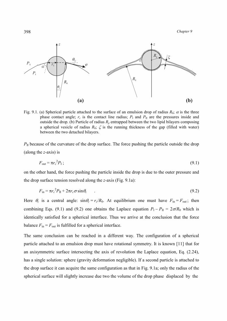
Fig. 9.1. (a) Spherical particle attached to the surface of an emulsion drop of radius R0; � is the threephase contact angle; rc is the contact line radius; PI and PII are the pressures inside andoutside the drop. (b) Particle of radius Rp entrapped between the two lipid bilayers composinga spherical vesicle of radius R0; � is the running thickness of the gap (filled with water)between the two detached bilayers.

PII because of the curvature of the drop surface. The force pushing the particle outside the drop

(along the z-axis) is

Fout = �rc2PI ; (9.1)

on the other hand, the force pushing the particle inside the drop is due to the outer pressure and

the drop surface tension resolved along the z-axis (Fig. 9.1a):

Fin = �rc2PII + 2�rc� sin�c . (9.2)

Here �c is a central angle: sin�c = rc/R0. At equilibrium one must have Fin = Fout ; then

combining Eqs. (9.1) and (9.2) one obtains the Laplace equation PI � PII = 2�/R0 which is

identically satisfied for a spherical interface. Thus we arrive at the conclusion that the force

balance Fin = Fout is fulfilled for a spherical interface.

The same conclusion can be reached in a different way. The configuration of a spherical

particle attached to an emulsion drop must have rotational symmetry. It is known [11] that for

an axisymmetric surface intersecting the axis of revolution the Laplace equation, Eq. (2.24),

has a single solution: sphere (gravity deformation negligible). If a second particle is attached to

the drop surface it can acquire the same configuration as that in Fig. 9.1a; only the radius of the

spherical surface will slightly increase due two the volume of the drop phase displaced by the


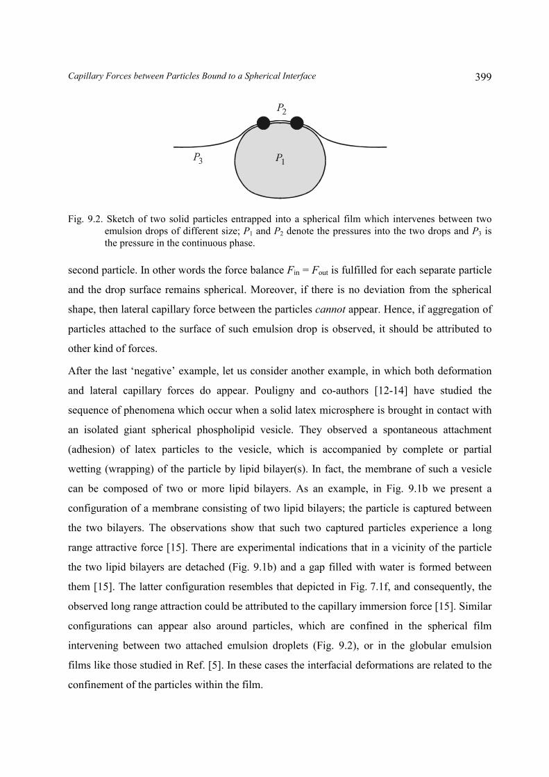
Fig. 9.2. Sketch of two solid particles entrapped into a spherical film which intervenes between twoemulsion drops of different size; P1 and P2 denote the pressures into the two drops and P3 isthe pressure in the continuous phase.

second particle. In other words the force balance Fin = Fout is fulfilled for each separate particle

and the drop surface remains spherical. Moreover, if there is no deviation from the spherical

shape, then lateral capillary force between the particles cannot appear. Hence, if aggregation of

particles attached to the surface of such emulsion drop is observed, it should be attributed to

other kind of forces.

After the last ‘negative’ example, let us consider another example, in which both deformation

and lateral capillary forces do appear. Pouligny and co-authors [12-14] have studied the

sequence of phenomena which occur when a solid latex microsphere is brought in contact with

an isolated giant spherical phospholipid vesicle. They observed a spontaneous attachment

(adhesion) of latex particles to the vesicle, which is accompanied by complete or partial

wetting (wrapping) of the particle by lipid bilayer(s). In fact, the membrane of such a vesicle

can be composed of two or more lipid bilayers. As an example, in Fig. 9.1b we present a

configuration of a membrane consisting of two lipid bilayers; the particle is captured between

the two bilayers. The observations show that such two captured particles experience a long

range attractive force [15]. There are experimental indications that in a vicinity of the particle

the two lipid bilayers are detached (Fig. 9.1b) and a gap filled with water is formed between

them [15]. The latter configuration resembles that depicted in Fig. 7.1f, and consequently, the

observed long range attraction could be attributed to the capillary immersion force [15]. Similar

configurations can appear also around particles, which are confined in the spherical film

intervening between two attached emulsion droplets (Fig. 9.2), or in the globular emulsion

films like those studied in Ref. [5]. In these cases the interfacial deformations are related to the

confinement of the particles within the film.

Chapter 9400

Fig. 9.3. Deformations in the membrane of a living cell due to (a) a microfilament pulling an inclusioninward and (b) a microtubule pushing an inclusion outward.

Looking for an example in biology, we could note that the cytoskeleton of a living cell is a

framework composed of interconnected microtubules and filaments, which resembles a

“tensegrity” architectural system composed of long struts joined with cables, see Refs. [16,17].

Moreover, inside the cell a gossamer network of contractile microfilaments pulls the cell’s

membrane toward the nucleus in the core [17]. In the points where the microfilaments are

attached to the membrane, concave “dimples” will be formed, see Fig. 9.3a. On the other hand,

at the points where microtubules (the “struts”) touch the membrane, the latter will acquire a

“pimple”-like shape, see Fig. 9.3b. Being deformations in the cell membrane, these “dimples”

and “pimples” will experience lateral capillary forces, both attractive and repulsive, which can

be employed to create a more adequate mechanical model of a living cell and, hopefully, to

explain the regular “geodesic forms” which appear in some biological structures [17].

Other example can be a lipid bilayer (vesicle) containing incorporated membrane proteins,

around which some local variation in the bilayer thickness can be created. The latter is due to

the mismatch in the thickness of the hydrophobic zones of the protein and the bilayer. The

overlap of such deformations can give rise to a membrane-mediated protein-protein interaction

[18]. A peculiarity of this system, which is considered in Chapter 10 below, is that the

hydrocarbon core of the lipid bilayer exhibits some elastic properties and cannot be treated as a

simple fluid [19,20].


Coming back to simpler systems, in which lateral capillary forces can be operative, we should

mention a configuration of two particles (Fig. 9.4b), which are confined in a liquid film wetting

a bigger spherical solid particle. The problem about the capillary forces experienced by such

two particles has been solved in Ref. [21]. The developed theoretical approach, which is

applicable (with possible modifications) also to the other systems mentioned above, is

described in the rest of the present chapter.

9.2. INTERFACIAL SHAPE AROUND INCLUSIONS IN A SPHERICAL FILM

9.2.1. LINEARIZATION OF LAPLACE EQUATION FOR SMALL DEVIATIONS FROM SPHERICAL SHAPE

Figure 9.4 shows schematically a spherical solid substrate (I) of radius Rs covered with a liquid

film (F) intervening between the substrate and the outer fluid phase (II). The film contains two

identical entrapped particles which deform the outer film surface. The non-disturbed spherical

liquid film can have a stable equilibrium thickness h0 only due to the action of some repulsive

forces (positive disjoining pressure) between the two film surfaces. For that reason a thin film,

Fig. 9.4. (a) Two ‘cork-shaped’ particles and (b) two spherical particles of radius Rp protruding from aliquid layer on a solid substrate of radius Rs ; the angles �a and �c characterize the particlepositions and size; rc is the contact line radius; hc is the elevation of the contact line above thelevel of the reference sphere of radius R0; � is the three-phase contact angle; in both (a) and(b) the meniscus slope angle �c is subtended between the normal to the segment ON and thetangent to the meniscus [21].

Chapter 9402

i.e. a film for which the effect of the disjoining pressure � is not negligible, is considered here.

Below we restrict our considerations to film thickness and particle size much smaller than Rs.

An auxiliary system is depicted in Fig. 9.4a, in which each of the two particles have the special

shape of a part of slender cone with vertex in the center of the substrate. In Ref. [21] it has been

demonstrated, that the consideration of such cork-shaped particles is useful for the subsequent

treatment of the more realistic system with two spherical particles depicted in Fig. 9.4b. We

will first present the results for cork-shaped particles, which will be further extended to

spherical particles in Section 9.3.3 below.

The deviation of the outer film surface (Fig. 9.4) from the spherical shape is caused by the

capillary rise of the liquid along the particle surface to form an equilibrium three-phase contact

angle �. For given radius of the substrate, film volume and particle shape there is one special

value �0 of the contact angle (Fig. 9.4b), which corresponds to spherical shape of the outer film

surface (�0 = �/2 for the configuration in Fig. 9.4a). The radius of this sphere is denoted by R0;

below it will be termed the reference sphere [21] and the interfacial deformations created by

the trapped particles (for � � �0) will be accounted with respect to this spherical surface.

The radial coordinate of a point of the deformed film surface can be presented in the form

r = R0 + �(�,�) (9.3)

where � and � are standard polar and azimuthal angles on the reference sphere r = R0 and

�(�,�) expresses the interfacial deformation due to the presence of the two particles. We

assume small deformations,

|� /R0| << 1 and |�II� |2 << 1, (9.4)

where �II denotes surface gradient operator in the reference sphere. At static conditions the

interfacial shape obeys the Laplace equation of capillarity, which in view of Eq. (9.4) can be

linearized [22,23]:

PR + �(h) � PII = �(h) ��

��

��

� 2II2

00

22RR

(9.5)


Here PII is the pressure in the outer fluid (II), PR is the reference pressure in the thin liquid film,

� is disjoining pressure and � is the interfacial tension of the boundary film�phase II. If the

liquid film contacts with a bulk liquid phase, as it is in Fig. 9.2, then the reference pressure can

be identified with the pressure in this phase, that is PR = P3 for the system depicted in Fig. 9.2.

On the other hand, if the film is closed as it is in Fig. 9.4, then PR can be determined from the

condition for constancy of the volume of this film, see Eq. (9.18) below. For ��0 Eq. (9.5)

reduces to the Laplace equation for the surface of a spherical thin liquid film, see Eqs. (6.8)-

(6.10) and Ref. [24].

Both � and � depend on the film thickness

h = h0 + � , h0 � R0 � Rs = const. (9.6)

Moreover, for a wetting film � and � are connected by means of the relationship [25]

�(h) = �� + �(h) dhh

�

� , (9.7)

where �� is the surface tension of the bulk liquid phase (infinitely thick film), see Eq. (5.8)

above. The integral term in Eq. (9.7) expresses the equilibrium work (per unit area) carried out

by the surface forces to bring the two film surfaces from infinity to a finite separation h. For

� << h0, using Eqs. (9.6) and (9.7), one can expand �(h) and �(h) in series:

� = �0 + �� + ..., � = �0 � �0� � 21��

2 + ..., (9.8)

where

�0 = � 0hh� , �0 = �

0hh� , �� = (d�/dh)0hh� , (9.9)

Next, we substitute Eq. (9.9) into Eq. (9.5) and obtain the linearized Laplace equation in the

form [21]

Hq �� 222II �� , (9.10)

where the following notation has been introduced:

Chapter 9404

00

0

00

2 22RR

q��

��

�� (9.11)

�H � 00 2

11,11�

��

RRR(PR + �0 � PII) (9.12)

Here q�1 has the meaning of capillary length, which determines the range of the interfacial

deformation and of the lateral capillary force; note that for R0� Eq. (9.11) reduces to the

form of Eq. (7.7) for flat thin films. On the other hand, if disjoining pressure is missing (as it is

for the systems depicted in Fig. 9.3) then q2 = �2/R0; in such a case q will be an imaginary

number and the Laplace equation, Eq. (9.10), will have oscillatory solutions. Following

Ref. [21], we will assume that the effect of disjoining pressure is predominant (this guarantees

the stability of the films in Figs. 9.2 or 9.4), and we work with real values of the parameter q.

Indeed, for stable films �� < 0 , see e.g. Ref. [26]; we assume that |�� | is large enough to have

q2 > 0.

In Eq. (9.12) �H stands for the change in the mean curvature of the film surface due to the

deformation caused by the two entrapped particles (Fig. 9.4); R can be interpreted as the outer

radius of an imaginary spherical layer of thickness h0, whose internal pressure is equal to the

pressure inside the perturbed film [21].

9.2.2. “CAPILLARY CHARGE” AND REFERENCE PRESSURE

�H and PR can be determined from the physical condition that the volume of the liquid film

does not change, i.e. the liquid within the film is incompressible and the phase boundaries are

closed for the exchange of molecules with the neighboring phases [21]. In such a case the

integral

��

��

��

�

00

0

0

20

3

0

22

3sin

SS

R

Rm RR

dsrdrddV ��

�

, (9.13)

expressing the change in the film volume due to the surface deformation, must be equal to zero;

the integration is taken over the surface domain S0 representing the radial projection of the

deformed film surface on the reference sphere; ds is a surface element. For the system with

cork-shaped particles (Fig. 9.4a) Vm = 0 is a rigorous relationship, whereas for the system with


spherical particles Vm = 0 is an approximate expression because the small volumes shown

shaded in Fig. 9.4b are neglected. Linearizing the integrand in Eq. (9.13) and substituting �

from Eq. (9.10) one derives [21]

0 = Vm ��

00

2II

2 (SS

dsqds �� 2�H) (9.14)

Further, from Eq. (9.14) one obtains

8�R02�H � ��

�

��

2

1IIIIII

~)(20 0 k CS S k

dldsHds �� n , (r0/R0)2 << 1 (9.15)

At the last step we have used the Green-Gauss-Ostrogradsky theorem, see e.g. Refs. [27-29]; Ck

(k = 1,2) are two circular contours representing the orthogonal (radial) projections of the two

particle contact lines onto the reference sphere of radius R0; dl is a linear element; ñ is a unit

running normal to Ck directed inwards. The linear integral yields

cC

rdlk

�� tan2~0II �� n , r0 � R0 sin�c (9.16)

where tan�c is the average meniscus slope at the contact line, see Fig. 9.4, and r0 is the radius

of the circumference Ck. In the case of fixed contact angle �, for the system depicted in

Fig. 9.4a �c = �/2 � � = const. and one can directly write ñ��II� = tan�c. Finally, combining

Eqs. (9.15) and (9.16) one obtains the sought-for expression for �H [21]:

�H Q/(2R02), Q � r0 sin�c r0 tan�c (sin2

�c << 1) (9.17)

Here, as usual, Q denotes the “capillary charge” of the entrapped particles, cf. Eqs. (7.9) and

(7.14). Finally, from Eqs. (9.12) and (9.17) one determines the reference pressure inside the

closed film [21]:

PR = PII � �0 + 2�0/R0 � �0Q/R02 (9.18)

Since �H is constant (independent of the surface coordinates � and �) it is convenient to

present Eq. (9.10) in the simpler form

��~~ 22

II q�� , (9.19)where

�~ � (� + 2q�2

�H)/R0 (9.20)

Chapter 9406

9.2.3. INTRODUCTION OF SPHERICAL BIPOLAR COORDINATES

To integrate conveniently Eq. (9.19) special bipolar coordinates on a sphere have been invented

in Ref. [21]. The connection between the Cartesian coordinates (x,y,z) and these curvilinear

coordinates (r,�,�) are:

Fig. 9.5. (a) Bipolar coordinate lines on the unit sphere: the lines � = const. are analogous to theparallels, while the lines � = const. connecting the two “poles” resemble meridians, cf. Eq.(9.21). (b) The parametrization of the reference sphere, r = R0 in Fig. 9.4, by means of sphericalbipolar coordinates reduces the integration domain of Eq. (9.19) to a rectangle; after Ref. [21].


� ��

��

��

��

��

��

coscoshcoscosh,

coscoshsin1,

coscoshsinh1 22

�

�

�

�

�

�

�

�

�

rzryrx (9.21)

The surfaces r = const. are spheres; the lines � = const. (on each sphere r = const.) are circum-

ferences which are counterparts of the meridians; the lines � = const. are circumferences �

counterparts of the parallels of latitude, see Fig. 9.5a. In each point on the sphere the respective

�-line and �-line are orthogonal to each other. These bipolar coordinates on a sphere induce

orthogonal biconical coordinates in space, which in fact are defined by Eq. (9.21). A detailed

description of these coordinates can be found in Ref. [21], including expressions for the

components of the metric tensor and Christoffel symbols, for various differential operators,

components of the rate-of-strain tensor and the respective form of the Navier-Stokes equation.

In the special case considered here we will use the spherical bipolar coordinates (�, �) for a

parametrization of the reference sphere r = R0 = const. In terms of these coordinates the surface

gradient operator acquires the form [21]

�II� = ��

��

��

��

��

��

��

��

ee1 (9.22)

where

��

coscosh �

�

a , a � R0 (2 � 1)1/2 (9.23)

e� and e� are the unit vectors of the local surface basis. With the help of the spherical bipolar

coordinates we bring Eq. (9.19) in the form [21]

(cosh� � cos�)2��

��

�� 2

2

2

2 ~~

��

��

��

�� = (qa)2�~ (�,�) (9.24)

where a is defined by Eq. (9.23); note that Eq. (9.24) much resembles Eq. (7.32). The

parameter , which depends on the distance between the two particles, is defined by means of

the expression [21]

a

c

�

��

coscos

� (�a � �c) (9.25)

Chapter 9408

Note that can vary in the interval 1 ; in particular, = 1 when the two particles in

Fig. 9.4a touch each other, while = when the particles are diametrically opposed. The

contact lines on the two particles correspond to � = ��c, where [21]:

�c � arctanh[(cos2�c � cos2

�a)1/2/sin�a] (�c �a �/2) (9.26)

Thus the integration domain of Eq. (9.24) acquires the simple form of a rectangle, see

Fig. 9.5b:

�� +�, ��c � +�c (9.27)

The boundary condition of fixed contact angle (stemming from the Young equation) for

the system depicted in Fig. 9.4a implies

ñ��II� = (�1)k tan�c at contour Ck (k = 1, 2) (9.28)

ñ has the same meaning as in Eq. (9.15); since Ck represents a line of fixed �-coordinate

(� = ��c), then ñ = �e� at the contour Ck. Thus with the help of Eqs. (9.20), (9.22) and (9.23) the

boundary condition (9.28) can be expressed in the form [21]

��

��

��

��

��

coscosh1sin~ 2

�

��

��

��

�

�c

c

c

(fixed contact angle) (9.29)

The boundary condition of fixed contact line has the same physical meaning as in

Sections 7.3.4 and 8.2.1: the position of the contact line is fixed at some edge on the particle

surface or at the boundary between hydrophilic and hydrophobic domains. In this case � = hc =

const. at the contact line, see Fig. 9.4. The linear elements along the �-lines and �-lines in

spherical bipolar coordinates are

dl� = d� , dl� = d� (9.30)

Taking into account Eqs. (9.16), (9.17), (9.20), (9.22) and (9.30), the boundary condition � = hc

can be expressed in terms of �~ [21]:

c��

�

~ = ��

��

��

��

�

��

��

��

� 020

20

~1

c

dRqR

hc (fixed contact line) (9.31)


Note that when the position of the contact line is fixed on the surface of an axisymmetric

particle, the exact shape of the particle (cork-like or spherical) is not important insofar as in all

cases the contact line is a circumference of a given fixed radius. In this aspect Eq. (9.31) is

applicable for both types of particles depicted in Fig. 9.4.

9.2.4. PROCEDURE OF CALCULATION AND NUMERICAL RESULTS

To obtain numerical results about the interfacial shape, and further to apply them to the

calculation of the lateral capillary force (Section 9.3 below), we first have to specify the input

parameters. It is convenient to scale all parameters using the reference radius R0 and the

interfacial tension �0 ; then in the computations one can work only in terms of dimensionless

parameters and variables. Thus the input parameters characterizing the film are h0/R0 and qR0.

The input parameters related to the confined particles are �a, �c and hc/R0 (or �) when the

contact line (or the contact angle) on the particle is fixed. Next, and �c are calculated by

means of Eqs. (9.25) and (9.26). In the considered case of spherical geometry the distance

between the two particles can be characterized by the length of the shortest arc connecting the

axes of the two particles: L = 2�aR0. In the numerical calculations it is convenient to use the

dimensionless distance

L~ � L/(�R0) = 2�a/� (2�c/� L~ 1) (9.32)

Note that the maximum value L~ = 1 corresponds to a configuration of two diametrically

opposed particles.

As already mentioned, the usage of spherical bipolar coordinates transforms the domain of

integration of Eq. (9.24) into a rectangle in the (�,�)-plane, which is bounded by the lines

� = �� and � = ��c, see Fig. 9.5b. Due to the symmetry it is enough to find the meniscus profile

�~ (�,�) only in a quarter of this rectangle, say in the quadrant 0

�

�, 0

�

�c. The

symmetry implies the following additional boundary conditions at the inner boundaries of the

quadrant:

0~

,0~~

00

��

��

��

��

��

��

��

��

�

��

��

��

��

��

��

�� (9.33)

Chapter 9410

The rectangular shape of the integration domain considerably simplifies and accelerates the

numerical solution of Eq. (9.24) obeying the boundary conditions (9.29) and (9.33), or

alternatively, (9.31) and (9.33). In Ref. [21] the conventional finite difference scheme of

second order was used for discretization of the boundary problem. In this way for each node of

the integration network one linear algebraic equation was obtained. The resulting set of

equations was solved by means of the Gauss-Seidel iterative method [30,31] combined with

successive over-relaxation (SOR) and the Chebyshev acceleration technique [32].

When the boundary condition for fixed contact line, Eq. (9.31), is used, the numerical

procedure can be simplified if one seeks a solution in the form [21]

�~ (�,�) = A f(�,�), A = const. (9.34)

The constant A is determined as follows. The function f(�,�) apparently satisfies Eq. (9.24) and

the boundary conditions (9.33) with f instead of �~ . Then one imposes the requirement

c��

�

~ = A orc

f��

= 1 (fixed contact line) (9.35)

Combining Eqs. (9.31) and (9.35) one determines the constant A :

A = 1

020

20

11�

� ��

�

��

��

�

� �

�

��

��

�c

fdRqR

hc (9.36)

One has to first solve (numerically) the boundary problem for f(�,�), then to calculate A from

Eq. (9.36) and finally to determine ),(~�� from Eq. (9.34).

When the boundary condition for fixed contact angle, Eq. (9.29), is used, the average elevation

of the contact line, hc, is not constant, but varies with the distance L between the two particles.

From the calculated meniscus shape one can determine hc by means of the equation [21]

20

20

2

0

sinsincoscosh

),(~

sin1~

Rqddl

Rhh cc

c

c

C cc

cc

k

��

��

��

��

��

�

�

�

�

�� (9.37)

where �c(�) expresses the position of the contact line on the particle surface:


Fig. 9.6. Plot of the dimensionless average capillary elevation, hc /R0, vs. the dimensionless distance L~

between two “cork-shaped” particles (Fig. 9.4a) calculated in Ref. [21] for three differentvalues of the parameter qR0 at fixed values of the angles �c = 2� and �c = 3�.

�c(�) � �(�,�c) (9.38)

As an illustrative example in Fig. 9.6 we show the dependence of the dimensionless elevation

ch~ on the dimensionless interparticle distance L~ for three different values of qR0 for cork-

shaped particles (Fig. 9.4a). The values of the other parameters, �c = 2� and �c = 3�, are the

same for the three curves in Fig. 9.6. The increase of ch~ with the decrease of L~ is due to the

increasing overlap of the menisci created by the two particles. Since q�1 is the characteristic

size (length) of the meniscus zone, at fixed L~ the overlap is greater (and consequently hc is

larger) when q�1 is greater, i.e. qR0 is smaller, see Fig. 9.6.

The overlap of the menisci around the two particles has also another consequence: in general

the contact line is inclined, i.e. it does not lie in a plane perpendicular to the particle axis. This

effect is similar to that with the two vertical cylinders in Fig. 7.10. For small particles (rc <<

R0) this inclination turns out to be very small. Indeed, it can be characterized by the angle �c

defined as follows [21]

cc

cc

c

ccc hr �

��

sin)~1(2)0(~)(~

2)0()(

tan�

�

�

�

� rc = (R0 + hc)sin�c (9.39)

Chapter 9412

Fig. 9.7. Plot of the inclination angle of contact line, �c, vs. the dimensionless interparticle distance L~

calculated in Ref. [21] for three different values of the angle �c determining the size of a‘cork-shaped’ particle (Fig. 9.4a); the values of the parameters qR0 = 5 and �c = 5� are fixed.

The dependence of the contact line inclination �c on the dimensionless interparticle separation

L~ is illustrated in Fig. 9.7 for three different values of �c for cork-shaped particles (Fig. 9.4a).

The values of the other parameters, qR0 = 5 and �c = 5�, are the same for the three curves in

Fig. 9.7. For two diametrically opposed particles the inclination disappears because of the

symmetry of the system, that is �c = 0 for L~ = 1, see Fig. 9.7. As seen in the figure �c is small

even for short separations L~ . This fact will be utilized in Section 9.3.3 below in the procedure

for calculating the lateral capillary force experienced by spherical particles.

9.3. CALCULATION OF THE LATERAL CAPILLARY FORCE

In Fig. 9.4 the particles are pressed against the solid substrate by the meniscus surface tension;

the resultant of the force applied on each particle along the normal to the substrate is

counterbalanced by the bearing reaction. Our aim below is to calculate the tangential

component of the capillary force Ft, which represents the lateral capillary force acting between

the two particles. Let ea be the unit vector of the particle axis. We denote by et a vector, which

is perpendicular to ea and belongs to the plane xz, see Fig. 9.4a. Then in view of Eqs.

(7.21)�(7.23) the contributions of surface tension and pressure to the lateral capillary force are

��

Ctt dlF �

� me)( , � ��

St

pt PdsF )()( ne , (9.40)


Ft = )(�tF + )( p

tF (9.41)

The integration in Eq. (9.40) is carried out along the three-phase contact line C and throughout

the particle surface S. As usual, n is the running outer unit normal to the particle surface and m

is the unit vector in the direction of the surface tension, see Fig. 9.4a; m is simultaneously

perpendicular to the contact line and tangential to the liquid interface. Following Ref. [21]

below we calculate Ft for the cases of fixed contact line and contact angle separately.

9.3.1. BOUNDARY CONDITION OF FIXED CONTACT LINE

This boundary condition reads (see Fig. 9.4):

� = hc = const. (at the contact line) (9.42)

In such a case the contact line is a circumference, which is perpendicular to the vector ea, i.e. to

the particle axis. Then the symmetry of the system implies )( ptF = 0. On the other hand, )(�

tF

is not zero insofar as the meniscus slope

tan� = c��

��

��

��

��

��

�1 (9.43)

varies along the contact line (this is a manifestation of contact angle hysteresis); is given by

Eq. (9.23). The unit vectors of the biconical coordinates, e� , e� and er (see Fig. 9.5a), form a

local basis in each point of the contact line. Then the unit vector in the direction of surface

tension can be expressed in the form

m = � e� cos� � er sin� (9.44)

Next, we introduce polar coordinates (�, ), with running unit vectors e� and e� , in the plane of

the contact line. Then for the points of the contact line one can write

e� = � e� cos�c + ea sin�c , er = e� sin�c + ea cos�c . (9.45)

Taking into account that et�e� = cos and et�ea = 0 we combine Eqs. (9.44) and (9.45) to obtain

et � m = (cos�c cos� � sin�c sin�)cos (9.46)

Chapter 9414

The assumption for small meniscus slope, Eq. (9.4), used by us implies that angle � is small;

then in view of Eq. (9.43) we can write

sin� c��

��

��

��

��

��

�1 cos� 1 � 2

121

c��

��

��

��

��

�(9.47)

Recalling that Ft(p) = 0, from Eqs. (9.40), (9.46) and (9.47) one obtains

Ft = � �0 rc ��

��

�

��

��

��

�

��

��

��

��

��

��

��

0

2

2 sin2cos1cosc

ccd (9.48)

where rc is given by Eq. (9.39) and higher order terms are neglected. The running angles and

� provide two alternative parametrizations of the contact line, connected as follows [21]:

��

��

�

�

��

��

coscosh)1cosh(,

coscosh1coscoshcos

2/122

�

�

�

�

�

�

c

c

c

c

dd (9.49)

A substitution of Eq. (9.49) into (9.48), in view of Eqs. (9.20) and (9.23), finally yields [21]:

��

��

�

�

��

�

�

��

��

�

��

�

��

��

��

��

�

��

��

��

0

2

2/1200

~

coscoshsin2~

)1(1)1coscosh(

cc

cct dRF (9.50)

Having solved numerically the boundary problem in the case of fixed contact line, see Eqs.

(9.34)�(9.36), one can further substitute the result for the computed function ),(~�� into

Eq. (9.50) to calculate the lateral capillary force by means of numerical integration. Results are

shown in Section 9.3.4 below.

9.3.2. BOUNDARY CONDITION OF FIXED CONTACT ANGLE

The main difference with the previous Section 9.3.1 is that the contact line in general does not

lie in a plane perpendicular to the particle axis, see Fig. 9.8. As a result )( ptF is no longer zero

and the interfacial tension � can vary along the contact line in accordance with Eq. (9.8). Thus

from Eqs. (9.8) and (9.40) one obtains [21]

� ��

Cctt dlF ...))(( 00

)( �� me (9.51)


where �c is defined by Eq. (9.38). First we derive expressions for calculating Ft in the case of

cork-shaped particles; the case of spherical particles is considered in Section 9.3.3 below.

The unit vector in direction of the surface tension at the contact line is

m = n cos�c + b sin�c , b � t � n , (9.52)

where, as usual, n is the outer unit normal to the particle surface, t is the running unit tangent to

the contact line; b is a binormal and �c = �/2 � � = const., see Fig. 9.8. The unit vectors et , ey

and ea form a basis, which can be used to express n:

n = et cos�c cos + ey cos�c sin � ea sin�c (9.53)

Let us denote by R the running position vector of a point from the contact line; then

rcc

Rt

eRRt )]([,10 ��

��

�� (9.54)

where

tc2 � (R0 + �c)2 sin2

�c + (d�c/d )2, er = et sin�c cos + ey sin�c sin + ea cos�c (9.55)

By means of Eqs. (9.52)�(9.55) one can prove that

et � m = c

ccc

c

tdRd

dd �

��

��

�

� sinsin)sin|(|sincos 22��

��

�� + cos�c cos�c cos (9.56)

Further we substitute Eq. (9.56) into Eq. (9.51) to obtain [21]:

Fig. 9.8. The right-hand-side cork-shaped particle in Fig. 9.4asketched in an enlarged scale: t is a unit vectortangential to the three-phase contact line; n is anouter unit normal to the particle surface; b = t � n isa binormal; m is the unit vector in the direction ofthe surface tension, which is tangential to the liquidmeniscus and normal to the contact line; � is thethree-phase contact angle.

Chapter 9416

)(�tF = �2�0cos�c(cos�c sin�c + sin�c) �

�

��

��

0

sindd

d c

+ cos�c ��

�

�

��

�

��

��

��

��

��

000

2

0

0 2cos cc r

dd

rd (9.57)

where higher-order terms have been neglected. To calculate )( ptF we integrate the pressure

throughout the lateral surface of the cork-shaped particle (Fig. 9.8); thus using Eqs. (9.40) and

(9.53) we get

)( ptF = �cos�c � ��

�

�

�

��

�

��

�

��

�

�

��

2

0II

2

0

0

1

cossinr

R

R

rRc

c

c

drrPdrrPd (9.58)

where r1 and r2 are boundaries of integration satisfying the relationship r1 �c( ) r2 for any ;

the exact choice of r1 and r2 is not important, because they drop out from the final expression

for )( ptF . Indeed, integrating in Eq. (9.58), substituting PR from Eq. (9.18), and neglecting

higher order terms one obtains [21]:

)( ptF = 2(�0 � 2�0/R0)r0 cos�c �

�

��

0

coscd (9.59)

Next, we integrate by parts in Eq. (9.59), and combine the result with Eqs. (9.41) and (9.57):

Ft = �2�0cos�c (cos�c sin�c � sin�c) ��

��

��

��

��

��

��

�

��

0

2

0

0

0

coscossinddd

rddd c

cc (9.60)

Note that the terms with �0 in Eqs. (9.57) and (9.59) cancel each other. The numerical

procedure from Section 9.2.4 gives ),(~�� ; therefore it is more convenient to rearrange

Eq. (9.60) using � instead of as integration variable; by means of Eqs. (9.20) and (9.49) one

obtains [21]:

tF~ = �2 (cos�c sin�c � sin�c)��

��

�

��

�

coscosh1cotsin~ 2

0 �

��

c

ac

ddd

� ��

��

�

��

�

��

��

�

�

0

2

2)1coscosh(

~

1

cosc

cc

dd

d (9.61)


where c�~ � ),(~

c�� and tF~ denotes the dimensionless lateral capillary force:

tF~ � Ft /(�0R0) (9.62)

To calculate the capillary force Ft one has to first determine ),(~�� solving numerically

Eq. (9.24) and then to use Eq. (9.50) or (9.61) depending on whether the case of fixed contact

line or angle, respectively, is considered.

Note that in the case of fixed contact angle Eq. (9.61) contains the derivative �~

� /�� and

consequently the capillary force Ft stems from the inclination of the contact line. In contrast,

when the contact line is fixed at the particle surface, Eq. (9.50) contains only the derivative

�~

� /�� and then Ft originates from the variation of meniscus slope along the contact line.

9.3.3. CALCULATION PROCEDURE FOR CAPILLARY FORCE BETWEEN SPHERICAL PARTICLES

As already mentioned, if the boundary condition for fixed contact line, Eq. (9.42) is used, then

the capillary force Ft is calculated from Eq. (9.50) in the same way for spherical particles

(Fig. 9.4b) and cork-shaped particles (Fig. 9.4a). Indeed, in both cases the contact line is an

immobile circumference perpendicular to the particle-substrate axis. In other words, if the

contact line is fixed, then Ft is identical for spherical and cork-shaped particles having the same

radius of the contact line.

In contrast, if the boundary condition for fixed contact angle, Eq. (9.29), is imposed, then the

contact line moves along the particle surface when the interparticle separation L varies. In

addition, when the two particles approach each other (i) the capillary elevation of the contact

line hc defined by Eq. (9.37) increases (Fig. 9.6), and (ii) the inclination angle �c defined by

Eq. (9.39) also increases. As demonstrated in Fig. 9.7 for not too small values of the separation

L the inclination angle is rather small (tan�c << 1) and the contact line is almost perpendicular

to the particle-substrate axis. This fact allows one to utilize the following approximate two-step

procedure, which is analogous to that used in Section 7.3.2 for the case of a planar interface.

At the first step, as a zeroth approximation one assumes that the contact line lies in a plane

perpendicular to the axis determined by angle �a (Fig. 9.4b). In such a case the contact line is a

circumference of radius rc elevated at a distance hc from the reference sphere of radius R0.

Chapter 9418

At the second step one formally replaces the sphere by a cork shaped particle having the same

values of �c, �c and hc, as well as of rc , �a , �c , etc. Next, one solves numerically Eq. (9.24),

along with the boundary conditions (9.29) and (9.33) and substitutes the result for ),(~�� in

Eq. (9.61) to calculate the capillary force Ft. The value of Ft thus obtained, which is accurate

for the cork-shaped particle, gives a first approximation for the capillary force exerted on the

spherical particle.

Note that for different values of the distance L between two spherical particles the contact

radius rc and the capillary elevation hc (Fig. 9.6) are different, and consequently, using the

above procedure we replace the sphere with different cork-shaped particles (with different �c).

This reflects the shrinking of the contact line on the spherical surface with the increase of hc.

The mathematical background of the above procedure is the following [21]. The radius of the

contact line rc can be related to the radius of the reference sphere R0 and the particle radius Rp

(Fig. 9.4b):

rc = R0 (1 + ch sin�c)sin�c = Rp sin(� + �c + �c) , (9.63)

We have introduced the notation ch � hc/(R0 sin�c); for the numerical calculations it is

important that ch is insensitive to the value of �c. The length of the segment OM in Fig. 9.4b

can be expressed in a similar way:

|OM| = R0 (1 + ch sin�c)cos�c = R0 � h0 + Rp [1 + cos(� + �c + �c)] , (9.64)

The angle � � � + �c + �c is also shown in Fig. 9.4b. From Eqs. (9.63) and (9.64) one

eliminates angle � and obtains:

�c(�c) = arcsin ((Y � 1)/ ch ) , (9.65)

where

Y � (1 � h0/R0 + Rp/R0)cos�c + [(Rp/R0)2 � (1 � h0/R0 + Rp/R0)2 sin2�c]1/2 (9.66)

Now we can formulate a procedure of calculations, which is based on the above equations [21]:

The input parameters are Rp/R0, h0/R0, qR0, � and �a.

Further, �c and �c are calculated as follows.


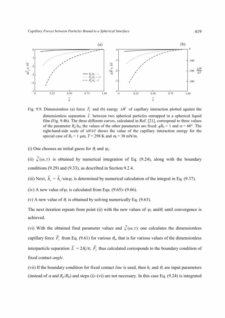
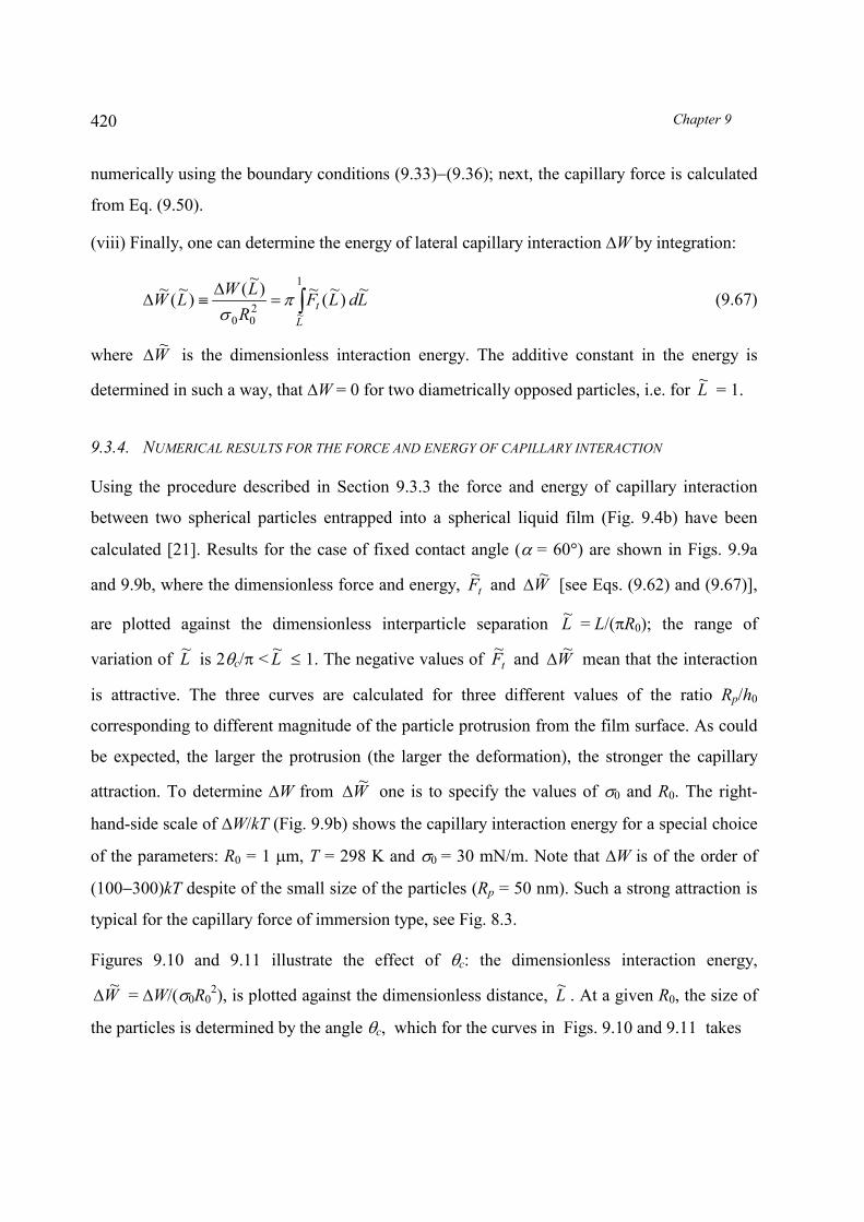
Fig. 9.9. Dimensionless (a) force tF~ and (b) energy W~� of capillary interaction plotted against thedimensionless separation L~ between two spherical particles entrapped in a spherical liquidfilm (Fig. 9.4b). The three different curves, calculated in Ref. [21], correspond to three valuesof the parameter Rp/h0; the values of the other parameters are fixed: qR0 = 1 and � = 60�. Theright-hand-side scale of �W/kT shows the value of the capillary interaction energy for thespecial case of R0 = 1 �m, T = 298 K and �0 = 30 mN/m.

(i) One chooses an initial guess for �c and �c.

(ii) ),(~�� is obtained by numerical integration of Eq. (9.24), along with the boundary

conditions (9.29) and (9.33), as described in Section 9.2.4.

(iii) Next, ch = ch~ /sin�c is determined by numerical calculation of the integral in Eq. (9.37).

(iv) A new value of�c is calculated from Eqs. (9.65)�(9.66).

(v) A new value of �c is obtained by solving numerically Eq. (9.63).

The next iteration repeats from point (ii) with the new values of �c and�c until convergence is

achieved.

(vi) With the obtained final parameter values and ),(~�� one calculates the dimensionless

capillary force tF~ from Eq. (9.61) for various �a, that is for various values of the dimensionless

interparticle separation L~ = 2�a/�; tF~ thus calculated corresponds to the boundary condition of

fixed contact angle.

(vii) If the boundary condition for fixed contact line is used, then hc and �c are input parameters

(instead of � and Rp/R0) and steps (i)�(vi) are not necessary. In this case Eq. (9.24) is integrated

Chapter 9420

numerically using the boundary conditions (9.33)�(9.36); next, the capillary force is calculated

from Eq. (9.50).

(viii) Finally, one can determine the energy of lateral capillary interaction �W by integration:

��

��

1

~200

~)~(~)~()~(~

Lt LdLF

RLWLW �

�

(9.67)

where W~� is the dimensionless interaction energy. The additive constant in the energy is

determined in such a way, that �W = 0 for two diametrically opposed particles, i.e. for L~ = 1.

9.3.4. NUMERICAL RESULTS FOR THE FORCE AND ENERGY OF CAPILLARY INTERACTION

Using the procedure described in Section 9.3.3 the force and energy of capillary interaction

between two spherical particles entrapped into a spherical liquid film (Fig. 9.4b) have been

calculated [21]. Results for the case of fixed contact angle (� = 60�) are shown in Figs. 9.9a

and 9.9b, where the dimensionless force and energy, tF~ and W~� [see Eqs. (9.62) and (9.67)],

are plotted against the dimensionless interparticle separation L~ = L/(�R0); the range of

variation of L~ is 2�c/� < L~ 1. The negative values of tF~ and W~� mean that the interaction

is attractive. The three curves are calculated for three different values of the ratio Rp/h0

corresponding to different magnitude of the particle protrusion from the film surface. As could

be expected, the larger the protrusion (the larger the deformation), the stronger the capillary

attraction. To determine �W from W~� one is to specify the values of �0 and R0. The right-

hand-side scale of �W/kT (Fig. 9.9b) shows the capillary interaction energy for a special choice

of the parameters: R0 = 1 �m, T = 298 K and �0 = 30 mN/m. Note that �W is of the order of

(100�300)kT despite of the small size of the particles (Rp = 50 nm). Such a strong attraction is

typical for the capillary force of immersion type, see Fig. 8.3.

Figures 9.10 and 9.11 illustrate the effect of �c: the dimensionless interaction energy,

W~� = �W/(�0R02), is plotted against the dimensionless distance, L~ . At a given R0, the size of

the particles is determined by the angle �c, which for the curves in Figs. 9.10 and 9.11 takes


Fig. 9.10. Case of fixed contact angle: dimensionless energy W~� of capillary interaction plotted

against the dimensionless separation L~ between two cork-shaped particles entrapped in a sphericalliquid film (Fig. 9.4a). The three curves, calculated in Ref. [21], correspond to three values of �c

denoted in the figure; the other parameters are �c = 5� and qR0 = 5. The right-hand-side scale of �W/kTis as in Fig. 9.9.

Fig. 9.11. Case of fixed contact line: dimensionless energy W~� of capillary interaction vs.

dimensionless separation L~ between two cork-shaped particles entrapped in a spherical liquidfilm (Fig. 9.4a). The three curves are calculated in Ref. [21] with the same values of �c as inFig. 9.10; for each curve hc/R0 is fixed and equal to the respective values of h� /R0 (0.00389,0.00585 and 0.00719) for the curves in Fig. 9.10. The right-hand-side scale of �W/kT is as inFig. 9.9.

Chapter 9422

values 1�, 2� and 3�, i.e. the particles are small, rc << R0. One sees again that the dimensional

interaction energy �W can be of the order of (10�100)kT. From a physical viewpoint

�W/kT >> 1 means that the capillary attraction prevails over the thermal motion and can bring

about particle aggregation and ordering in the spherical film.

Note that the parameters values in Figs. 9.10 and 9.11 are chosen in such a way, that the

shape of the fluid interfaces to be identical in the state of zero energy, i.e. for two diametrically

opposed particles. This provides a basis for quantitative comparison of the plots of �W vs. L~

in these two figures, calculated by using the two alternative boundary conditions. The curves in

Fig. 9.10 (as well as in Fig. 9.9) are calculated assuming fixed contact angle; one sees that the

interaction energy �W is always negative, i.e. corresponds to attraction. On the other hand, the

curves in Fig. 9.11 are calculated assuming fixed contact line. In the latter case the interaction

energy changes its sign at comparatively large interparticle distances: attractive at short

distances becomes repulsive at large separations.

The fact that that the interaction energy can change sign in the case of fixed contact line, but

the energy is always negative in the case of fixed contact angle, is discussed in Ref. [21]. It is

concluded that the non-monotonic behavior of the capillary interaction energy (Fig. 9.11) is a

non-trivial effect stemming from the spherical geometry of the film coupled with the boundary

condition of fixed contact line; such an effect is difficult to anticipate by physical insight. Note

that in the case of planar geometry the capillary force between identical particles is always

monotonic attraction.

9.4. SUMMARY

The fluid interfaces acquire spherical shape when the gravitational deformations are negligible.

Hence, lateral capillary forces of “flotation” type (Chapter 8), which are due to the particle

weight, do not appear between particles attached to a spherical interface, liquid film or

membrane. The capillary forces in this case can be only of “immersion” type (Chapter 7). In

such a case the origin of the interfacial deformation and the capillary force is the entrapment of

particles in the membrane of a spherical multilayered liposome (Fig. 9.1b), as well as in

“opened” (Fig. 9.2) and “closed” (Fig. 9.4) liquid films. Interfacial (membrane) deformations


and lateral capillary interactions can originate also from stresses due to outer bodies, like the

microfilament in Fig. 9.3a and the microtubule in Fig. 9.3b.

The calculation of the capillary force between particles trapped in spherical films is affected by

the specificity of the spherical geometry. For example, the condition for constancy of the

volume of the liquid in a closed spherical film (Fig. 9.4) leads to a connection between the

particle “capillary charge” Q and the pressure PR within the film, see Eq. (9.18). The stability

of such a film is provided by the repulsive disjoining pressure � exerted on its surfaces. The

disjoining pressure effect determines the capillary length q�1, see Eq. (9.11), and consequently,

the range of the lateral capillary forces. If disjoining pressure is missing (as it is in Fig. 9.3)

then q is an imaginary number and the Laplace equation, Eq. (9.19), has oscillatory solutions.

In our numerical solutions we have assumed that the effect of disjoining pressure is

predominant (this guarantees the stability of the films in Figs. 9.2 or 9.4), and we work with

real values of the parameter q.

The spherical bipolar coordinates, Eq. (9.21), represent the natural set of coordinates for the

mathematical description of the considered system: two axisymmetric particles entrapped into a

spherical liquid film. Thus the integration domain is reduced to a rectangle (Fig. 9.5) and the

numerical solution of the Laplace equation is made easier. The two types of boundary

conditions, fixed contact angle, Eq. (9.29), or fixed contact line, Eq. (9.31), lead to two

different expressions for the lateral capillary force, Eqs. (9.61) and (9.50), respectively. The

calculation of the capillary interaction between two spherical particles is more complicated in

the case of fixed contact angle due to the mobility of the contact line; to solve the problem in

Section 9.3.3 we have employed auxiliary cork-shaped particles. The interaction energy is

always negative (attractive) in the case of fixed contact angle (Figs. 9.9 and 9.10). On the other

hand, it turns out that the energy can change sign in the case of fixed contact line (attractive at

short distances but repulsive at long distances, Fig. 9.11). This non-monotonic behavior of the

capillary interaction energy is a non-trivial effect stemming from the specificity of the spherical

geometry coupled with the boundary condition of fixed contact line; such an effect does not

exist in the case of planar geometry, for which the capillary force between identical particles is

always monotonic attraction.

Chapter 9424

The magnitude of the capillary interaction energy can be of the order of 10�100 kT, see

Figs. 9.9 � 9.11, for sub-micrometer (Brownian) particles. In such a case, the capillary

attraction prevails over the thermal motion and can bring about particle aggregation and

ordering in the spherical film. In this respect, the physical situation is the same for spherical

and planar films, if only the particles are subjected to the action of the lateral immersion force.

9.5. REFERENCES

1. J. Sjöblom (Ed.), Emulsions and Emulsion Stability, M. Dekker, New York, 1996.

2. S. Hyde, S. Anderson, K. Larsson, Z. Blum, T. Landh, S. Lidin, B.W. Ninham, TheLanguage of Shape, Elsevier, Amsterdam, 1997.

3. A.G. Volkov, D.W. Deamer, D.L. Tanelian, V.S. Markin, Liquid Interfaces in Chemistryand Biology, Wiley, New York, 1998.

4. S. Hartland, Coalescence in Dense-Packed Dispersions, in: I.B. Ivanov (Ed.) Thin LiquidFilms, M. Dekker, New York, 1988; p. 663.

5. H. Wangqi, K.D. Papadopoulos, Colloids Surf. A 125 (1997) 181.

6. S.U. Pickering, J. Chem. Soc. 91 (1907) 2001.

7. Th. F. Tadros, B. Vincent, in: P. Becher (Ed.) Encyclopedia of Emulsion Technology,Vol. 1, Marcel Dekker, New York, 1983, p. 129.

8. N.D. Denkov, I.B. Ivanov, P.A. Kralchevsky, J. Colloid Interface Sci. 150 (1992) 589.

9. N. Yan, J.H. Masliyah, Colloids Surf. A 96 (1995) 229 and 243.

10. B.R. Midmore, Colloids Surf. A 132 (1998) 257.

11. H.M. Princen, The Equilibrium Shape of Interfaces, Drops, and Bubbles, in: E. Matijevic,(Ed.) Surface and Colloid Science, Vol. 2, Wiley, New York, 1969, p. 1.

12. C. Dietrich, M. Angelova, B. Pouligny, J. Phys. II France 7 (1997) 1651.

13. K. Velikov, C. Dietrich, A. Hadjiisky, K.D. Danov, B. Pouligny, Europhys. Lett. 40, (1997)405.

14. K. Velikov, K.D. Danov, M. Angelova, C. Dietrich, B. Pouligny, Colloids Surf. A, 149(1998) 245.


15. K.D. Danov, B. Pouligny, M.I. Angelova, P.A. Kralchevsky, "Strong Capillary Attractionbetween Spherical Inclusions in a Multilayered Lipid Membrane", in: Studies in SurfaceScience and Catalysis, Vol. 132, Elsevier, Amsterdam, 2001; pp. 519-524. See alsoK. D. Danov, B. Pouligny, P. A. Kralchevsky, "Capillary forces between colloidal particlesconfined in a liquid film: the finite-meniscus problem", Langmuir 17 (2001) 6599-6609.

16. D.E. Ingber, Ann. Rev. Physiol. 59 (1997) 575.

17. D.E. Ingber, Scientific American, January 1998, p. 30.

18. J.N. Israelachvili, Biochim. Biophys. Acta 469 (1977) 221.

19. A.G. Petrov, I. Bivas, Prog. Surface Sci. 16 (1984) 389.

20. P.A. Kralchevsky, V.N. Paunov, N.D. Denkov, K. Nagayama, J. Chem. Soc. FaradayTrans. 91 (1995) 3415.

21. P.A. Kralchevsky, V.N. Paunov, K. Nagayama, J. Fluid. Mech. 299 (1995) 105.

22. L.D. Landau, E.M. Lifshitz, Fluid Mechanics, Pergamon Press, Oxford, 1984.

23. P.A. Kralchevsky, I.B. Ivanov, J. Colloid Interface Sci. 137 (1990) 234.

24. I.B. Ivanov, P.A. Kralchevsky, Mechanics and thermodynamics of curved thin films, in:I.B. Ivanov (Ed.) Thin Liquid Films, M. Dekker, New York, 1988; p. 49.

25. I.B. Ivanov, B.V. Toshev, Colloid Polymer Sci. 253 (1975) 593.

26. B.V. Derjaguin, N.V. Churaev, V.M. Muller, V.M., Surface Forces, Plenum Press:Consultants Bureau, New York, 1987.

27. C.E. Weatherburn, Differential Geometry of Three Dimensions, Cambridge UniversityPress, Cambridge, 1939.

28. L. Brand, Vector and Tensor Analysis, Wiley, 1947.

29. A.J. McConnell, Application of Tensor Analysis, Dover, New York, 1957.

30. G.A. Korn, T.M. Korn, Mathematical Handbook, McGraw-Hill, New York, 1968.

31. A. Constantinides, Applied Numerical Methods with Personal Computers, McGraw-Hill,New York, 1987.

32. R.W. Hockney, J.W. Eastwood, Computer Simulation Using Particles, McGraw-Hill, NewYork, 1981.

Chapter 9 in the book: P.A. Kralchevsky and K. Nagayama ...

Documents

Transcript of Chapter 9 in the book: P.A. Kralchevsky and K. Nagayama ...