Chapter 8

The atmospheric environment

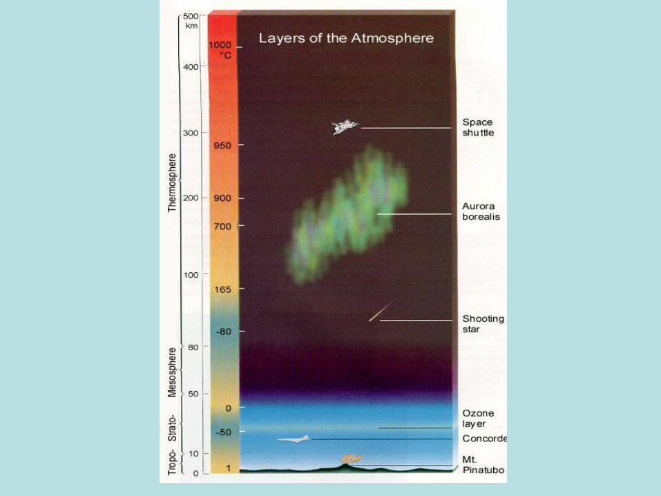
Figure 8-1. The U.S. Standard Atmosphere, 1976. Note the various temperature reversals, which act as thermal lids on the lower parts of the atmosphere. In the troposphere, gases are well mixed. From Neiburger et al. (1982).

TroposphereWell-mixed

ozone

Increasing temphere because of proximity to O3 layer

The atmosphere

Little mixingbetween the troposphere andstratosphere

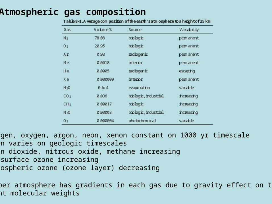
Atmospheric gas composition

Nitrogen, oxygen, argon, neon, xenon constant on 1000 yr timescaleOxygen varies on geologic timescalesCarbon dioxide, nitrous oxide, methane increasingNear surface ozone increasingStratospheric ozone (ozone layer) decreasing

Very upper atmosphere has gradients in each gas due to gravity effect on the different molecular weights

Solar Radiation and Atmospheric Heating

Solar constant – measure of the amount of energy passing through a unitsurface area perpendicular to the direction of the solar radiation

Albedo – amount of energy reflected back to space from the surface and the Atmosphere

Insolation – amount of energy reaching the earth’s surface

Incoming solar radiation is short-wavelengthOutgoing solar radiation is long-wavelength

Any gas with multiple bonds will absorb some long-wavelength radiation and turn it into heat…..greenhouse gas

Water vapor, carbon dioxide, nitrous oxide, methane, CFCs

Venus…

It is estimated that the surface temperature on Venus would actually be below 0°F without the Greenhouse effect. However, because of the greenhouse effect, the average surface temperature is 467°C or 872°F.

Atmospheric Composition at Surface Level

Major Components (by volume)

CO2 96.5%

N2 3.5%

Minor Component (ppm)

SO2 150

Ar 70

H2O 20

CO 17

He 12

Ne 7

Perfect Radiator: any substance that emits the maximum amount of electromagnetic energy at all wavelengths.

Total amount of energy emitted is a function of temperature and described by the Stefan-Boltzmann law:

E = T4

The wavelength of the maximum emitted energy varies inversely with the temperature and is described by the Wien displacement law:

M = aT-1

Short wavelength radiation: general term for radiation coming from the sun.

Long wavelength radiation: general term for radiation coming from the earth.

There is a latitudinal disequilibrium of heat on the planet

Figure 8-4. Incoming (shortwave) and outgoing (longwave) radiation as a function of latitude. The crossover occurs at ~40o. At lower latitudes there is a heat excess, at higher latitudes a heat deficit.

Yet the heat flux of the planet is just about in steady state. Heat redistributed due to atmospheric (and oceanic) circulation

Global Redistribution of Heat through circulation without the spin of the Earth

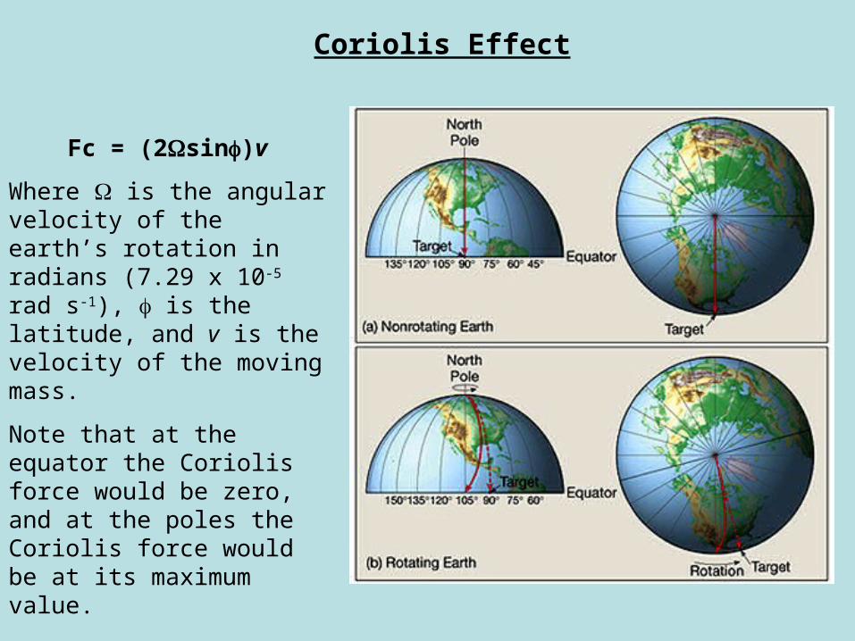
Coriolis Effect

Fc = (2sin)v

Where is the angular velocity of the earth’s rotation in radians (7.29 x 10-5 rad s-1), is the latitude, and v is the velocity of the moving mass.

Note that at the equator the Coriolis force would be zero, and at the poles the Coriolis force would be at its maximum value.

Global Atmospheric Circulation with the spin of the Earth

Ferrel Cell

Ferrel Cell

Polar Cell

Boston, MA latitude 42°23’ N

Death Valley, CA 36°34’N

Khartoum, Sudan 15°62’N

George town, Bahamas 23°51’ N

Macapá, Brazil 0°02’N

Wellington, New Zealand 41°26’S

Capitán Arturo Prat, Antarctica 62°33’

Reykjavik, Iceland 64°8’

Hydrostatic Equation: p = -gh

where p is the change in pressure, is the density of the fluid, g is the acceleration due to gravity, and h is the change in height.

Dry adiabatic lapse rate: the rate at which an air parcel cools if lifted in the atmosphere or warms if forced to lower levels, as long as no condensation occurs in the air parcel. (= ~9.8 K km-1.)

Absolute humidity: the amount of water vapor actually present in the air.

Relative humidity: the amount of water vapor in the air divided by the amount of water vapor the air can hold at any particular temperature, expressed in percent.

Wet adiabatic lapse rate: the rate at which an air parcel cools when condensation occurs. It is a function of temperature and pressure.

Environmental lapse rate: the observed rate at which temperature changes in a column of air.

Inversion: the reversal of the normal temperature pattern

Radiation inversion: caused by radiational cooling of the land surface and a decrease in the temperature of the atmosphere at low levels.

Subtropical inversion: caused by sinking air at high pressure center. *Remember, when air descends its temperature increases.

Frontal inversion: caused by the relative movement of warm air over cold air.

Air Pollution

Primary pollutants – direct products of combustion or evaporationVOCs, CO, CO2, SOx, NOx

Secondary pollutants – products of atmospheric reactions involving primary pollutants

Ozone, compounds produced by photochemical oxidation (PANs: Peroxyacytyl nitrate) VOCs and NOx’s are important reactants in forming secondary pollutants

Table 8-2. Classification of air pollutants

Major Class Subclass Examples

Inorganic gases Oxides of nitrogen N2O, NO, NO2

Oxides of sulfur SO2 , SO3

Oxides of carbon CO, CO2

Other inorganics O3 , H2S, HF, NH3, Cl2 , Rn

Organic gases Hydrocarbons Methane ( CH4), butane (C4H10), octane (C8H18),benzene (C6H6), acetylene (C2H2), ethylene (C2H4)

Aldehydes and ketones For maldehyde, acetone

Other organ ics Chlorofluorocarbons, PAHs, alcohols, organic acids

Particulates Solids Fume, dust, smoke, ash, carbon soot, lead, asbestos

Liquids Mist, spray, oil, grease, acids

AerosolsSolid particles or liquid droplets ranging in size up to 20um in radius. Caneither be put into the air directly or created in atm

SO2(g) + H2O H2SO4(l) Sulfuric acid aerosol

Table 8-3. Sources of aerosols an d contributions of natural versus anthropogenicsources*

SourceNatural

(1012 g y-1)Anthropogenic

(1012 g y-1)

Soil and rock dust 3000 - 4000 ?

Sea salt 1700 - 4700

Biogenic 100 - 500

Biomass burning (soot) 6 - 11 36 - 154

Volcanic 15 - 90

Direct emissions - fuel, incinerators, industry 15 - 90

Gaseous emissions

Su lfate from biogenic DMS 51

Su lfate from volcanic SO2 18 - 27

Su lfate from fossil fuel 105

Nitrate from NOx 62 128

Ammonium from NH3 28 37

Biogenic hydrocarbons 20 - 150

Anthropogenic hydrocarbons 100

Total 5000 - 9619 421 - 614

*Modified from Berner and Berner (1996)

Factoid: Following large volcanic eruptions, the sulfuric acid aerosol in the atmincreases the earth’s albedo leading to temporary global cooling

Table 8-3. Sources of aerosols an d contributions of natural versus anthropogenicsources*

SourceNatural

(1012 g y-1)Anthropogenic

(1012 g y-1)

Soil and rock dust 3000 - 4000 ?

Sea salt 1700 - 4700

Biogenic 100 - 500

Biomass burning (soot) 6 - 11 36 - 154

Volcanic 15 - 90

Direct emissions - fuel, incinerators, industry 15 - 90

Gaseous emissions

Su lfate from biogenic DMS 51

Su lfate from volcanic SO2 18 - 27

Su lfate from fossil fuel 105

Nitrate from NOx 62 128

Ammonium from NH3 28 37

Biogenic hydrocarbons 20 - 150

Anthropogenic hydrocarbons 100

Total 5000 - 9619 421 - 614

*Modified from Berner and Berner (1996)

Smog

Smoke + fogMore prevalent during inversions

Photochemical smogs – maximum during midday

Table 8-4. Types of s mogs an d their characteristics

Characteristic Industrial Photochemical

First occurrence London Los Angeles

Principal pollutants SOx O3, NOx, HC, CO, free radicals

Principal sources Industrial and household fuel combustion Motor vehicle fuel combustion

Effect on humans Lung and throat irritation Eye and respiratory irritation

Effect on compounds Reducing Oxidizing

Time of worst events Winter months in the early morning Summer months around midday

Industrial smog – mostly acid aerosols, corrode buildings and retinas

Photochemical smogs – mostly formation of ozone, NOx, and PAN, respiratory distress

The Great London Smog of 1952

Greenhouse Gases: CO2, CH4, N2O & CFCs that absorb long-wave, out-going radiation causing them to vibrate and generate heat.

Positive and negative feedbacks of greenhouse effect and climate change

Hotter world = more water vapor = more heat trapping = positive feedback

Hotter world = more cloud cover = less insolation = negative feedback

Hotter world = less snow = less albedo = more net insolation = postive feedback

Hotter world = faster decomp = more CO2 = more heat trap = positive feedback

More CO2 + temp = more photosynthesis = less CO2 = negative feedback

Geologic record indicates periods of warm wet earth and cold dry earth

The relative effect of an individual gas on the greenhouse effect over time depends upon:

Molecular scale radiative forcing (how well it converts radiation to heat)Atmospheric concentrationRate of increase in the atmosphereAtmospheric residence time

Table 8-5. Data for greenhouse gases*

GasConcen tration1990 (ppmv)

Positiveradiativeforcing(W m-2)

% total radiativeforcing

Lifetime(y)

Relativeinstantaneous

radiative forcing(molecular basis)

GlobalW armingPotential(100 y)

CO2 354 1.5 61 50 - 200 1 1

CH4 1.72 0.42 17 12 43 21

H2O strat - 0.14 6

N2O 0.310 0.1 4 120 250 310

CF C-11 0.00028 0.062 2.5 65 15,000 3,400

CF C-12 0.000484 0.14 6 130 19,000 7,100

Other CFCs 0.085 3.5

Total 2.45 100.0

CF C substitutes

HFC-23 264 650

HFC-152a 1.5 140

CF4 50,000 6,500

C6F14 3,200 7,400

*From Berner and Berner (1996), IPCC (1996), vanLoon and Duffy (2000)

CO2

Figure 8-8. Mean monthly concentrations of CO2 at Mauna Loa, Hawaii. From Berner and Berner (1996).

Imbalance = (fossil fuel) – (increase in CO2) – (ocean storage) + (deforestation)

The ‘missing’ carbon sink. The global CO2 budget is out of balance. We wouldpredict more increase in atm CO2 than what is actually observed.

Figure 8-9. The carbon cycle. Reservoir concentrations are in 1015 g (Gt) carbon. Fluxes are in Gt C y-1. From Berner and Berner (1996).

Fast

slow

Net reaction for atm CO2 uptake in ocean

CO2 + CO32- H2O + 2HCO3

-

Global C box modelRead Case Study 8-2

Methane2nd most important greenhouse gasSinks for methane:

1) chemical oxidation in the troposphere2) stratospheric oxidation3) microbe uptake

Figure 8-10. Variation in methane abundance from 1841 to 1996. The fitted curve is a sixth-order polynomial. Data from Etheridge et al. (1994) and IPCC (1966).

Table 8-7. Sources an d sinks for at mos pheric methane*

Source or Sink CH4 (1012 g C y-1) % total

Sources

Natu ral

Wetlands 86 22.5

Termites 15 3.9

Oceans 8 2.1

Lakes 4 1.0

Methane hydrates 4 1.0

Total natural 117 30.5

Anthropogenic

Energy production/use 69 18.0

Enteric fer mentation 63 16.4

Rice 45 11.8

Animal wastes 20 5.2

Landfills 29 7.6

Biomass burning 21 5.5

Domestic sewage 19 5.0

Total anthropogenic 266 69.5

Total fo r sources 383

Sinks

Atmospheric removal 353 88.2

Removal by soils 23 5.8

Atmosphere 24 6.0

Total fo r sinks 400

*Data from Berner and Berner (1996), IP CC (1992)

Methane

How could 14C help tell usThe source of atm methane?

Nitrous Oxide…its no laughing matter

N2O

Sources: denitrification, nitrification, biomass burning & fertilizer production

No N2O sinks in the troposphere

The third largest contributor to global warming behind CO2 and CH4.

Also responsible for stratospheric ozone destruction.

Climate Change and the Geologic Record

Ice coresStable isotopesDirect gas measurement of bubbles

Figure 8-11. Variation in temperature, CO2, and CH4 concentrations in Antarctica during the past 240,000 years. From Lorius et al. (1993).

Paleotemp fromisotopes

Climate Change and the Geologic Record

Sediment recordStable isotopes (oxygen and/ carbon)

Figure 8-12. Surface temperature of the Pacific Ocean based on oxygen isotope ratios. From THE BLUE PLANET, 2nd Edition by B. J. Skinner, S. C. Porter and D. B. Botkin. Copyright © 1999. This material is used by permission of John Wiley & Sons, Inc.

Oxygen isotopes in carbonatesfrom a sediment core in the WesternPacific

Several glacial / interglacial periods

OzoneGood ozone – stratosphereBad ozone – troposphere

Ozone production requires energy from photons

O2 + hv O* + O*

O* + O2 + M O3 (M is a catalyst …e.g. N; HR0 = -106.5 exothermic)

Net reaction …3O2 + hv 2O3

Ozone destruction also involves photonsO3 + hv O2 + O*O* + O3 O2 + O2

Figure 8-13. Absorption cross sections for oxygen and ozone in the 100 to 300 nm wavelengths. Also shown is the solar flux density and the wavelengths of biologically harmful radiation (UV-B and UV-C). From vanLoon and Duffy (2000).

Why good ozone is good.

Nitric acid in polar stratospheric clouds reacts with CFCs to form chlorine, which catalyzes the photochemical destruction of ozone. Chlorine concentrations build up during the winter polar night, and the consequent ozone destruction is greatest when the sunlight returns in spring (September/October). These clouds can only form at temperatures below about -80°C, so the warmer Arctic region does not have an ozone hole.

The polar vortex is a persistent, large-scale cyclone located near the Earth's poles, in the middle and upper troposphere and the stratosphere. It surrounds the polar highs and is part of the polar front.

Maximal ozone will form where form where gas molecule density and uv photondenisty are optimal.

Figure 8-14. Altitude versus variations in photon and molecular densities. The optimum altitude for ozone formation occurs where these curves cross.

Ozone layer

Stratospheric ozone distributionHigher over poles (stratospheric transport)Higher in summer vs. winter

The ozone hole

Figure 8-15. Seasonal variation of ozone concentrations (in Dobson units) at Halley Bay, Antarctica, for two different time periods. From Solomon (1990).

Hole varies in size dueto meteorological factors

Additions of N2O,CFCs, and bromineCompounds caused thedecline in ozone

Ozone destroying reactions

N2O

N2O + O* 2NONO + O3 NO2 + O2

NO2 + O NO + O2

O + O3 2O2

CFCl3

Cl’ + O3 ClO’ + O2

ClO’ + O Cl’ + O2

O + O3 2O2

CFCl3 + hv CFCl2’ + Cl’

For each of these reactionsthe Cl’ and the NO return to theiroriginal state. They are catalystsonly and do not participate in the reaction

Calculating reaction rates for various ozone destroying chemicals

Example 8-3: Calc reaction rate for Cl’ + O3 ClO’ + O3 at 235K.Cl’ conc. = 5.0 E11. O3 conc = 2.0 E12. Reaction rate = k [Cl][O3]

-Calc k using Arrhenius eqnk = Ae-Ea/RT

k = (2.8 E-12 cm3 molecules-1 s-1)e –(21 KJ mol-1)(8.314 kJ mol-1K-1)(235K)

k= 6.0 e-17 cm3 molecules-1 s-1

-Rate calcrate = (6.0 E-17 cm3 molecules-1 s-1)(5.0 E11 molecules cm-3)(2.0 E12 molecules cm-3)

rate = 6.0 E7 molecules cm-3 s-1

Tropospheric ozone

Bad ozonePhotochemical smogOH radicals or NO is a catalyst for the production of troposhperic ozone

NO (nitric oxide) released during fuel combustionNO converted to NO2 by a host of reactions

NO2 + hv NO + OO + O2 + M O3 + M …remember M is a catalytic particle

Figure 8-16. Variation in abundances of various species, on a 24-hour cycle, produced during a photochemical smog event. From vanLoon and Duffy (2000).

Of which, O3 is one

Radon – 222Rn

Produced from the 238U decay chainProblematic when bedrock contains uranium

218Po and 214Po progeny are particle active, particles inhaled, lodged in lungs…subsequent alpha decay damages lung tissue

Consider Rn levels inside:Generalized steady state equation for an inside pollutant

Ri = kexCi – kexCo

Ci = Co + Ri/kex

Ci = inside concCo = outside conckex = exchange coefRi= production rate of pollutant

Since Rn is radioactive, the expression is modified to acct. for decay

Ri= kex Ai + Ai – kexA0

Ai= (Ri + kexA0 ) / (kex + )

Indoor activity of Rn is:

Example 8-4: Radon release from soils to a basement at a rate of 0.01 Bq L-1 h-1

Outdoor air has Rn acitivity of 4.0 E-3 Bq L-1 h-1. Assume air exchange coeff of 10 h-1

What is the steady state indoor actvitiy of Rn?

Ai= (Ri + kexA0 ) / (kex + )

Plug and chug…answer is Ai = 5.0 E-3 Bq L-1 h-1

Radon flux depends on any factors that change gas diffusion-soil moisture-temp (solubility of Rn)-freezing (caps Rn)-barometric pressure

Rn is elevated in groundwaters and can be used as a tracer for gw inputs to Surface waters

Rainwater ChemistryCompounds found in rainwater come from seawater, terrestrial or pollution sources

Table 8-10. Sources of individual ions in rainwater*

Origin

Ion Marine inputs Terrestrial inputs Pollution inputs

Na+ Sea salt Soil dust Biomass burning

Mg2+ Sea salt Soil dust Biomass burning

K+ Sea salt Biogenic aerosolsSoil dust

Biomass burningFertilizer

Ca2+ Sea salt Soil dust Cement manufactureFuel burningBiomass burning

H+ Gas reaction Gas reaction Fuel burning

Cl- Sea salt None Industrial HCl

SO2

4 Sea saltDMS from biologicaldecay

DMS, H2S, etc., frombiological decayVolcanoesSoil dust

Biomass burning

NO

3 N2 plus lightning NO2 from biological decayN2 plus lightning

Auto emissionsFossil fuelsBiomass burningFertilizer

NH

4 NH3 from biologicalactivity

NH3 from bacterial decay NH3 fertilizersHuman, animal wastedecomposition(Combustion)

PO3

4 Biogenic aerosols adsorbedon sea salt

Soil dust Biomass burningFertilizer

HCO

3 CO2 in air CO2 in airSoil dust

None

SiO2, Al, Fe None Soil dust Land clearing

*From Berner and Berner (1996)

SO2

4

NO

3

NH

4

PO3

4

HCO

3

Cl- in rain is assumed tobe from a seawater source

Cl- and other ions in fromseawater are assumed to have a constant proportion

Rain sample can be ‘corrected’for seawater contribution

Excess ion X = total ion X – [(ratio of ion X to Cl- in seawater) (Cl- conc)]

Table 8-11. Weight ratios of major ions in seawater relative to Cl-- or Na++*

Ion W eight ratio to Cl- Weight ratio to Na+

Cl- 1.00 1.80

Na+ 0.56 1.00

Mg2+ 0.07 0.12

SO2

4 0.14 0.25

Ca2+ 0.02 0.04

K+ 0.02 0.04

*Source of data for ratio calculations, Wilson (1975)

Mg2+

SO2

4

Ca2+

Table 8-12. Primary associations for rainwater*

Origin Association

Marine Cl - Na - Mg - SO4

Soil Al - Fe - Si - Ca - (K, Mg, Na)

Biological N O3 - NH4 - SO4 - K

Biomass burning N O3 - NH4 - P - K - SO4 - (Ca, Na, Mg)

Industrial pollution SO4 - NO3 - Cl

Fertilizers K - PO4 - NH4 - NO3

*From Berner and Berner (1996)

Figure 8-17. Average Cl- concentration (mg L-1) of rainwater for the United States from July 1955 to June 1956. From Berner and Berner (1996).

Marine influence on rainwater chemistry

Marine influence on rainwater chemistry

Figure 8-18. Average Cl-/Na+ weight ratio of rainwater for the United States from July 1955 to June 1956. From Berner and Berner (1996).

SeawaterCl- /Na+ = 1.8

Low ratios reflectdust inputs from sodium-richrocks

Gaseous species

SO2(g) + 2OH(g) H2SO4(aq) 2 H+ + SO42- gas phase

SO2(g) + H2O2(aq) H2SO4(aq) 2H+ + SO42- liquid droplets

NO2(g) + OH(g) HNO3(aq) H+ + NO3-

NH3(g) + H2O NH4OH(aq) NH4+ + OH-

Acid depositionand what else?

Figure 8-19. Global SO2 produced by the burning of fossil fuel, 1940 to 1986, in Tg SO2 - S y-1 (1 Tg = 106 metric tons = 1012 g). From Berner and Berner (1996).

Figure 8-20. Global NOx produced by the burning of fossil fuel, 1970 to 1986, in Tg NOx - N y-1. From Berner and Berner (1996).

Figure 8-21. Generalized isoconcentration contours for SO42- (in mg L-1) for atmospheric precipitation over the

contiguous United States in 1995. Source of data is the NADP. From Langmuir (1997).

Figure 8-22. Generalized isoconcentration contours for NO3- (in mg L-1) for atmospheric precipitation over

the contiguous United States in 1995. Source of data is the NADP. From Langmuir (1997).

Figure 8-23. Average pH for precipitation in 1955-1956 and 1972-1973 for the northeastern United States and Canada and in 1980 for the contiguous United States and Canada. From Langmuir (1997).

Two most important species for acid rainare nitrate and sulfate

Example 8-7: Calc pH for a stream receiving acid rain.

Calc moles of sulfate and nitrate (from Table 8-13)sulfate = 2.165 E-5 mol L-1

nitrate = 2.355 E-5 mol L-1

Calculate H+ produced based on what you know about the normality of sulfuric andNitric acid. One mole H+ per mole nitrate, two moles H+ per mole sulfate.

Moles H+ = 6.685 E-5 mol L-1

pH = -log [H+] = 4.17

The Nitrogen Cycle

Hog Production in USA(1 dot= 10,000 Hogs and Pigs)

Chemistry and sources of atmospheric particulates (aerosols)

Figure 8-24. Sources of atmospheric particulates. Arrows with dashed lines indicate that there is a gaseous emission associated with the source.

Primarily tropospherictransport

Mineral dustFine particlesAeolian transportSahara dust

Trace element delivery to remote oceans (e.g. Antarctica)

Sea Salts

Bursting of bubblesPure sea salt aerosols have a predictable ratio of the major ions in seawater

Cl/Na , S/Na , N/Na

SulfatesSulfate aerosols can be in the form of (NH4)2SO4, or H2SO4 primarily

Sources: Anthropogenic - combustion Natural – DMS (dimethyl sulfide), volcanoes (SO2 and H2S)

Carbon-derived particleBlack carbon (soot) – incomplete combustion

Soot from coal (fly ash) = high K, Fe, Mn, ZnSoot from oil = high V

Organic aerosols- VOCsBioaerosols – spores, pollen, and volatile bio-organic compounds (Blue mountains)

Dry deposition – dust settlingRate determined by radius of particle (Stokes Law)

Wet deposition – washoutPrecip (rain or snow)Condensation

Aerosols serve as condensation nuclei for the formation ofclouds

Source tracking for aerosol deposition

Air mass trajectoriesUsing atmospheric circulation models to reconstruct the history of anair mass.

Aerosol : Crust Enrichment Factor

Determination of the amount of additional element that has been added to a particulate above that amount which you would expect based upon its crustalConcentration

Assume that the particulate conc. of Al, Fe, Si, Ti, or Sc are solely from the crustal contribution.

Calc EFcrust the crustal Enrichment Factor

XRE particulate

XRE crust

EFcrust=X = conc. of element XRE = conc. of reference element

Calculating the noncrustal conc. of element X

Xnoncrustal=XRE crust

- REparticulateXtotal

Table 8-14. Elemental composition of the continental crust*

Concentration (ppm) Concentration (ppm)

Element Upper crust Bulk crust Element Upper crust Bulk Crust

Al 80,400 84,100 Se 0.05 0.05

Fe 35,000 70,700 Mo 1.5 1.0

Sc 11 30 Ag 0.050 0.080

Ti 3000 5400 Cd 0.098 0.098

V 60 230 Sn 5.5 2.5

Cr 35 185 Sb 0.2 0.2

Mn 600 1400 W 2.0 1.0

Co 10 29 Au 0.0018 0.003

Ni 20 105 Pb 20 8.0

Cu 25 75 Th 10.7 3.5

Zn 71 80 U 2.8 0.91

As 1.5 1.0

*Data from Taylor and McLennan (1985). Both bulk continental crust and upper continentalcrust have been used to calculate crust ratios. In some cases the results may differsignificantly. For example, the Pb/Al ratio for the upper crust is 2.5 x 10 -4 while for the bulkcrust the ratio is 9.5 x 10 -5. Given a sample that has a Pb/Al ratio of 2.5 x 10 -4, the upper crustgives an EF of 1 while the bulk crust gives an EF of 2.6. The difference is great enough thatdifferent conclusions might be drawn regarding the source of the Pb (natural for upper crustnor malization and anthropogenic fo r bulk crust normalization). Cr would show an evengreater difference, but in the opposite sense. The Cr/Al ratio for the upper crust is 4.4 x 10 -4

while for the bulk crust the ratio is 2.2 x 10 -3. Given a sample with a Cr/Al ratio of 2.2 x 10 -3,the bulk crust normalization gives EF = 1 while the upper crust nor malization gives EF = 5suggesting that there is an anthropogenic contribution to the Cr content of the sample.

Example 8-9: Aerosol sample has 1000ppm Al and 7ppm Cr. Calculate the crustal enrichment factor and the noncrustal concentration of Cr

XRE particulate

XRE crust

EFcrust=

71,000 particulate

18584,100 crust

= = 3.2

Xnoncrustal=XRE crust

- REparticulateXtotal

Crnoncrustal= 18584,100- 10007

Crnoncrustal = 4.8 ppm

Elemental, molecular and isotopic signatures are used to source aerosols from crust, marine, or pollution sources

X = Xcrust + Xmarine + Xpollution

Using Al, Na, and Se, for reference elements for crust, marine, and pollution sourcesrespectively...

XAl crust

AlXSe pollution

SeXNa marine

NaX = + +

To solve for a particular component, divide both sides of equation by the ref elementfor that component. Ex: Crust

XAl crust

AlXSe pollution

SeXNa marine

NaX = + +

Al Al AlAl

Elemental

Pairwise plotting of the elemental ratios (X/Al, X/Na, X/Se) shows the contributionsof the different sources graphically

100% crustalsource

100% marinesource

100% crustalsource

100% pollutsource

Molecular signatures

‘Fingerprints’ mostly for VOCs

CPI (carbon preference index) = #odd carbon chains / #even carbon chainspetroleum= CPI = 1, natural compounds = CPI < 1

Chain length ratios, aromaticity, trace compounds, biomarkers

Isotopic signatures

Lead revisited- multiple lead isotopes that can be ratio-ed to each other and usedto derive other ratios.

Example 8-10: Aerosol sample: 206Pb/204Pb = 18.004, 208Pb/204Pb = 38.08, what’s the 208Pb / 206Pb ratio?

(208Pb/204Pb)(206Pb/204Pb) = 38.08/18.004 = 2.115

3 endmember mixing applied to lead isotopes

(207Pb/206Pb) meas = (207Pb/206Pb)a fa + (207Pb/206Pb)b fb + (207Pb/206Pb)c fc

Need two markers and 3 equations

1)

(206Pb/208Pb) meas = (206Pb/208Pb)a fa + (206Pb/208Pb)b fb + (206Pb/208Pb)c fc 2)

3) fa + fb + fc = 1

See Example 8-11

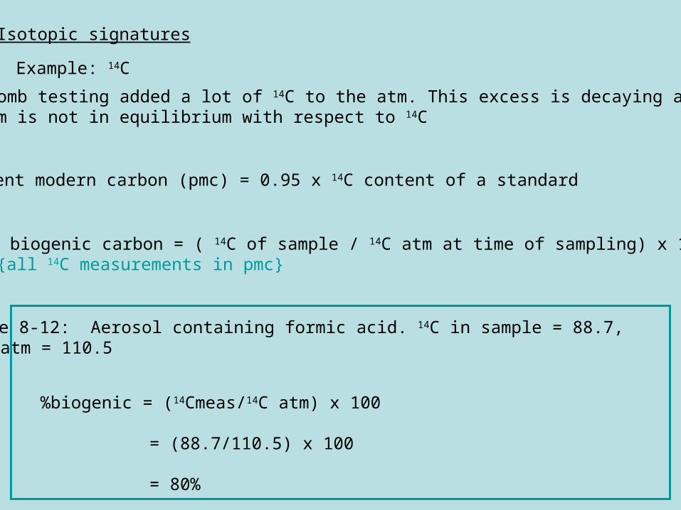
Isotopic signatures

Example: 14C

Percent modern carbon (pmc) = 0.95 x 14C content of a standard

Nuke bomb testing added a lot of 14C to the atm. This excess is decaying andthe atm is not in equilibrium with respect to 14C

Percent biogenic carbon = ( 14C of sample / 14C atm at time of sampling) x 100{all 14C measurements in pmc}

Example 8-12: Aerosol containing formic acid. 14C in sample = 88.7,14C in atm = 110.5

%biogenic = (14Cmeas/14C atm) x 100

= (88.7/110.5) x 100

= 80%

Happy Thanksgiving!!