Chapter 8 Speech Synthesis T - Columbia Universityjulia/courses/CS6998-2019/[08... ·...
38
DRAFT PRELIMINARY PROOFS. Unpublished Work c 2008 by Pearson Education, Inc. To be published by Pearson Prentice Hall, Pearson Education, Inc., Upper Saddle River, New Jersey. All rights reserved. Permission to use this unpublished Work is granted to individuals registering through [email protected] for the instructional purposes not exceeding one academic term or semester. Chapter 8 Speech Synthesis And computers are getting smarter all the time: Scientists tell us that soon they will be able to talk to us. (By ‘they’ I mean ‘computers’: I doubt scientists will ever be able to talk to us.) Dave Barry In Vienna in 1769, Wolfgang von Kempelen built for the Empress Maria Theresa the famous Mechanical Turk, a chess-playing automaton consisting of a wooden box filled with gears, and a robot mannequin sitting behind the box who played chess by moving pieces with his mechanical arm. The Turk toured Europe and the Americas for decades, defeating Napolean Bonaparte and even playing Charles Babbage. The Mechanical Turk might have been one of the early successes of artificial intelligence if it were not for the fact that it was, alas, a hoax, powered by a human chessplayer hidden inside the box. What is perhaps less well-known is that von Kempelen, an extraordinarily prolific inventor, also built between 1769 and 1790 what is definitely not a hoax: the first full-sentence speech synthesizer. His device consisted of a bellows to simulate the lungs, a rubber mouthpiece and a nose aperature, a reed to simulate the vocal folds, various whistles for each of the fricatives. and a small auxiliary bellows to provide the puff of air for plosives. By moving levers with both hands, opening and closing various openings, and adjusting the flexible leather ‘vocal tract’, different consonants and vowels could be produced. More than two centuries later, we no longer build our speech synthesizers out of wood, leather, and rubber, nor do we need trained human operators. The modern task of speech synthesis, also called text-to-speech or TTS, is to produce speech (acoustic Speech synthesis Text-to-speech TTS waveforms) from text input. Modern speech synthesis has a wide variety of applications. Synthesizers are used, together with speech recognizers, in telephone-based conversational agents that con- duct dialogues with people (see Ch. 23). Synthesizer are also important in non- conversational applications that speak to people, such as in devices that read out loud for the blind, or in video games or children’s toys. Finally, speech synthesis can be used to speak for sufferers of neurological disorders, such as astrophysicist Steven Hawking who, having lost the use of his voice due to ALS, speaks by typing to a speech synthe- sizer and having the synthesizer speak out the words. State of the art systems in speech synthesis can achieve remarkably natural speech for a very wide variety of input situa- tions, although even the best systems still tend to sound wooden and are limited in the voices they use. The task of speech synthesis is to map a text like the following: (8.1) PG&E will file schedules on April 20. to a waveform like the following:
Transcript of Chapter 8 Speech Synthesis T - Columbia Universityjulia/courses/CS6998-2019/[08... ·...
DRAFT
P R E L I M I N A R Y P R O O F S .Unpublished Work c©2008 by Pearson Education, Inc. To be published by Pearson Pr entice Hall,Pearson Education, Inc., Upper Saddle River, New Jersey. Al l rights reserved. Permission to usethis unpublished Work is granted to individuals registerin g through [email protected] the instructional purposes not exceeding one academic t erm or semester.
Chapter 8Speech Synthesis
And computers are getting smarter all the time: Scientists tell us that soon they will beable to talk to us. (By ‘they’ I mean ‘computers’: I doubt scientists will ever be able totalk to us.)
Dave Barry
In Vienna in 1769, Wolfgang von Kempelen built for the Empress Maria Theresa thefamous Mechanical Turk, a chess-playing automaton consisting of a wooden box filledwith gears, and a robot mannequin sitting behind the box who played chess by movingpieces with his mechanical arm. The Turk toured Europe and the Americas for decades,defeating Napolean Bonaparte and even playing Charles Babbage. The MechanicalTurk might have been one of the early successes of artificial intelligence if it were notfor the fact that it was, alas, a hoax, powered by a human chessplayer hidden inside thebox.
What is perhaps less well-known is that von Kempelen, an extraordinarily prolificinventor, also built between 1769 and 1790 what is definitelynot a hoax: the firstfull-sentence speech synthesizer. His device consisted ofa bellows to simulate thelungs, a rubber mouthpiece and a nose aperature, a reed to simulate the vocal folds,various whistles for each of the fricatives. and a small auxiliary bellows to providethe puff of air for plosives. By moving levers with both hands, opening and closingvarious openings, and adjusting the flexible leather ‘vocaltract’, different consonantsand vowels could be produced.
More than two centuries later, we no longer build our speech synthesizers out ofwood, leather, and rubber, nor do we need trained human operators. The modern taskof speech synthesis, also calledtext-to-speechor TTS, is to produce speech (acousticSpeech synthesis
Text-to-speech
TTS
waveforms) from text input.Modern speech synthesis has a wide variety of applications.Synthesizers are used,
together with speech recognizers, in telephone-based conversational agents that con-duct dialogues with people (see Ch. 23). Synthesizer are also important in non-conversational applications that speakto people, such as in devices that read out loudfor the blind, or in video games or children’s toys. Finally,speech synthesis can be usedto speakfor sufferers of neurological disorders, such as astrophysicist Steven Hawkingwho, having lost the use of his voice due to ALS, speaks by typing to a speech synthe-sizer and having the synthesizer speak out the words. State of the art systems in speechsynthesis can achieve remarkably natural speech for a very wide variety of input situa-tions, although even the best systems still tend to sound wooden and are limited in thevoices they use.
The task of speech synthesis is to map a text like the following:
(8.1) PG&E will file schedules on April 20.
to a waveform like the following:
DRAFT
250 Chapter 8. Speech Synthesis
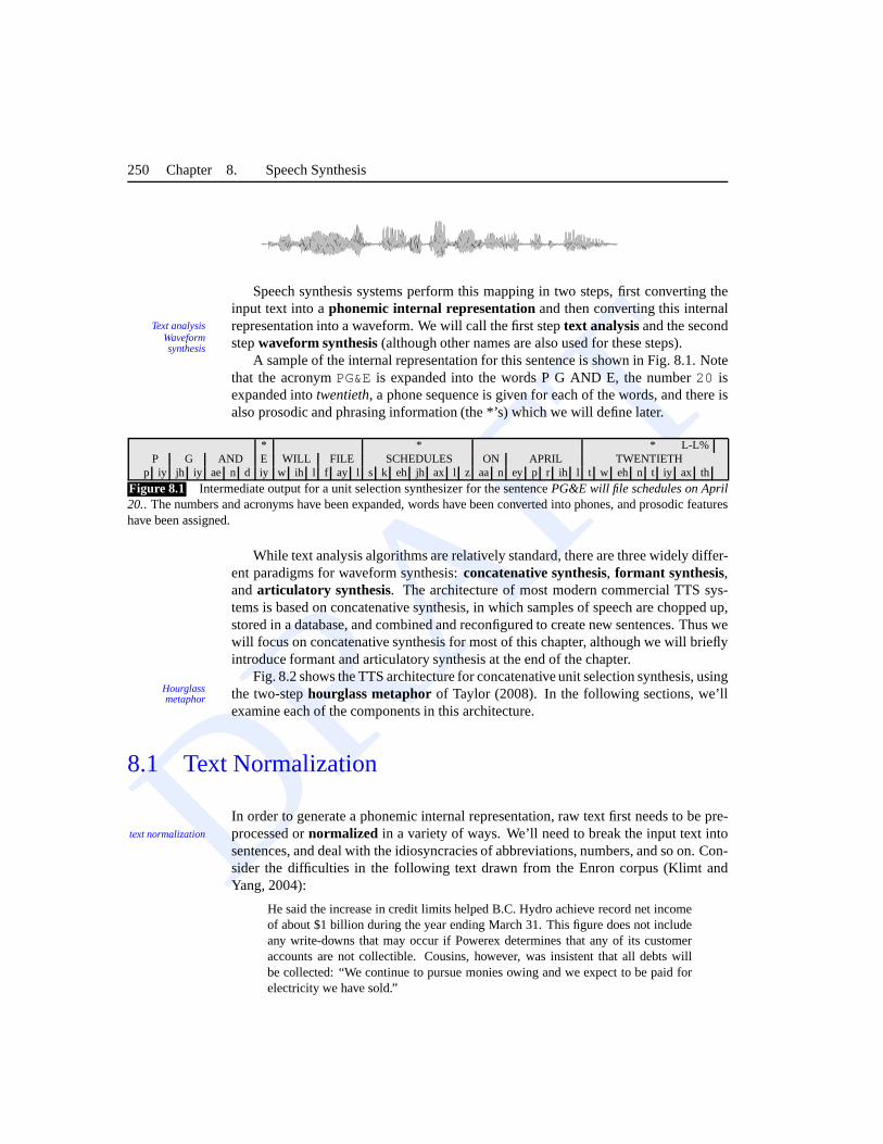
Speech synthesis systems perform this mapping in two steps,first converting theinput text into aphonemic internal representationand then converting this internalrepresentation into a waveform. We will call the first steptext analysisand the secondText analysis
stepwaveform synthesis(although other names are also used for these steps).Waveformsynthesis
A sample of the internal representation for this sentence isshown in Fig. 8.1. Notethat the acronymPG&Eis expanded into the words P G AND E, the number20 isexpanded intotwentieth, a phone sequence is given for each of the words, and there isalso prosodic and phrasing information (the *’s) which we will define later.
* * * L-L%P G AND E WILL FILE SCHEDULES ON APRIL TWENTIETH
p iy jh iy ae n d iy w ih l f ay l s k eh jh ax l z aa n ey p r ih l t w eh n t iy ax th
Figure 8.1 Intermediate output for a unit selection synthesizer for the sentencePG&E will file schedules on April20.. The numbers and acronyms have been expanded, words have been converted into phones, and prosodic featureshave been assigned.
While text analysis algorithms are relatively standard, there are three widely differ-ent paradigms for waveform synthesis:concatenative synthesis, formant synthesis,andarticulatory synthesis. The architecture of most modern commercial TTS sys-tems is based on concatenative synthesis, in which samples of speech are chopped up,stored in a database, and combined and reconfigured to createnew sentences. Thus wewill focus on concatenative synthesis for most of this chapter, although we will brieflyintroduce formant and articulatory synthesis at the end of the chapter.
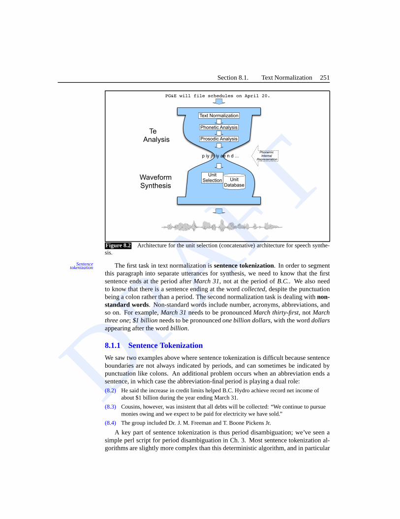
Fig. 8.2 shows the TTS architecture for concatenative unit selection synthesis, usingthe two-stephourglass metaphorof Taylor (2008). In the following sections, we’llHourglass
metaphorexamine each of the components in this architecture.
8.1 Text Normalization
In order to generate a phonemic internal representation, raw text first needs to be pre-processed ornormalized in a variety of ways. We’ll need to break the input text intotext normalization
sentences, and deal with the idiosyncracies of abbreviations, numbers, and so on. Con-sider the difficulties in the following text drawn from the Enron corpus (Klimt andYang, 2004):
He said the increase in credit limits helped B.C. Hydro achieve record net incomeof about $1 billion during the year ending March 31. This figure does not includeany write-downs that may occur if Powerex determines that any of its customeraccounts are not collectible. Cousins, however, was insistent that all debts willbe collected: “We continue to pursue monies owing and we expect to be paid forelectricity we have sold.”
DRAFTSection 8.1. Text Normalization 251
e
Analysis
Waveform Synthesis
PG&E will file schedules on April 20.
p iy jh iy ae n d ...
Text Normalization
Phonetic Analysis
Prosodic Analysis
UnitDatabase
Unit Selection
PhonemicInternal
Represenation
Figure 8.2 Architecture for the unit selection (concatenative) architecture for speech synthe-sis.
The first task in text normalization issentence tokenization. In order to segmentSentencetokenization
this paragraph into separate utterances for synthesis, we need to know that the firstsentence ends at the period afterMarch 31, not at the period ofB.C.. We also needto know that there is a sentence ending at the wordcollected, despite the punctuationbeing a colon rather than a period. The second normalizationtask is dealing withnon-standard words. Non-standard words include number, acronyms, abbreviations, andso on. For example,March 31needs to be pronouncedMarch thirty-first, not Marchthree one; $1 billion needs to be pronouncedone billion dollars, with the worddollarsappearing after the wordbillion.
8.1.1 Sentence Tokenization
We saw two examples above where sentence tokenization is difficult because sentenceboundaries are not always indicated by periods, and can sometimes be indicated bypunctuation like colons. An additional problem occurs whenan abbreviation ends asentence, in which case the abbreviation-final period is playing a dual role:(8.2) He said the increase in credit limits helped B.C. Hydro achieve record net income of
about $1 billion during the year ending March 31.
(8.3) Cousins, however, was insistent that all debts will be collected: “We continue to pursuemonies owing and we expect to be paid for electricity we have sold.”
(8.4) The group included Dr. J. M. Freeman and T. Boone Pickens Jr.
A key part of sentence tokenization is thus period disambiguation; we’ve seen asimple perl script for period disambiguation in Ch. 3. Most sentence tokenization al-gorithms are slightly more complex than this deterministicalgorithm, and in particular
DRAFT
252 Chapter 8. Speech Synthesis
are trained by machine learning methods rather than being hand-built. We do this byhand-labeling a training set with sentence boundaries, andthen using any supervisedmachine learning method (decision trees, logistic regression, SVM, etc) to train a clas-sifier to mark the sentence boundary decisions.
More specifically, we could start by tokenizing the input text into tokens separatedby whitespace, and then select any token containing one of the three characters! , . or? (or possibly also: ). After hand-labeling a corpus of such tokens, then we trainaclassifier to make a binary decision (EOS (end-of-sentence)versus not-EOS) on thesepotential sentence boundary characters inside these tokens.
The success of such a classifier depends on the features that are extracted for theclassification. Let’s consider some feature templates we might use to disambiguatethesecandidatesentence boundary characters, assuming we have a small amount oftraining data, labeled for sentence boundaries:
• the prefix (the portion of the candidate token preceding the candidate)• the suffix (the portion of the candidate token following the candidate)• whether the prefix or suffix is an abbreviation (from a list)• the word preceding the candidate• the word following the candidate• whether the word preceding the candidate is an abbreviation• whether the word following the candidate is an abbreviation
Consider the following example:
(8.5) ANLP Corp. chairman Dr. Smith resigned.
Given these feature templates, the feature values for the period . in the wordCorp.in (8.5) would be:
PreviousWord = ANLP NextWord = chairmanPrefix = Corp Suffix = NULLPreviousWordAbbreviation = 1 NextWordAbbreviation = 0
If our training set is large enough, we can also look for lexical cues about sen-tence boundaries. For example, certain words may tend to occur sentence-initially, orsentence-finally. We can thus add the following features:
• Probability[candidate occurs at end of sentence]• Probability[word following candidate occurs at beginningof sentence]
Finally, while most of the above features are relatively language-independent, wecan use language-specific features. For example, in English, sentences usually beginwith capital letters, suggesting features like the following:
• case of candidate: Upper, Lower, AllCap, Numbers• case of word following candidate: Upper, Lower, AllCap, Numbers
Similary, we can have specific subclasses of abbreviations,such as honorifics ortitles (e.g., Dr., Mr., Gen.), corporate designators (e.g., Corp., Inc.), or month-names(e.g., Jan., Feb.).
Any machine learning method can be applied to train EOS classifiers. Logisticregression and decision trees are two very common methods; logistic regression may
DRAFTSection 8.1. Text Normalization 253
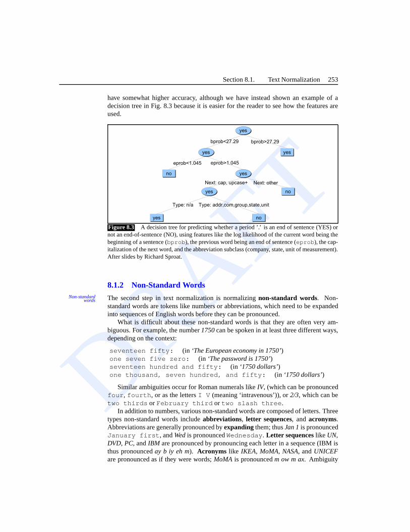
have somewhat higher accuracy, although we have instead shown an example of adecision tree in Fig. 8.3 because it is easier for the reader to see how the features areused.
Figure 8.3 A decision tree for predicting whether a period ’.’ is an end of sentence (YES) ornot an end-of-sentence (NO), using features like the log likelihood of the current word being thebeginning of a sentence (bprob ), the previous word being an end of sentence (eprob ), the cap-italization of the next word, and the abbreviation subclass(company, state, unit of measurement).After slides by Richard Sproat.
8.1.2 Non-Standard Words
The second step in text normalization is normalizingnon-standard words. Non-Non-standardwords
standard words are tokens like numbers or abbreviations, which need to be expandedinto sequences of English words before they can be pronounced.
What is difficult about these non-standard words is that theyare often very am-biguous. For example, the number1750can be spoken in at least three different ways,depending on the context:
seventeen fifty: (in ‘The European economy in 1750’)one seven five zero: (in ‘The password is 1750’)seventeen hundred and fifty: (in ‘1750 dollars’)one thousand, seven hundred, and fifty: (in ‘1750 dollars’)
Similar ambiguities occur for Roman numerals likeIV, (which can be pronouncedfour , fourth , or as the lettersI V (meaning ‘intravenous’)), or2/3, which can betwo thirds or February third or two slash three .
In addition to numbers, various non-standard words are composed of letters. Threetypes non-standard words includeabbreviations, letter sequences, andacronyms.Abbreviations are generally pronounced byexpandingthem; thusJan 1is pronouncedJanuary first , andWedis pronouncedWednesday . Letter sequenceslike UN,DVD, PC,andIBM are pronounced by pronouncing each letter in a sequence (IBMisthus pronounceday b iy eh m). Acronyms like IKEA, MoMA, NASA, andUNICEFare pronounced as if they were words;MoMA is pronouncedm ow m ax. Ambiguity
DRAFT
254 Chapter 8. Speech Synthesis
occurs here as well; shouldJanbe read as a word (the nameJan ) or expanded as themonthJanuary ?
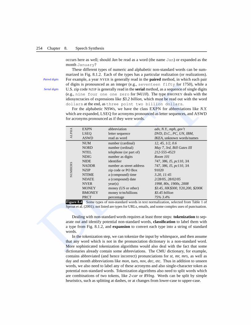
These different types of numeric and alphabetic non-standard words can be sum-marized in Fig. 8.1.2. Each of the types has a particular realization (or realizations).For example, a yearNYER is generally read in thepaired method, in which each pairPaired digits
of digits is pronounced as an integer (e.g.,seventeen fifty for 1750), while aU.S. zip codeNZIP is generally read in theserial method, as a sequence of single digitsSerial digits
(e.g.,nine four one one zero for 94110). The typeBMONEY deals with theidiosyncracies of expressions like$3.2 billion, which must be read out with the worddollars at the end, asthree point two billion dollars .
For the alphabetic NSWs, we have the class EXPN for abbreviations like N.Y.which are expanded, LSEQ for acronyms pronounced as letter sequences, and ASWDfor acronyms pronounced as if they were words.
AL
PH
A EXPN abbreviation adv, N.Y., mph, gov’tLSEQ letter sequence DVD, D.C., PC, UN, IBM,ASWD read as word IKEA, unknown words/names
NU
MB
ER
S
NUM number (cardinal) 12, 45, 1/2, 0.6NORD number (ordinal) May 7, 3rd, Bill Gates IIINTEL telephone (or part of) 212-555-4523NDIG number as digits Room 101NIDE identifier 747, 386, I5, pc110, 3ANADDR number as street address 747, 386, I5, pc110, 3ANZIP zip code or PO Box 91020NTIME a (compound) time 3.20, 11:45NDATE a (compound) date 2/28/05, 28/02/05NYER year(s) 1998, 80s, 1900s, 2008MONEY money (US or other) $3.45, HK$300, Y20,200,$200KBMONEY money tr/m/billions $3.45 billionPRCT percentage 75% 3.4%
Figure 8.4 Some types of non-standard words in text normalization, selected from Table 1 ofSproat et al. (2001); not listed are types for URLs, emails, and some complex uses of punctuation.
Dealing with non-standard words requires at least three steps: tokenization to sep-arate out and identify potential non-standard words,classificationto label them witha type from Fig. 8.1.2, andexpansionto convert each type into a string of standardwords.
In the tokenization step, we can tokenize the input by whitespace, and then assumethat any word which is not in the pronunciation dictionary isa non-standard word.More sophisticated tokenization algorithms would also deal with the fact that somedictionaries already contain some abbreviations. The CMU dictionary, for example,contains abbreviated (and hence incorrect) pronunciations for st, mr, mrs, as well asday and month abbreviations likemon, tues, nov, dec, etc. Thus in addition to unseenwords, we also need to label any of these acronyms and also single-character token aspotential non-standard words. Tokenization algorithms also need to split words whichare combinations of two tokens, like2-car or RVing. Words can be split by simpleheuristics, such as splitting at dashes, or at changes from lower-case to upper-case.
DRAFTSection 8.1. Text Normalization 255
The next step is assigning a NSW type; many types can be detected with simpleregular expressions. For example,NYER could be detected by the following regularexpression:
/(1[89][0-9][0-9])|(20[0-9][0-9]/
Other classes might be harder to write rules for, and so a morepowerful option isto use a machine learning classifier with many features.
To distinguish between the alphabeticASWD, LSEQandEXPN classes, for examplewe might want features over the component letters. Thus short, all-capital words (IBM,US) might be LSEQ, longer all-lowercase words with a single-quote (gov’t, cap’n)might beEXPN, and all-capital words with multiple vowels (NASA, IKEA) might bemore likely to beASWD.
Another very useful features is the identity of neighboringwords. Consider am-biguous strings like3/4, which can be anNDATE march third or anumthree-fourths .NDATE might be preceded by the wordon, followed by the wordof, or have the wordMondaysomewhere in the surrounding words. By contrast,NUM examples might bepreceded by another number, or followed by words likemile andinch. Similarly, Ro-man numerals likeVII tend to beNORD (seven) when preceded byChapter, part, orAct, butNUM (seventh) when the wordskingor Popeoccur in the neighborhood. Thesecontext words can be chosen as features by hand, or can be learned by machine learningtechniques like thedecision listalgorithm of Ch. 8.
We can achieve the most power by building a single machine learning classifierwhich combines all of the above ideas. For example, the NSW classifier of (Sproatet al., 2001) uses 136 features, including letter-based features like ‘all-upper-case’,‘has-two-vowels’, ‘contains-slash’, and ‘token-length’, as well as binary features forthe presence of certain words likeChapter, on, or king in the surrounding context.Sproat et al. (2001) also included a rough-draft rule-basedclassifier, which used hand-written regular expression to classify many of the number NSWs. The output of thisrough-draft classifier was used as just another feature in the main classifier.
In order to build such a main classifier, we need a hand-labeled training set, inwhich each token has been labeled with its NSW category; one such hand-labeleddata-base was produced by Sproat et al. (2001). Given such a labeled training set, wecan use any supervised machine learning algorithm to build the classifier.
Formally, we can model this task as the goal of producing the tag sequenceT whichis most probable given the observation sequence:
T∗ = argmaxT
P(T|O)(8.6)
One way to estimate this probability is via decision trees. For example, for eachobserved tokenoi , and for each possible NSW tagt j , the decision tree produces theposterior probabilityP(t j |oi). If we make the incorrect but simplifying assumptionthat each tagging decision is independent of its neighbors,we can predict the best tagsequenceT = argmaxTP(T|O) using the tree:
T = argmaxT
P(T|O)
DRAFT
256 Chapter 8. Speech Synthesis
≈m
∏i=1
argmaxt
P(t|oi)(8.7)
The third step in dealing with NSWs is expansion into ordinary words. One NSWtype,EXPN, is quite difficult to expand. These are the abbreviations and acronyms likeNY. Generally these must be expanded by using an abbreviation dictionary, with anyambiguities dealt with by the homonym disambiguation algorithms discussed in thenext section.
Expansion of the other NSW types is generally deterministic. Many expansionsare trivial; for example,LSEQ expands to a sequence of words, one for each letter,ASWD expands to itself,NUM expands to a sequence of words representing the cardinalnumber,NORD expands to a sequence of words representing the ordinal number, andNDIG andNZIP both expand to a sequence of words, one for each digit.
Other types are slightly more complex;NYER expands to two pairs of digits, unlessthe year ends in00, in which case the four years are pronounced as a cardinal number(2000 as two thousand ) or in the hundreds method (e.g., 1800 aseighteenHundreds digits
hundred ). NTEL can be expanded just as a sequence of digits; alternatively,the lastfour digits can be read aspaired digits, in which each pair is read as an integer. It isalso possible to read them in a form known astrailing unit , in which the digits are readTrailing unit digits
serially until the last nonzero digit, which is pronounced followed by the appropriateunit (e.g.,876-5000aseight seven six five thousand ). The expansion ofNDATE, MONEY, andNTIME is left as exercises (1)-(4) for the reader.
Of course many of these expansions are dialect-specific. In Australian English,the sequence33 in a telephone number is generally readdouble three . Otherlanguages also present additional difficulties in non-standard word normalization. InFrench or German, for example, in addition to the above issues, normalization maydepend on morphological properties. In French, the phrase1 fille (‘one girl’) is nor-malized toune fille , but 1 garcon(‘one boy’) is normalized toun garccon .Similarly, in GermanHeinrich IV(‘Henry IV’) can be normalized toHeinrich derVierte , Heinrich des Vierten , Heinrich dem Vierten , orHeinrichden Vierten depending on the grammatical case of the noun (Demberg, 2006).
8.1.3 Homograph Disambiguation
The goal of our NSW algorithms in the previous section was to determine which se-quence of standard words to pronounce for each NSW. But sometimes determininghow to pronounce even standard words is difficult. This is particularly true forhomo-graphs, which are words with the same spelling but different pronunciations. Here areHomograph
some examples of the English homographsuse, live, andbass:
(8.8) It’s no use(/y uw s/)to ask to use(/y uw z/) the telephone.
(8.9) Do you live(/l ih v/) near a zoo with live(/l ay v/) animals?
(8.10) I prefer bass(/b ae s/)fishing to playing the bass(/b ey s/)guitar.
French homographs includefils (which has two pronunciations [fis] ‘son’ versus[fil] ‘thread]), or the multiple pronunciations forfier (‘proud’ or ‘to trust’), andest(‘is’or ‘East’) (Divay and Vitale, 1997).
DRAFT
Section 8.2. Phonetic Analysis 257
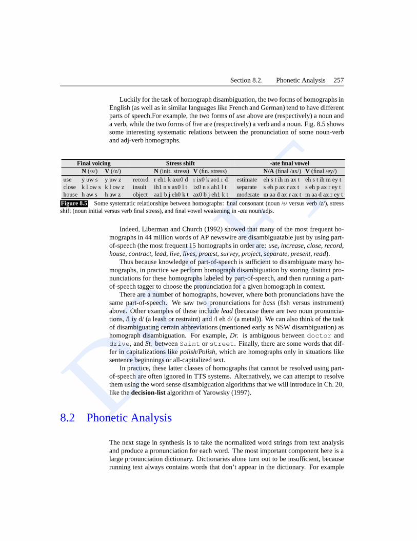
Luckily for the task of homograph disambiguation, the two forms of homographs inEnglish (as well as in similar languages like French and German) tend to have differentparts of speech.For example, the two forms ofuseabove are (respectively) a noun anda verb, while the two forms oflive are (respectively) a verb and a noun. Fig. 8.5 showssome interesting systematic relations between the pronunciation of some noun-verband adj-verb homographs.
Final voicing Stress shift -ate final vowelN (/s/) V (/z/) N (init. stress) V (fin. stress) N/A (final /ax/) V (final /ey/)
use y uw s y uw z record r eh1 k axr0 d r ix0 k ao1 r d estimate eh s t ih m ax t eh s t ih m ey tclose k l ow s k l ow z insult ih1 n s ax0 l t ix0 n s ah1 l t separate s eh p ax r ax t s eh p ax r ey thouse h aw s h aw z object aa1 b j eh0 k t ax0 b j eh1 k t moderate m aa d ax r ax tm aa d ax r ey t
Figure 8.5 Some systematic relationships between homographs: final consonant (noun /s/ versus verb /z/), stressshift (noun initial versus verb final stress), and final vowelweakening in-atenoun/adjs.
Indeed, Liberman and Church (1992) showed that many of the most frequent ho-mographs in 44 million words of AP newswire are disambiguatable just by using part-of-speech (the most frequent 15 homographs in order are:use, increase, close, record,house, contract, lead, live, lives, protest, survey, project, separate, present, read).
Thus because knowledge of part-of-speech is sufficient to disambiguate many ho-mographs, in practice we perform homograph disambiguationby storing distinct pro-nunciations for these homographs labeled by part-of-speech, and then running a part-of-speech tagger to choose the pronunciation for a given homograph in context.
There are a number of homographs, however, where both pronunciations have thesame part-of-speech. We saw two pronunciations forbass(fish versus instrument)above. Other examples of these includelead (because there are two noun pronuncia-tions, /l iy d/ (a leash or restraint) and /l eh d/ (a metal)). We can also think of the taskof disambiguating certain abbreviations (mentioned earlyas NSW disambiguation) ashomograph disambiguation. For example,Dr. is ambiguous betweendoctor anddrive , andSt. betweenSaint or street . Finally, there are some words that dif-fer in capitalizations likepolish/Polish, which are homographs only in situations likesentence beginnings or all-capitalized text.
In practice, these latter classes of homographs that cannotbe resolved using part-of-speech are often ignored in TTS systems. Alternatively,we can attempt to resolvethem using the word sense disambiguation algorithms that wewill introduce in Ch. 20,like thedecision-listalgorithm of Yarowsky (1997).
8.2 Phonetic Analysis
The next stage in synthesis is to take the normalized word strings from text analysisand produce a pronunciation for each word. The most important component here is alarge pronunciation dictionary. Dictionaries alone turn out to be insufficient, becauserunning text always contains words that don’t appear in the dictionary. For example
DRAFT
258 Chapter 8. Speech Synthesis
Black et al. (1998) used a British English dictionary, the OALD lexicon on the firstsection of the Penn Wall Street Journal Treebank. Of the 39923 words (tokens) in thissection, 1775 word tokens (4.6%) were not in the dictionary,of which 943 are unique(i.e. 943 types). The distributions of these unseen word tokens was as follows:
names unknown typos and other1360 351 6476.6% 19.8% 3.6%
Thus the two main areas where dictionaries need to be augmented is in dealing withnames and with other unknown words. We’ll discuss dictionaries in the next section,followed by names, and then turn to grapheme-to-phoneme rules for dealing with otherunknown words.
8.2.1 Dictionary Lookup
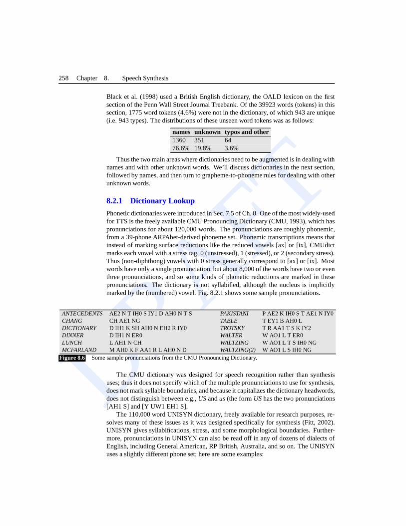
Phonetic dictionaries were introduced in Sec. 7.5 of Ch. 8. One of the most widely-usedfor TTS is the freely available CMU Pronouncing Dictionary (CMU, 1993), which haspronunciations for about 120,000 words. The pronunciations are roughly phonemic,from a 39-phone ARPAbet-derived phoneme set. Phonemic transcriptions means thatinstead of marking surface reductions like the reduced vowels [ax] or [ix], CMUdictmarks each vowel with a stress tag, 0 (unstressed), 1 (stressed), or 2 (secondary stress).Thus (non-diphthong) vowels with 0 stress generally correspond to [ax] or [ix]. Mostwords have only a single pronunciation, but about 8,000 of the words have two or eventhree pronunciations, and so some kinds of phonetic reductions are marked in thesepronunciations. The dictionary is not syllabified, although the nucleus is implicitlymarked by the (numbered) vowel. Fig. 8.2.1 shows some samplepronunciations.
ANTECEDENTS AE2 N T IH0 S IY1 D AH0 N T S PAKISTANI P AE2 K IH0 S T AE1 N IY0CHANG CH AE1 NG TABLE T EY1 B AH0 LDICTIONARY D IH1 K SH AH0 N EH2 R IY0 TROTSKY T R AA1 T S K IY2DINNER D IH1 N ER0 WALTER W AO1 L T ER0LUNCH L AH1 N CH WALTZING W AO1 L T S IH0 NGMCFARLAND M AH0 K F AA1 R L AH0 N D WALTZING(2) W AO1 L S IH0 NG
Figure 8.6 Some sample pronunciations from the CMU Pronouncing Dictionary.
The CMU dictionary was designed for speech recognition rather than synthesisuses; thus it does not specify which of the multiple pronunciations to use for synthesis,does not mark syllable boundaries, and because it capitalizes the dictionary headwords,does not distinguish between e.g.,USandus(the formUShas the two pronunciations[AH1 S] and [Y UW1 EH1 S].
The 110,000 word UNISYN dictionary, freely available for research purposes, re-solves many of these issues as it was designed specifically for synthesis (Fitt, 2002).UNISYN gives syllabifications, stress, and some morphological boundaries. Further-more, pronunciations in UNISYN can also be read off in any of dozens of dialects ofEnglish, including General American, RP British, Australia, and so on. The UNISYNuses a slightly different phone set; here are some examples:
DRAFT
Section 8.2. Phonetic Analysis 259
going: { g * ou }.> i ng >antecedents: { * a n . tˆ i . s ˜ ii . d n! t }> s >dictionary: { d * i k . sh @ . n ˜ e . r ii }
8.2.2 Names
As the error analysis above indicated, names are an important issue in speech synthe-sis. The many types can be categorized into personal names (first names and surnames),geographical names (city, street, and other place names), and commercial names (com-pany and product names). For personal names alone, Spiegel (2003) gives an estimatefrom Donnelly and other household lists of about two milliondifferent surnames and100,000 first names just for the United States. Two million isa very large number; anorder of magnitude more than the entire size of the CMU dictionary. For this reason,most large-scale TTS systems include a large name pronunciation dictionary. As wesaw in Fig. 8.2.1 the CMU dictionary itself contains a wide variety of names; in partic-ular it includes the pronunciations of the most frequent 50,000 surnames from an oldBell Lab estimate of US personal name frequency, as well as 6,000 first names.
How many names are sufficient? Liberman and Church (1992) found that a dic-tionary of 50,000 names covered 70% of the name tokens in 44 million words of APnewswire. Interestingly, many of the remaining names (up to97.43% of the tokens intheir corpus) could be accounted for by simple modificationsof these 50,000 names.For example, some name pronunciations can be created by adding simple stress-neutralsuffixes likes or ville to names in the 50,000, producing new names as follows:
walters = walter+s lucasville = lucas+ville abelson = abel+ son
Other pronunciations might be created by rhyme analogy. If we have the pronunci-ation for the nameTrotsky, but not the namePlotsky, we can replace the initial /tr/ fromTrotskywith initial /pl/ to derive a pronunciation forPlotsky.
Techniques such as this, including morphological decomposition, analogical for-mation, and mapping unseen names to spelling variants already in the dictionary (Fack-rell and Skut, 2004), have achieved some success in name pronunciation. In general,however, name pronunciation is still difficult. Many modernsystems deal with un-known names via the grapheme-to-phoneme methods describedin the next section, of-ten by building two predictive systems, one for names and onefor non-names. Spiegel(2003, 2002) summarizes many more issues in proper name pronunciation.
8.2.3 Grapheme-to-Phoneme
Once we have expanded non-standard words and looked them allup in a pronuncia-tion dictionary, we need to pronounce the remaining, unknown words. The processof converting a sequence of letters into a sequence of phonesis calledgrapheme-to-phonemeconversion, sometimes shortenedg2p. The job of a grapheme-to-phonemeGrapheme-to-
phonemealgorithm is thus to convert a letter string likecakeinto a phone string like[K EY K] .
DRAFT
260 Chapter 8. Speech Synthesis
The earliest algorithms for grapheme-to-phoneme conversion were rules written byhand using the Chomsky-Halle phonological rewrite rule format of Eq. 7.1 in Ch. 7.These are often calledletter-to-sound or LTS rules, and they are still used in someLetter-to-sound
systems. LTS rules are applied in order, with later (default) rules only applying if thecontext for earlier rules are not applicable. A simple pair of rules for pronouncing theletterc might be as follows:
c → [k] / {a,o}V ; context-dependent(8.11)
c → [s] ; context-independent(8.12)
Actual rules must be much more complicated (for examplec can also be pro-nounced [ch] incello or concerto). Even more complex are rules for assigning stress,which are famously difficult for English. Consider just one of the many stress rulesfrom Allen et al. (1987), where the symbolX represents all possible syllable onsets:
(8.13) V→ [+stress] /X C* {VshortC C?|V} {VshortC*|V}This rule represents the following two situations:
1. Assign 1-stress to the vowel in a syllable preceding a weaksyllable followed by a morpheme-final syllable containing a short vowel and 0 or more consonants (e.g.difficult)
2. Assign 1-stress to the vowel in a syllable preceding a weaksyllable followed by a morpheme-final vowel (e.g.oregano)
While some modern systems still use such complex hand-written rules, most sys-tems achieve higher accuracy by relying instead on automatic or semi-automatic meth-ods based on machine learning. This modern probabilistic grapheme-to-phonemeprob-lem was first formalized by Lucassen and Mercer (1984). Givena letter sequenceL,we are searching for the most probable phone sequenceP:
P = argmaxP
P(P|L)(8.14)
The probabilistic method assumes a training set and a test set; both sets are lists ofwords from a dictionary, with a spelling and a pronunciationfor each word. The nextsubsections show how the populardecision treemodel for estimating this probabilityP(P|L) can be trained and applied to produce the pronunciation for an unseen word.
Finding a letter-to-phone alignment for the training set
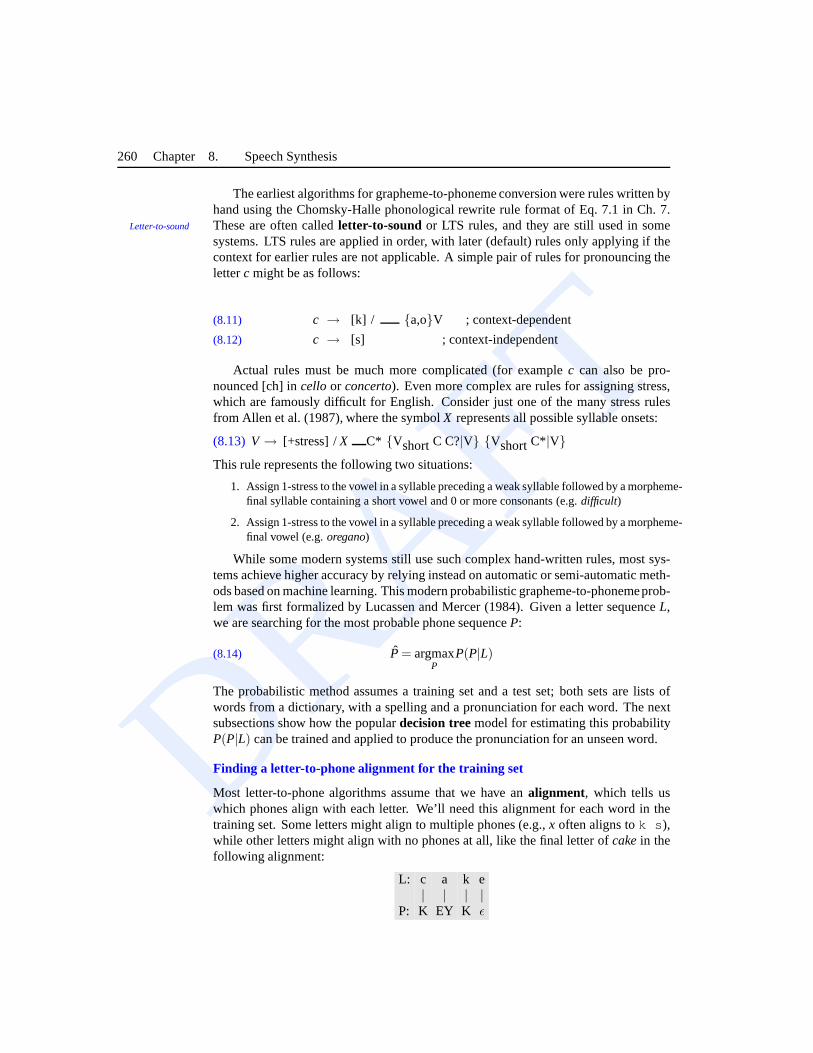
Most letter-to-phone algorithms assume that we have analignment, which tells uswhich phones align with each letter. We’ll need this alignment for each word in thetraining set. Some letters might align to multiple phones (e.g.,x often aligns tok s ),while other letters might align with no phones at all, like the final letter ofcakein thefollowing alignment:
L: c a k e| | | |
P: K EY K ǫ
DRAFT
Section 8.2. Phonetic Analysis 261
One method for finding such a letter-to-phone alignment is the semi-automaticmethod of (Black et al., 1998). Their algorithm is semi-automatic because it relieson a hand-written list of theallowable phones that can realize each letter. Here areallowables lists for the lettersc ande:
c: k ch s sh t-s ǫe: ih iy er ax ah eh ey uw ay ow y-uw oy aa ǫ
In order to produce an alignment for each word in the trainingset, we take thisallowables list for all the letters, and for each word in the training set, we find allalignments between the pronunciation and the spelling thatconform to the allowableslist. From this large list of alignments, we compute, by summing over all alignmentsfor all words, the total count for each letter being aligned to each phone (or multi-phone orǫ). From these counts we can normalize to get for each phonepi and letterl j
a probabilityP(pi |l j):
P(pi |l j) =count(pi , l j)
count(l j )(8.15)
We can now take these probabilities and realign the letters to the phones, usingthe Viterbi algorithm to produce the best (Viterbi) alignment for each word, wherethe probability of each alignment is just the product of all the individual phone/letteralignments.
In this way we can produce a single good alignmentA for each particular pair(P,L)in our training set.
Choosing the best phone string for the test set
Given a new wordw, we now need to map its letters into a phone string. To do this,we’ll first train a machine learning classifier, like a decision tree, on the aligned trainingset. The job of the classifier will be to look at a letter of the word and generate the mostprobable phone.
What features should we use in this decision tree besides thealigned letterl i itself?Obviously we can do a better job of predicting the phone if we look at a windowof surrounding letters; for example consider the lettera. In the wordcat, the a ispronounceAE. But in our wordcake, a is pronouncedEY, becausecakehas a finale;thus knowing whether there is a finale is a useful feature. Typically we look at thekprevious letters and thek following letters.
Another useful feature would be the correct identity of the previous phone. Know-ing this would allow us to get some phonotactic information into our probability model.Of course, we can’t know the true identity of the previous phone, but we can approxi-mate this by looking at the previous phone that was predictedby our model. In order todo this, we’ll need to run our decision tree left to right, generating phones one by one.
In summary, in the most common decision tree model, the probability of each phonepi is estimated from a window ofk previous andk following letters, as well as the mostrecentk phones that were previously produced.
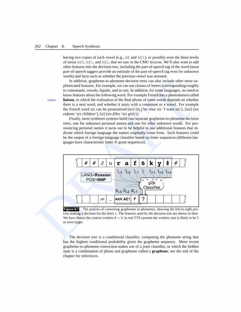
Fig. 8.7 shows a sketch of this left-to-right process, indicating the features that adecision tree would use to decide the letter corresponding to the letters in the wordJurafsky. As this figure indicates, we can integrate stress prediction into phone pre-diction by augmenting our set of phones with stress information. We can do this by
DRAFT
262 Chapter 8. Speech Synthesis
having two copies of each vowel (e.g.,AEandAE1), or possibly even the three levelsof stressAE0, AE1, andAE2, that we saw in the CMU lexicon. We’ll also want to addother features into the decision tree, including the part-of-speech tag of the word (mostpart-of-speech taggers provide an estimate of the part-of-speech tag even for unknownwords) and facts such as whether the previous vowel was stressed.
In addition, grapheme-to-phoneme decision trees can also include other more so-phisticated features. For example, we can use classes of letters (corresponding roughlyto consonants, vowels, liquids, and so on). In addition, forsome languages, we need toknow features about the following word. For example French has a phenomenon calledliaison, in which the realization of the final phone of some words depends on whetherLiaison
there is a next word, and whether it starts with a consonant ora vowel. For examplethe French wordsix can be pronounced [sis] (inj’en veux six‘I want six’), [siz] (sixenfants‘six children’), [si] (six filles‘six girls’).
Finally, most synthesis systems build two separate grapheme-to-phoneme decisiontrees, one for unknown personal names and one for other unknown words. For pro-nouncing personal names it turns out to be helpful to use additional features that in-dicate which foreign language the names originally come from. Such features couldbe the output of a foreign-language classifier based on letter sequences (different lan-guages have characteristic letterN-gram sequences).
# # J u r a f s k y # #
56 _ AXR AE1 F ?
g2p Classifier
a
li-3 li-2 li-1
pi-3 pi-2 pi-1
LANG=RussianPOS=NNP
li li+1 li+2 li+3
Figure 8.7 The process of converting graphemes to phonemes, showing the left-to-right pro-cess making a decision for the letters. The features used by the decision tree are shown in blue.We have shown the context windowk = 3; in real TTS systems the window size is likely to be 5or even larger.
The decision tree is a conditional classifier, computing thephoneme string thathas the highest conditional probability given the graphemesequence. More recentgrapheme-to-phoneme conversion makes use of a joint classifier, in which the hiddenstate is a combination of phone and grapheme called agraphone; see the end of thechapter for references.
DRAFT
Section 8.3. Prosodic Analysis 263
8.3 Prosodic Analysis
The final stage of linguistic analysis is prosodic analysis.In poetry, the wordprosodyProsody
refers to the study of the metrical structure of verse. In linguistics and language pro-cessing, however, we use the termprosody to mean the study of the intonational andrhythmic aspects of language. More technically, prosody has been defined by Ladd(1996) as the ‘use of suprasegmental features to convey sentence-level pragmatic mean-ings’. The termsuprasegmentalmeans above and beyond the level of the segment orSuprasegmental
phone, and refers especially to the uses of acoustic features like F0 duration, andenergy independently of the phone string.
By sentence-level pragmatic meaning, Ladd is referring to a number of kindsof meaning that have to do with the relation between a sentence and its discourseor external context. For example, prosody can be used to markdiscourse structureor function , like the difference between statements and questions, or the way that aconversation is structured into segments or subdialogs. Prosody is also used to marksaliency, such as indicating that a particular word or phrase is important or salient. Fi-nally, prosody is heavily used for affective and emotional meaning, such as expressinghappiness, surprise, or anger.
In the next sections we will introduce the three aspects of prosody, each of which isimportant for speech synthesis:prosodic prominence, prosodic structure andtune.Prosodic analysis generally proceeds in two parts. First, we compute an abstract repre-sentation of the prosodic prominence, structure and tune ofthe text. For unit selectionsynthesis, this is all we need to do in the text analysis component. For diphone andHMM synthesis, we have one further step, which is to predictduration andF0 valuesfrom these prosodic structures.
8.3.1 Prosodic Structure
Spoken sentences have prosodic structure in the sense that some words seem to groupnaturally together and some words seem to have a noticeable break or disjuncture be-tween them. Often prosodic structure is described in terms of prosodic phrasing,Prosodic Phrasing
meaning that an utterance has a prosodic phrase structure ina similar way to it havinga syntactic phrase structure. For example, in the sentenceI wanted to go to London, butcould only get tickets for Francethere seems to be two mainintonation phrases, theirIntonation phrase
boundary occurring at the comma. Furthermore, in the first phrase, there seems to beanother set of lesser prosodic phrase boundaries (often called intermediate phrases)intermediate
phrase
that split up the words as followsI wanted| to go| to London.Prosodic phrasing has many implications for speech synthesis; the final vowel of a
phrase is longer than usual, we often insert a pause after an intonation phrases, and, aswe will discuss in Sec. 8.3.6, there is often a slight drop in F0 from the beginning of anintonation phrase to its end, which resets at the beginning of a new intonation phrase.
Practical phrase boundary prediction is generally treatedas a binary classificationtask, where we are given a word and we have to decide whether ornot to put a prosodicboundary after it. A simple model for boundary prediction can be based on determinis-tic rules. A very high-precision rule is the one we saw for sentence segmentation: insert
DRAFT
264 Chapter 8. Speech Synthesis
a boundary after punctuation. Another commonly used rule inserts a phrase boundarybefore a function word following a content word.
More sophisticated models are based on machine learning classifiers. To createa training set for classifiers, we first choose a corpus, and then mark every prosodicboundaries in the corpus. One way to do this prosodic boundary labeling is to usean intonational model like ToBI or Tilt (see Sec. 8.3.4), have human labelers listen tospeech and label the transcript with the boundary events defined by the theory. Becauseprosodic labeling is extremely time-consuming, however, atext-only alternative is of-ten used. In this method, a human labeler looks only at the text of the training corpus,ignoring the speech. The labeler marks any juncture betweenwords where they feel aprosodic boundary might legitimately occur if the utterance were spoken.
Given a labeled training corpus, we can train a decision treeor other classifier tomake a binary (boundary vs. no boundary) decision at every juncture between words(Wang and Hirschberg, 1992; Ostendorf and Veilleux, 1994; Taylor and Black, 1998).
Features that are commonly used in classification include:
• Length features: phrases tend to be of roughly equal length, and so we canuse various feature that hint at phrase length (Bachenko andFitzpatrick, 1990;Grosjean et al., 1979; Gee and Grosjean, 1983).
– The total number of words and syllables in utterance– The distance of the juncture from the beginning and end of thesentence (in
words or syllables)– The distance in words from the last punctuation mark
• Neighboring part-of-speech and punctuation:
– The part-of-speech tags for a window of words around the juncture. Gen-erally the two words before and after the juncture are used.
– The type of following punctuation
There is also a correlation between prosodic structure and thesyntactic structurethat will be introduced in Ch. 12, Ch. 13, and Ch. 14 (Price et al., 1991). Thus robustparsers like Collins (1997) can be used to label the sentencewith rough syntactic in-formation, from which we can extract syntactic features such as the size of the biggestsyntactic phrase that ends with this word (Ostendorf and Veilleux, 1994; Koehn et al.,2000).
8.3.2 Prosodic prominence
In any spoken utterance, some words sound moreprominent than others. ProminentProminence
words are perceptually more salient to the listener; speakers make a word more salientin English by saying it louder, saying it slower (so it has a longer duration), or byvarying F0 during the word, making it higher or more variable.
We generally capture the core notion of prominence by associating a linguisticmarker with prominent words, a marker calledpitch accent. Words which are promi-Pitch accent
nent are said tobear (be associated with) a pitch accent. Pitch accent is thus part of thephonological description of a word in context in a spoken utterance.
Pitch accent is related tostress, which we discussed in Ch. 7. The stressed syllableof a word is where pitch accent is realized. In other words, ifa speaker decides to
DRAFT
Section 8.3. Prosodic Analysis 265
highlight a word by giving it a pitch accent, the accent will appear on the stressedsyllable of the word.
The following example shows accented words in capital letters, with the stressedsyllable bearing the accent (the louder, longer, syllable)in boldface:
(8.16) I’m a little SURPRISED to hear itCHARACTERIZED as UPBEAT .
Note that the function words tend not to bear pitch accent, while most of the contentwords are accented. This is a special case of the more generalfact that very informativewords (content words, and especially those that are new or unexpected) tend to bearaccent (Ladd, 1996; Bolinger, 1972).
We’ve talked so far as if we only need to make a binary distinction between ac-cented and unaccented words. In fact we generally need to make more fine-graineddistinctions. For example the last accent in a phrase generally is perceived as beingmore prominent than the other accents. This prominent last accent is called thenu-clear accent. Emphatic accents like nuclear accent are generally used for semanticNuclear accent
purposes, for example to indicate that a word is thesemantic focusof the sentence(see Ch. 21) or that a word is contrastive or otherwise important in some way. Suchemphatic words are the kind that are often written IN CAPITALLETTERS or with**STARS** around them in SMS or email orAlice in Wonderland; here’s an examplefrom the latter:
(8.17) ‘I know SOMETHING interesting is sure to happen,’ she said toherself,
Another way that accent can be more complex than just binary is that some wordscan belessprominent than usual. We introduced in Ch. 7 the idea that function wordsare often phonetically veryreduced.
A final complication is that accents can differ according to thetune associated withthem; for example accents with particularly high pitch havedifferent functions thanthose with particularly low pitch; we’ll see how this is modeled in the ToBI model inSec. 8.3.4.
Ignoring tune for the moment, we can summarize by saying thatspeech synthesissystems can use as many as four levels of prominence:emphatic accent, pitch accent,unaccented, andreduced. In practice, however, many implemented systems make dowith a subset of only two or three of these levels.
Let’s see how a 2-level system would work. With two-levels, pitch accent predic-tion is a binary classification task, where we are given a wordand we have to decidewhether it is accented or not.
Since content words are very often accented, and function words are very rarelyaccented, the simplest accent prediction system is just to accent all content words andno function words. In most cases better models are necessary.
In principle accent prediction requires sophisticated semantic knowledge, for ex-ample to understand if a word is new or old in the discourse, whether it is being usedcontrastively, and how much new information a word contains. Early models made useof sophisticated linguistic models of all of this information (Hirschberg, 1993). ButHirschberg and others showed better prediction by using simple, robust features thatcorrelate with these sophisticated semantics.
For example, the fact that new or unpredictable informationtends to be accentedcan be modeled by using robust features likeN-grams or TF*IDF (Pan and Hirschberg,
DRAFT
266 Chapter 8. Speech Synthesis
2000; Pan and McKeown, 1999). The unigram probability of a word P(wi) and itsbigram probabilityP(wi |wi−1), both correlate with accent; the more probable a word,the less likely it is to be accented. Similarly, an information-retrieval measure known asTF*IDF (Term-Frequency/Inverse-DocumentFrequency; see Ch. 23)is a useful accentTF*IDF
predictor. TF*IDF captures the semantic importance of a word in a particular documentd, by downgrading words that tend to appear in lots of different documents in somelarge background corpus withN documents. There are various versions of TF*IDF;one version can be expressed formally as follows, assumingNw is the frequency ofwin the documentd, andk is the total number of documents in the corpus that containw:
TF*IDF(w) = Nw× log(Nk
)(8.18)
For words which have been seen enough times in a training set,the accent ratioAccent ratio
feature can be used, which models a word’s individual probability of being accented.The accent ratio of a word is equal to the estimated probability of the word being ac-cented if this probability is significantly different from 0.5, and equal to 0.5 otherwise.More formally,
AccentRatio(w) =
{kN if B(k,N,0.5)≤ 0.05
0.5 otherwise
whereN is the total number of times the wordw occurred in the training set,k is thenumber of times it was accented, andB(k,n,0.5) is the probability (under a binomialdistribution) that there arek successes inn trials if the probability of success and failureis equal (Nenkova et al., 2007; Yuan et al., 2005).
Features like part-of-speech,N-grams, TF*IDF, and accent ratio can then be com-bined in a decision tree to predict accents. While these robust features work relativelywell, a number of problems in accent prediction still remainthe subject of research.
For example, it is difficult to predict which of the two words should be accentedin adjective-noun or noun-noun compounds. Some regularities do exist; for exampleadjective-noun combinations likenew truckare likely to have accent on the right word(new TRUCK), while noun-noun compounds likeTREE surgeonare likely to have ac-cent on the left. But the many exceptions to these rules make accent prediction in nouncompounds quite complex. For example the noun-noun compound APPLE cakehasthe accent on the first word while the noun-noun compoundapple PIEor city HALLboth have the accent on the second word (Liberman and Sproat,1992; Sproat, 1994,1998a).
Another complication has to do with rhythm; in general speakers avoid puttingaccents too close together (a phenomenon known asclash) or too far apart (lapse).Clash
Lapse Thuscity HALLandPARKING lotcombine asCITY hall PARKING lotwith the accenton HALL shifting forward toCITY to avoid the clash with the accent onPARKING(Liberman and Prince, 1977),
Some of these rhythmic constraints can be modeled by using machine learningtechniques that are more appropriate for sequence modeling. This can be done byrunning a decision tree classifier left to right through a sentence, and using the outputof the previous word as a feature, or by using more sophisticated machine learningmodels like Conditional Random Fields (CRFs) (Gregory and Altun, 2004).
DRAFT
Section 8.3. Prosodic Analysis 267
8.3.3 Tune
Two utterances with the same prominence and phrasing patterns can still differ prosod-ically by having differenttunes. The tune of an utterance is the rise and fall of itsTune
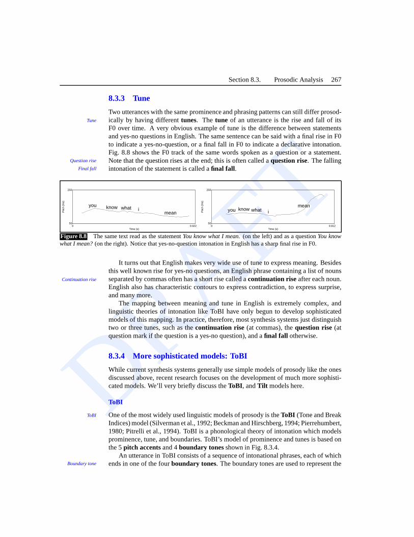
F0 over time. A very obvious example of tune is the differencebetween statementsand yes-no questions in English. The same sentence can be said with a final rise in F0to indicate a yes-no-question, or a final fall in F0 to indicate a declarative intonation.Fig. 8.8 shows the F0 track of the same words spoken as a question or a statement.Note that the question rises at the end; this is often called aquestion rise. The fallingQuestion rise
intonation of the statement is called afinal fall .Final fall
Time (s)0 0.922
Pitc
h (H
z)
50
250
you know what imean
Time (s)0 0.912
Pitc
h (H
z)
50
250
you know what imean
Figure 8.8 The same text read as the statementYou know what I mean. (on the left) and as a questionYou knowwhat I mean?(on the right). Notice that yes-no-question intonation in English has a sharp final rise in F0.
It turns out that English makes very wide use of tune to express meaning. Besidesthis well known rise for yes-no questions, an English phrasecontaining a list of nounsseparated by commas often has a short rise called acontinuation rise after each noun.Continuation rise
English also has characteristic contours to express contradiction, to express surprise,and many more.
The mapping between meaning and tune in English is extremelycomplex, andlinguistic theories of intonation like ToBI have only begunto develop sophisticatedmodels of this mapping. In practice, therefore, most synthesis systems just distinguishtwo or three tunes, such as thecontinuation rise (at commas), thequestion rise (atquestion mark if the question is a yes-no question), and afinal fall otherwise.
8.3.4 More sophisticated models: ToBI
While current synthesis systems generally use simple models of prosody like the onesdiscussed above, recent research focuses on the development of much more sophisti-cated models. We’ll very briefly discuss theToBI , andTilt models here.
ToBI
One of the most widely used linguistic models of prosody is theToBI (Tone and BreakToBI
Indices) model (Silverman et al., 1992; Beckman and Hirschberg, 1994; Pierrehumbert,1980; Pitrelli et al., 1994). ToBI is a phonological theory of intonation which modelsprominence, tune, and boundaries. ToBI’s model of prominence and tunes is based onthe 5pitch accentsand 4boundary tonesshown in Fig. 8.3.4.
An utterance in ToBI consists of a sequence of intonational phrases, each of whichends in one of the fourboundary tones. The boundary tones are used to represent theBoundary tone
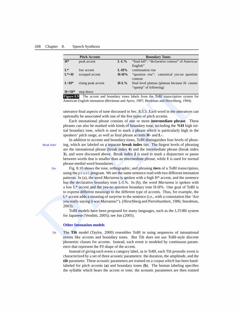
DRAFT
268 Chapter 8. Speech Synthesis
Pitch Accents Boundary TonesH* peak accent L-L% “final fall”: “declarative contour” of American
English”L* low accent L-H% continuation riseL*+H scooped accent H-H% “question rise”: cantonical yes-no question
contourL+H* rising peak accent H-L% final level plateau (plateau because H- causes
“upstep” of following)H+!H* step down
Figure 8.9 The accent and boundary tones labels from the ToBI transcription system forAmerican English intonation (Beckman and Ayers, 1997; Beckman and Hirschberg, 1994).
utterance final aspects of tune discussed in Sec. 8.3.3. Eachword in the utterances canoptionally be associated with one of the five types of pitch accents.
Each intonational phrase consists of one or moreintermediate phrase. Thesephrases can also be marked with kinds of boundary tone, including the%H high ini-tial boundary tone, which is used to mark a phrase which is particularly high in thespeakers’ pitch range, as well as final phrase accentsH- andL- .
In addition to accents and boundary tones, ToBI distinguishes four levels of phras-ing, which are labeled on a separatebreak index tier. The largest levels of phrasingBreak index
are the intonational phrase (break index4) and the intermediate phrase (break index3), and were discussed above. Break index2 is used to mark a disjuncture or pausebetween words that is smaller than an intermediate phrase, while 1 is used for normalphrase-medial word boundaries.
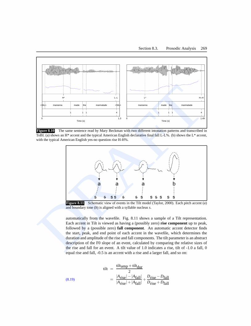
Fig. 8.10 shows the tone, orthographic, and phrasingtiers of a ToBI transcription,Tier
using thepraat program. We see the same sentence read with two different intonationpatterns. In (a), the wordMarianna is spoken with a high H* accent, and the sentencehas the declarative boundary tone L-L%. In (b), the wordMarianna is spoken witha low L* accent and the yes-no question boundary tone H-H%. One goal of ToBI isto express different meanings to the different type of accents. Thus, for example, theL* accent adds a meaning ofsurpriseto the sentence (i.e., with a connotation like ‘Areyou really saying it was Marianna?’). (Hirschberg and Pierrehumbert, 1986; Steedman,2003).
ToBI models have been proposed for many languages, such as the J TOBI systemfor Japanese (Venditti, 2005); see Jun (2005).
Other Intonation models
The Tilt model (Taylor, 2000) resembles ToBI in using sequences of intonationalTilt
events like accents and boundary tones. But Tilt does not useToBI-style discretephonemic classes for accents. Instead, each event is modeled by continuous param-eters that represent the F0 shape of the accent.
Instead of giving each event a category label, as in ToBI, each Tilt prosodic event ischaracterized by a set of three acoustic parameters: the duration, the amplitude, and thetilt parameter. These acoustic parameters are trained on a corpus which has been hand-labeled for pitch accents (a) and boundary tones (b). The human labeling specifiesthe syllable which bears the accent or tone; the acoustic parameters are then trained
DRAFT
Section 8.3. Prosodic Analysis 269
H* L–L
<SIL> marianna made the marmalade <SIL>
1 1 1 4
Time (s)0 1.3
L* H–H
marianna made the marmalade
1 1 1 4
Time (s)0 1.49
Figure 8.10 The same sentence read by Mary Beckman with two different intonation patterns and transcribed inToBI. (a) shows an H* accent and the typical American Englishdeclarative final fall L-L%. (b) shows the L* accent,with the typical American English yes-no question rise H-H%.
a a a b7 7 7 7 7 7 7 7 7 7 7 7Figure 8.11 Schematic view of events in the Tilt model (Taylor, 2000). Each pitch accent (a)and boundary tone (b) is aligned with a syllable nucleuss.
automatically from the wavefile. Fig. 8.11 shows a sample of aTilt representation.Each accent in Tilt is viewed as having a (possibly zero)rise componentup to peak,followed by a (possible zero)fall component. An automatic accent detector findsthe start, peak, and end point of each accent in the wavefile, which determines theduration and amplitude of the rise and fall components. The tilt parameter is an abstractdescription of the F0 slope of an event, calculated by comparing the relative sizes ofthe rise and fall for an event. A tilt value of 1.0 indicates a rise, tilt of -1.0 a fall, 0equal rise and fall, -0.5 is an accent with a rise and a larger fall, and so on:
tilt =tilt amp+ tiltdur
2
=|Arise|− |Afall||Arise|+ |Afall|
+Drise−DfallDrise+Dfall
(8.19)
DRAFT
270 Chapter 8. Speech Synthesis
See the end of the chapter for pointers to other intonationalmodels.
8.3.5 Computing duration from prosodic labels
The results of the text analysis processes described so far is a string of phonemes,annotated with words, with pitch accent marked on relevant words, and appropriateboundary tones marked. For theunit selectionsynthesis approaches that we will de-scribe in Sec. 8.5, this is a sufficient output from the text analysis component.
Fordiphone synthesis, as well as other approaches like formant synthesis, we alsoneed to specify theduration and theF0 values of each segment.
Phones vary quite a bit in duration. Some of the duration is inherent to the identityof the phone itself. Vowels, for example, are generally muchlonger than consonants;in the Switchboard corpus of telephone speech, the phone [aa] averages 118 millisec-onds, while [d] averages 68 milliseconds. But phone duration is also affected by awide variety of contextual factors, which can be modeled by rule-based or statisticalmethods.
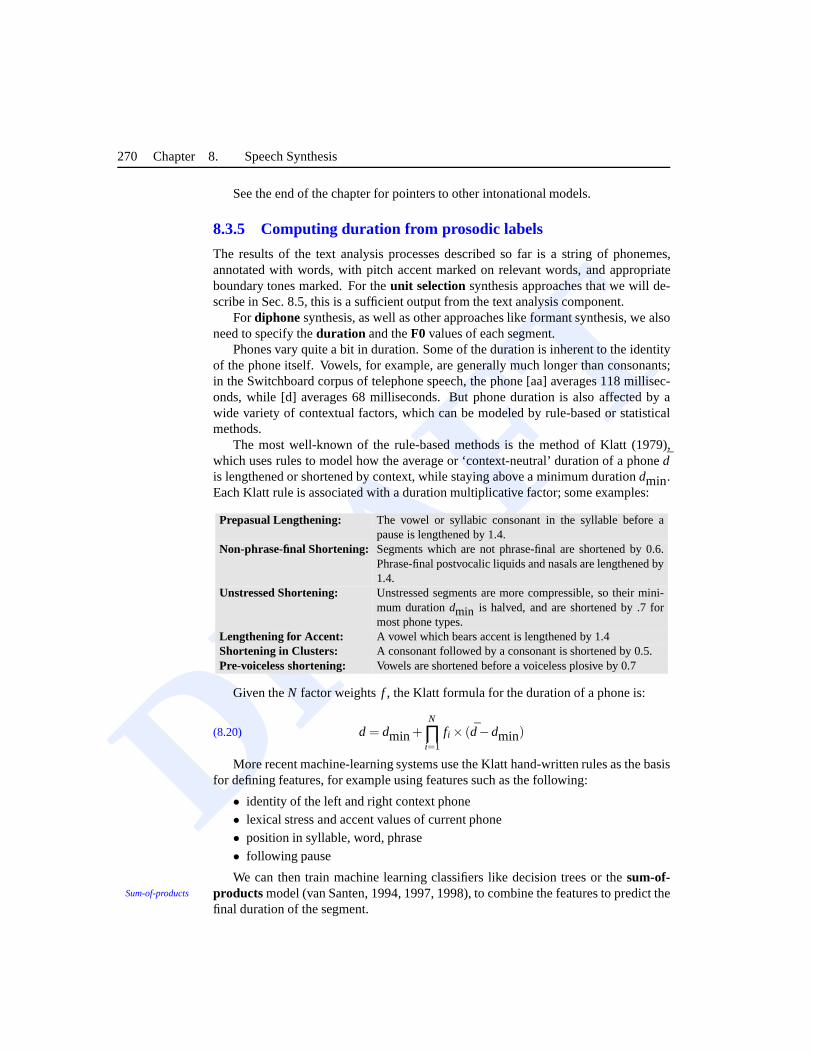
The most well-known of the rule-based methods is the method of Klatt (1979),which uses rules to model how the average or ‘context-neutral’ duration of a phonedis lengthened or shortened by context, while staying above aminimum durationdmin.Each Klatt rule is associated with a duration multiplicative factor; some examples:
Prepasual Lengthening: The vowel or syllabic consonant in the syllable before apause is lengthened by 1.4.
Non-phrase-final Shortening: Segments which are not phrase-final are shortened by 0.6.Phrase-final postvocalic liquids and nasals are lengthenedby1.4.
Unstressed Shortening: Unstressed segments are more compressible, so their mini-mum durationdmin is halved, and are shortened by .7 formost phone types.
Lengthening for Accent: A vowel which bears accent is lengthened by 1.4Shortening in Clusters: A consonant followed by a consonant is shortened by 0.5.Pre-voiceless shortening: Vowels are shortened before a voiceless plosive by 0.7
Given theN factor weightsf , the Klatt formula for the duration of a phone is:
d = dmin+N
∏i=1
fi × (d−dmin)(8.20)
More recent machine-learning systems use the Klatt hand-written rules as the basisfor defining features, for example using features such as thefollowing:
• identity of the left and right context phone• lexical stress and accent values of current phone• position in syllable, word, phrase• following pause
We can then train machine learning classifiers like decisiontrees or thesum-of-products model (van Santen, 1994, 1997, 1998), to combine the features to predict theSum-of-products
final duration of the segment.
DRAFT
Section 8.3. Prosodic Analysis 271
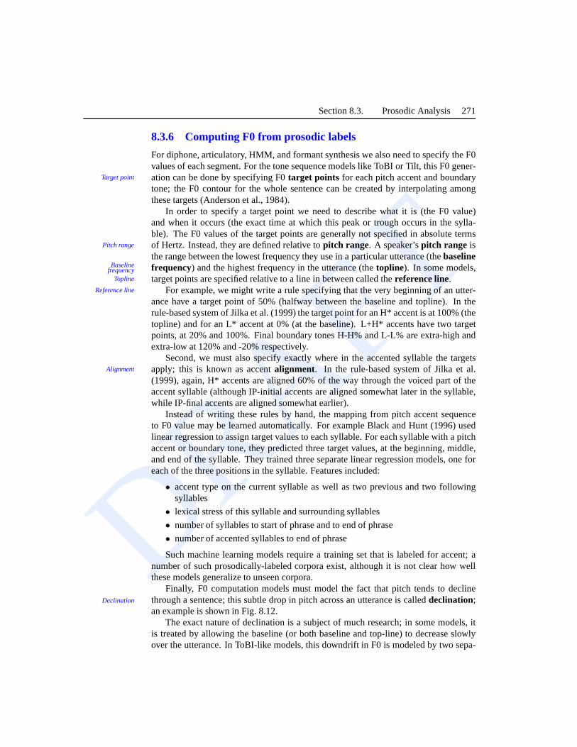
8.3.6 Computing F0 from prosodic labels
For diphone, articulatory, HMM, and formant synthesis we also need to specify the F0values of each segment. For the tone sequence models like ToBI or Tilt, this F0 gener-ation can be done by specifying F0target points for each pitch accent and boundaryTarget point
tone; the F0 contour for the whole sentence can be created by interpolating amongthese targets (Anderson et al., 1984).
In order to specify a target point we need to describe what it is (the F0 value)and when it occurs (the exact time at which this peak or troughoccurs in the sylla-ble). The F0 values of the target points are generally not specified in absolute termsof Hertz. Instead, they are defined relative topitch range. A speaker’spitch range isPitch range
the range between the lowest frequency they use in a particular utterance (thebaselinefrequency) and the highest frequency in the utterance (thetopline). In some models,Baseline
frequencyTopline target points are specified relative to a line in between called thereference line.
Reference line For example, we might write a rule specifying that the very beginning of an utter-ance have a target point of 50% (halfway between the baselineand topline). In therule-based system of Jilka et al. (1999) the target point foran H* accent is at 100% (thetopline) and for an L* accent at 0% (at the baseline). L+H* accents have two targetpoints, at 20% and 100%. Final boundary tones H-H% and L-L% are extra-high andextra-low at 120% and -20% respectively.
Second, we must also specify exactly where in the accented syllable the targetsapply; this is known as accentalignment. In the rule-based system of Jilka et al.Alignment
(1999), again, H* accents are aligned 60% of the way through the voiced part of theaccent syllable (although IP-initial accents are aligned somewhat later in the syllable,while IP-final accents are aligned somewhat earlier).
Instead of writing these rules by hand, the mapping from pitch accent sequenceto F0 value may be learned automatically. For example Black and Hunt (1996) usedlinear regression to assign target values to each syllable.For each syllable with a pitchaccent or boundary tone, they predicted three target values, at the beginning, middle,and end of the syllable. They trained three separate linear regression models, one foreach of the three positions in the syllable. Features included:
• accent type on the current syllable as well as two previous and two followingsyllables
• lexical stress of this syllable and surrounding syllables
• number of syllables to start of phrase and to end of phrase
• number of accented syllables to end of phrase
Such machine learning models require a training set that is labeled for accent; anumber of such prosodically-labeled corpora exist, although it is not clear how wellthese models generalize to unseen corpora.
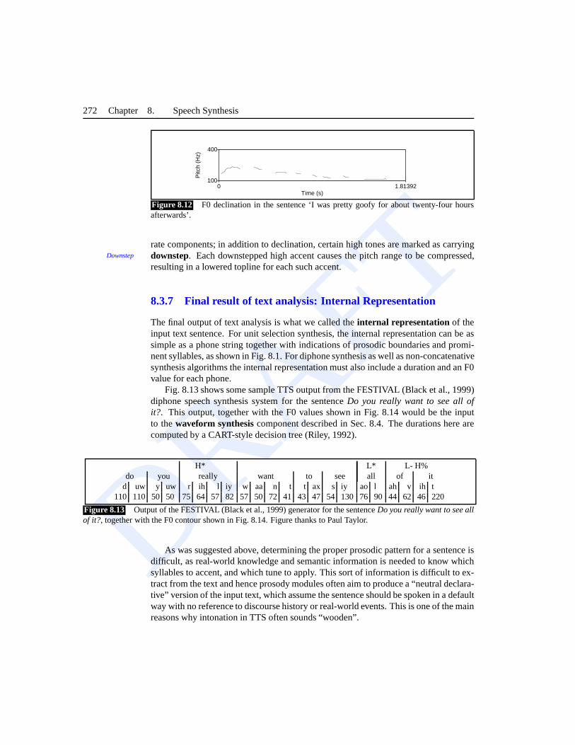
Finally, F0 computation models must model the fact that pitch tends to declinethrough a sentence; this subtle drop in pitch across an utterance is calleddeclination;Declination
an example is shown in Fig. 8.12.The exact nature of declination is a subject of much research; in some models, it
is treated by allowing the baseline (or both baseline and top-line) to decrease slowlyover the utterance. In ToBI-like models, this downdrift in F0 is modeled by two sepa-
DRAFT
272 Chapter 8. Speech Synthesis
Time (s)0 1.81392
Pitc
h (H
z)
100
400
Figure 8.12 F0 declination in the sentence ‘I was pretty goofy for about twenty-four hoursafterwards’.
rate components; in addition to declination, certain high tones are marked as carryingdownstep. Each downstepped high accent causes the pitch range to be compressed,Downstep
resulting in a lowered topline for each such accent.
8.3.7 Final result of text analysis: Internal Representation
The final output of text analysis is what we called theinternal representation of theinput text sentence. For unit selection synthesis, the internal representation can be assimple as a phone string together with indications of prosodic boundaries and promi-nent syllables, as shown in Fig. 8.1. For diphone synthesis as well as non-concatenativesynthesis algorithms the internal representation must also include a duration and an F0value for each phone.
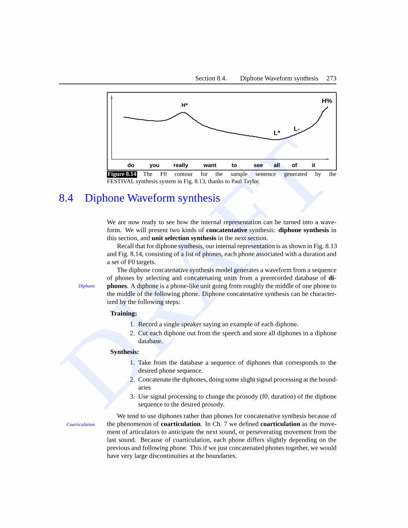
Fig. 8.13 shows some sample TTS output from the FESTIVAL (Black et al., 1999)diphone speech synthesis system for the sentenceDo you really want to see all ofit?. This output, together with the F0 values shown in Fig. 8.14 would be the inputto thewaveform synthesiscomponent described in Sec. 8.4. The durations here arecomputed by a CART-style decision tree (Riley, 1992).
H* L* L- H%do you really want to see all of it
d uw y uw r ih l iy w aa n t t ax s iy ao l ah v ih t110 110 50 50 75 64 57 82 57 50 72 41 43 47 54 130 76 90 44 62 46 220
Figure 8.13 Output of the FESTIVAL (Black et al., 1999) generator for thesentenceDo you really want to see allof it?, together with the F0 contour shown in Fig. 8.14. Figure thanks to Paul Taylor.
As was suggested above, determining the proper prosodic pattern for a sentence isdifficult, as real-world knowledge and semantic information is needed to know whichsyllables to accent, and which tune to apply. This sort of information is difficult to ex-tract from the text and hence prosody modules often aim to produce a “neutral declara-tive” version of the input text, which assume the sentence should be spoken in a defaultway with no reference to discourse history or real-world events. This is one of the mainreasons why intonation in TTS often sounds “wooden”.
DRAFT
Section 8.4. Diphone Waveform synthesis 273
do you really want to see all of it
H*H%
L-L*
Figure 8.14 The F0 contour for the sample sentence generated by theFESTIVAL synthesis system in Fig. 8.13, thanks to Paul Taylor.
8.4 Diphone Waveform synthesis
We are now ready to see how the internal representation can beturned into a wave-form. We will present two kinds ofconcatentativesynthesis:diphone synthesisinthis section, andunit selection synthesisin the next section.
Recall that for diphone synthesis, our internal representation is as shown in Fig. 8.13and Fig. 8.14, consisting of a list of phones, each phone associated with a duration anda set of F0 targets.
The diphone concatenative synthesis model generates a waveform from a sequenceof phones by selecting and concatenating units from a prerecorded database ofdi-phones. A diphone is a phone-like unit going from roughly the middleof one phone toDiphone
the middle of the following phone. Diphone concatenative synthesis can be character-ized by the following steps:
Training:
1. Record a single speaker saying an example of each diphone.2. Cut each diphone out from the speech and store all diphonesin a diphone
database.
Synthesis:
1. Take from the database a sequence of diphones that corresponds to thedesired phone sequence.
2. Concatenate the diphones, doing some slight signal processing at the bound-aries
3. Use signal processing to change the prosody (f0, duration) of the diphonesequence to the desired prosody.
We tend to use diphones rather than phones for concatenativesynthesis because ofthe phenomenon ofcoarticulation. In Ch. 7 we definedcoarticulation as the move-Coarticulation
ment of articulators to anticipate the next sound, or perseverating movement from thelast sound. Because of coarticulation, each phone differs slightly depending on theprevious and following phone. This if we just concatenated phones together, we wouldhave very large discontinuities at the boundaries.
DRAFT
274 Chapter 8. Speech Synthesis
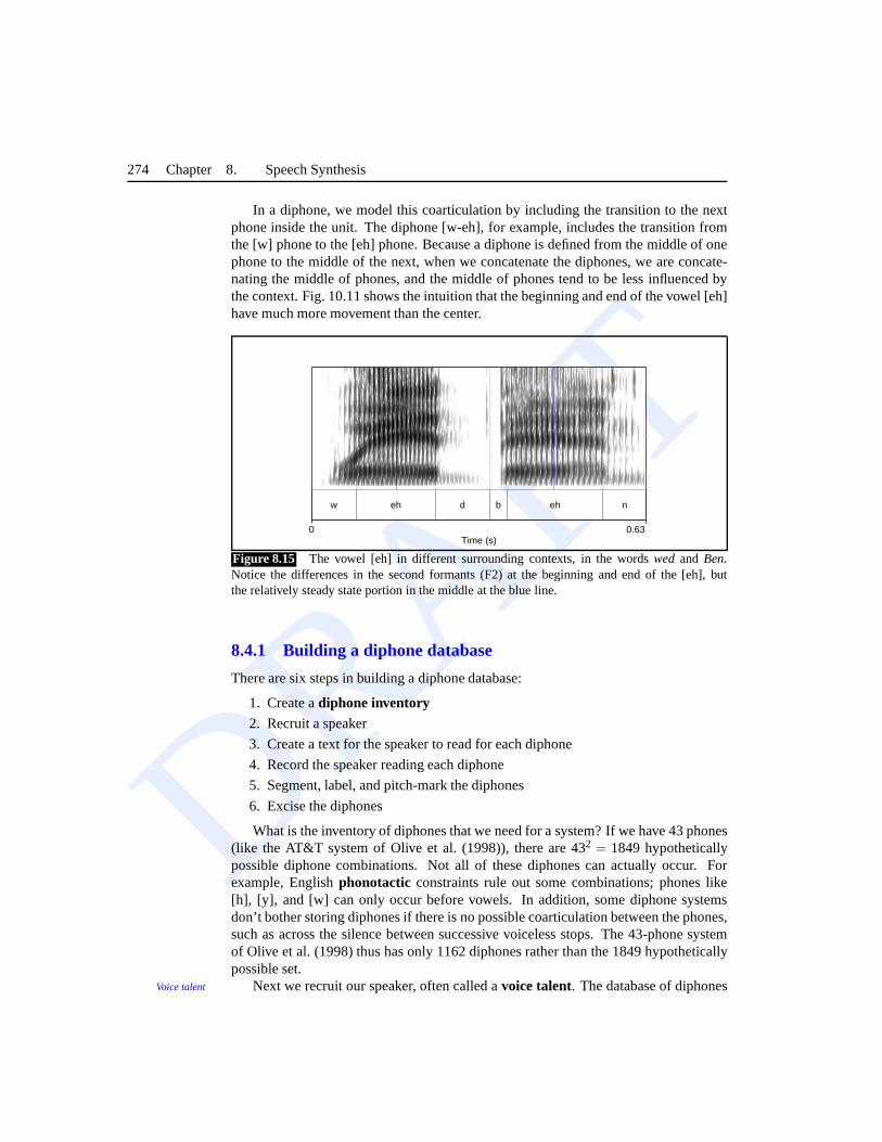
In a diphone, we model this coarticulation by including the transition to the nextphone inside the unit. The diphone [w-eh], for example, includes the transition fromthe [w] phone to the [eh] phone. Because a diphone is defined from the middle of onephone to the middle of the next, when we concatenate the diphones, we are concate-nating the middle of phones, and the middle of phones tend to be less influenced bythe context. Fig. 10.11 shows the intuition that the beginning and end of the vowel [eh]have much more movement than the center.
w eh d b eh n
Time (s)0 0.63
Figure 8.15 The vowel [eh] in different surrounding contexts, in the words wed and Ben.Notice the differences in the second formants (F2) at the beginning and end of the [eh], butthe relatively steady state portion in the middle at the blueline.
8.4.1 Building a diphone database
There are six steps in building a diphone database:
1. Create adiphone inventory2. Recruit a speaker
3. Create a text for the speaker to read for each diphone
4. Record the speaker reading each diphone
5. Segment, label, and pitch-mark the diphones
6. Excise the diphones
What is the inventory of diphones that we need for a system? Ifwe have 43 phones(like the AT&T system of Olive et al. (1998)), there are 432 = 1849 hypotheticallypossible diphone combinations. Not all of these diphones can actually occur. Forexample, Englishphonotactic constraints rule out some combinations; phones like[h], [y], and [w] can only occur before vowels. In addition, some diphone systemsdon’t bother storing diphones if there is no possible coarticulation between the phones,such as across the silence between successive voiceless stops. The 43-phone systemof Olive et al. (1998) thus has only 1162 diphones rather thanthe 1849 hypotheticallypossible set.
Next we recruit our speaker, often called avoice talent. The database of diphonesVoice talent
DRAFT
Section 8.4. Diphone Waveform synthesis 275
for this speaker is called avoice; commercial systems often have multiple voices, suchVoice
as one male and one female voice.We’ll now create a text for the voice talent to say, and recordeach diphone. The
most important thing in recording diphones is to keep them asconsistent as possible;if possible, they should have constant pitch, energy, and duration, so they are easy topaste together without noticeable breaks. We do this by enclosing each diphone to berecorded in acarrier phrase. By putting the diphone in the middle of other phones,Carrier phrase
we keep utterance-final lengthening or initial phone effects from making any diphonelouder or quieter than the others. We’ll need different carrier phrases for consonant-vowel, vowel-consonant, phone-silence, and silence-phone sequences. For example, aconsonant vowel sequence like [b aa] or [b ae] could be embedded between the sylla-bles [t aa] and [m aa]:
pause t aa b aa m aa pausepause t aa b ae m aa pausepause t aa b eh m aa pause...
If we have an earlier synthesizer voice lying around, we usually use that voice toread the prompts out loud, and have our voice talent repeat after the prompts. Thisis another way to keep the pronunciation of each diphone consistent. It is also veryimportant to use a high quality microphone and a quiet room or, better, a studio soundbooth.
Once we have recorded the speech, we need to label and segmentthe two phonesthat make up each diphone. This is usually done by running a speech recognizer inforced alignment mode. In forced alignment mode, a speech recognition is told ex-actly what the phone sequence is; its job is just to find the exact phone boundariesin the waveform. Speech recognizers are not completely accurate at finding phoneboundaries, and so usually the automatic phone segmentation is hand-corrected.
We now have the two phones (for example [b aa]) with hand-corrected boundaries.There are two ways we can create the /b-aa/ diphone for the database. One method is touse rules to decide how far into the phone to place the diphoneboundary. For example,for stops, we put place the diphone boundary 30% of the way into the phone. For mostother phones, we place the diphone boundary 50% into the phone.
A more sophisticated way to find diphone boundaries is to store the entire twophones, and wait to excise the diphones until we are know whatphone we are aboutto concatenate with. In this method, known asoptimal coupling, we take the twoOptimal coupling
(complete, uncut) diphones we need to concatenate, and we check every possible cut-ting point for each diphones, choosing the two cutting points that would make the finalframe of the first diphone acoustically most similar to the end frame of the next diphone(Taylor and Isard, 1991; Conkie and Isard, 1996). Acoustical similar can be measuredby usingcepstral similarity , to be defined in Sec. 9.3.
8.4.2 Diphone concatenation and TD-PSOLA for prosody
We are now ready to see the remaining steps for synthesizing an individual utterance.Assume that we have completed text analysis for the utterance, and hence arrived at a
DRAFT
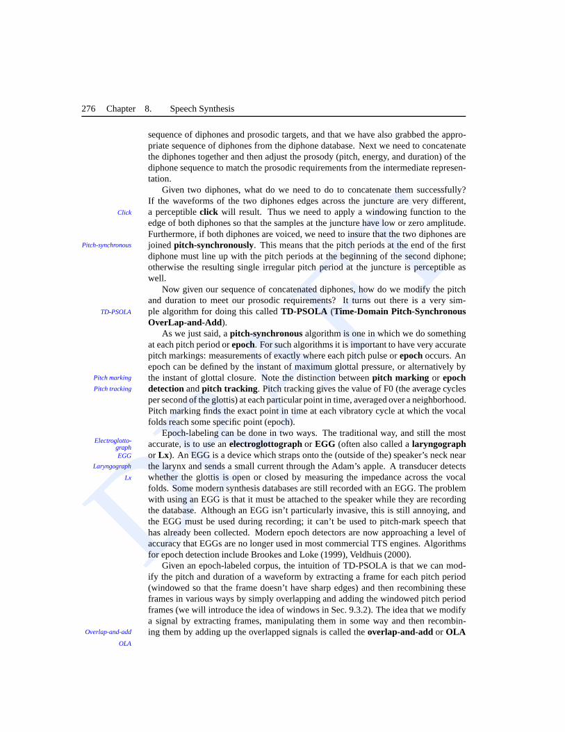
276 Chapter 8. Speech Synthesis
sequence of diphones and prosodic targets, and that we have also grabbed the appro-priate sequence of diphones from the diphone database. Nextwe need to concatenatethe diphones together and then adjust the prosody (pitch, energy, and duration) of thediphone sequence to match the prosodic requirements from the intermediate represen-tation.
Given two diphones, what do we need to do to concatenate them successfully?If the waveforms of the two diphones edges across the juncture are very different,a perceptibleclick will result. Thus we need to apply a windowing function to theClick
edge of both diphones so that the samples at the juncture havelow or zero amplitude.Furthermore, if both diphones are voiced, we need to insure that the two diphones arejoinedpitch-synchronously. This means that the pitch periods at the end of the firstPitch-synchronous
diphone must line up with the pitch periods at the beginning of the second diphone;otherwise the resulting single irregular pitch period at the juncture is perceptible aswell.
Now given our sequence of concatenated diphones, how do we modify the pitchand duration to meet our prosodic requirements? It turns outthere is a very sim-ple algorithm for doing this calledTD-PSOLA (Time-Domain Pitch-SynchronousTD-PSOLA
OverLap-and-Add).As we just said, apitch-synchronousalgorithm is one in which we do something
at each pitch period orepoch. For such algorithms it is important to have very accuratepitch markings: measurements of exactly where each pitch pulse orepochoccurs. Anepoch can be defined by the instant of maximum glottal pressure, or alternatively bythe instant of glottal closure. Note the distinction between pitch marking or epochPitch marking
detectionandpitch tracking . Pitch tracking gives the value of F0 (the average cyclesPitch tracking
per second of the glottis) at each particular point in time, averaged over a neighborhood.Pitch marking finds the exact point in time at each vibratory cycle at which the vocalfolds reach some specific point (epoch).
Epoch-labeling can be done in two ways. The traditional way,and still the mostaccurate, is to use anelectroglottographor EGG (often also called alaryngographElectroglotto-
graphEGG
Laryngograph
or Lx ). An EGG is a device which straps onto the (outside of the) speaker’s neck near
Lx
the larynx and sends a small current through the Adam’s apple. A transducer detectswhether the glottis is open or closed by measuring the impedance across the vocalfolds. Some modern synthesis databases are still recorded with an EGG. The problemwith using an EGG is that it must be attached to the speaker while they are recordingthe database. Although an EGG isn’t particularly invasive,this is still annoying, andthe EGG must be used during recording; it can’t be used to pitch-mark speech thathas already been collected. Modern epoch detectors are now approaching a level ofaccuracy that EGGs are no longer used in most commercial TTS engines. Algorithmsfor epoch detection include Brookes and Loke (1999), Veldhuis (2000).
Given an epoch-labeled corpus, the intuition of TD-PSOLA isthat we can mod-ify the pitch and duration of a waveform by extracting a framefor each pitch period(windowed so that the frame doesn’t have sharp edges) and then recombining theseframes in various ways by simply overlapping and adding the windowed pitch periodframes (we will introduce the idea of windows in Sec. 9.3.2).The idea that we modifya signal by extracting frames, manipulating them in some wayand then recombin-ing them by adding up the overlapped signals is called theoverlap-and-addor OLAOverlap-and-add
OLA
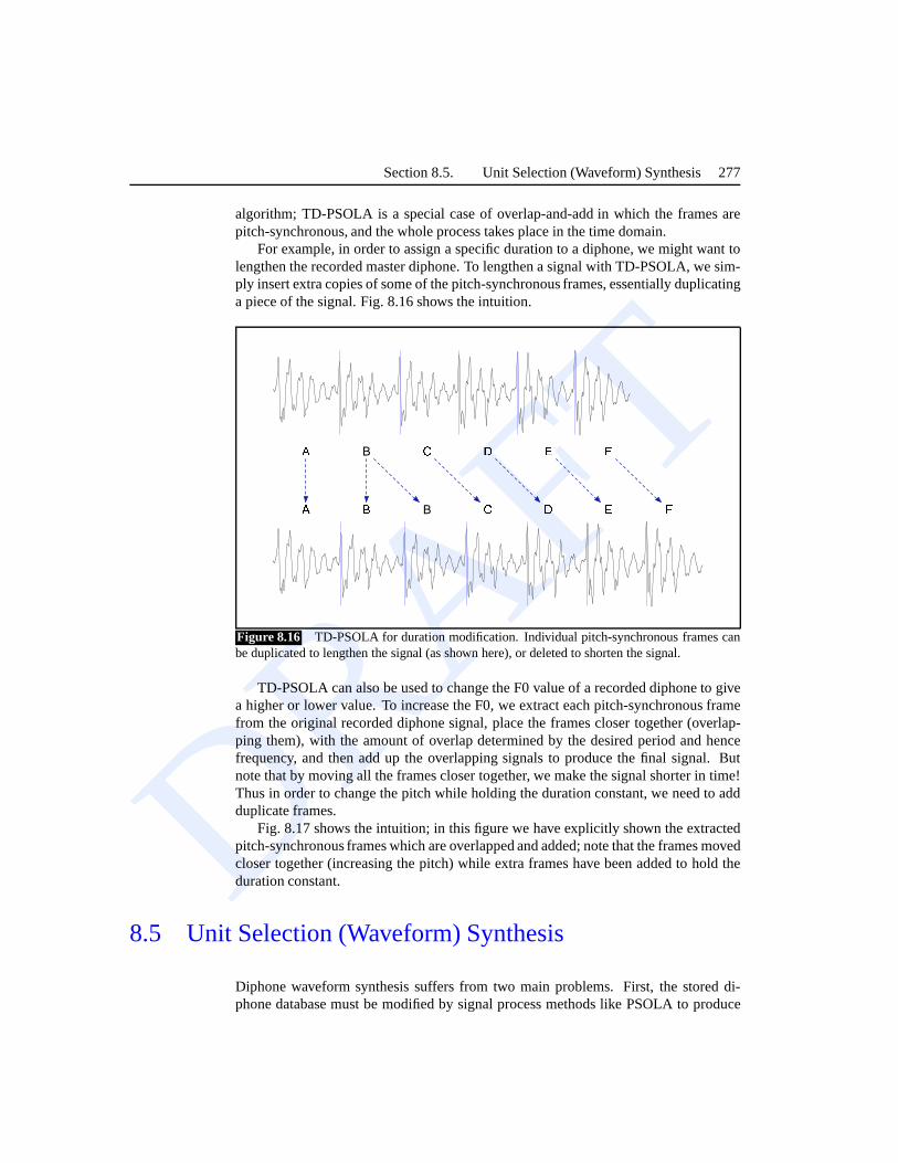
DRAFT
Section 8.5. Unit Selection (Waveform) Synthesis 277
algorithm; TD-PSOLA is a special case of overlap-and-add inwhich the frames arepitch-synchronous, and the whole process takes place in thetime domain.
For example, in order to assign a specific duration to a diphone, we might want tolengthen the recorded master diphone. To lengthen a signal with TD-PSOLA, we sim-ply insert extra copies of some of the pitch-synchronous frames, essentially duplicatinga piece of the signal. Fig. 8.16 shows the intuition.
8 9B : ; <8 9B : ; <=Figure 8.16 TD-PSOLA for duration modification. Individual pitch-synchronous frames canbe duplicated to lengthen the signal (as shown here), or deleted to shorten the signal.
TD-PSOLA can also be used to change the F0 value of a recorded diphone to givea higher or lower value. To increase the F0, we extract each pitch-synchronous framefrom the original recorded diphone signal, place the framescloser together (overlap-ping them), with the amount of overlap determined by the desired period and hencefrequency, and then add up the overlapping signals to produce the final signal. Butnote that by moving all the frames closer together, we make the signal shorter in time!Thus in order to change the pitch while holding the duration constant, we need to addduplicate frames.
Fig. 8.17 shows the intuition; in this figure we have explicitly shown the extractedpitch-synchronous frames which are overlapped and added; note that the frames movedcloser together (increasing the pitch) while extra frames have been added to hold theduration constant.
8.5 Unit Selection (Waveform) Synthesis
Diphone waveform synthesis suffers from two main problems.First, the stored di-phone database must be modified by signal process methods like PSOLA to produce
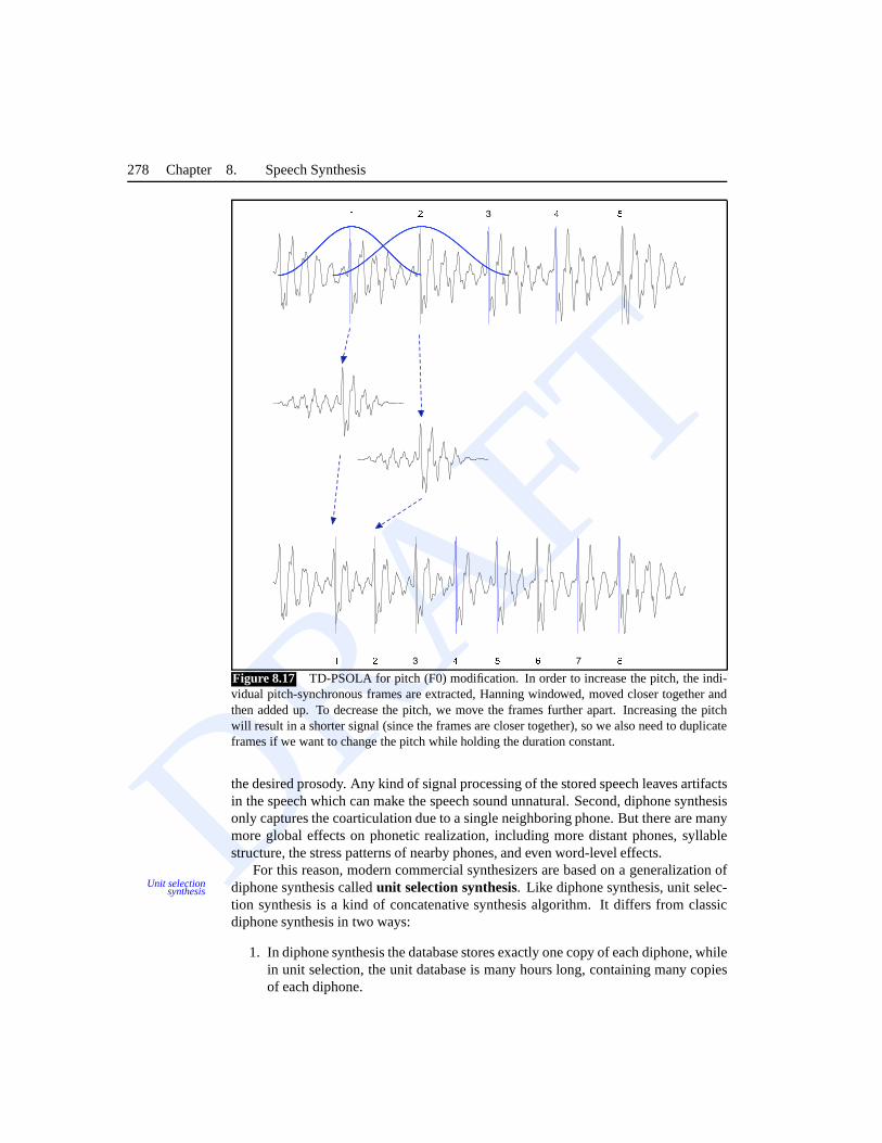
DRAFT
278 Chapter 8. Speech Synthesis
> ? 3 @ A B 7 C
> ? 3 @ A
Figure 8.17 TD-PSOLA for pitch (F0) modification. In order to increase the pitch, the indi-vidual pitch-synchronous frames are extracted, Hanning windowed, moved closer together andthen added up. To decrease the pitch, we move the frames further apart. Increasing the pitchwill result in a shorter signal (since the frames are closer together), so we also need to duplicateframes if we want to change the pitch while holding the duration constant.
the desired prosody. Any kind of signal processing of the stored speech leaves artifactsin the speech which can make the speech sound unnatural. Second, diphone synthesisonly captures the coarticulation due to a single neighboring phone. But there are manymore global effects on phonetic realization, including more distant phones, syllablestructure, the stress patterns of nearby phones, and even word-level effects.
For this reason, modern commercial synthesizers are based on a generalization ofdiphone synthesis calledunit selection synthesis. Like diphone synthesis, unit selec-Unit selection
synthesis
tion synthesis is a kind of concatenative synthesis algorithm. It differs from classicdiphone synthesis in two ways:
1. In diphone synthesis the database stores exactly one copyof each diphone, whilein unit selection, the unit database is many hours long, containing many copiesof each diphone.
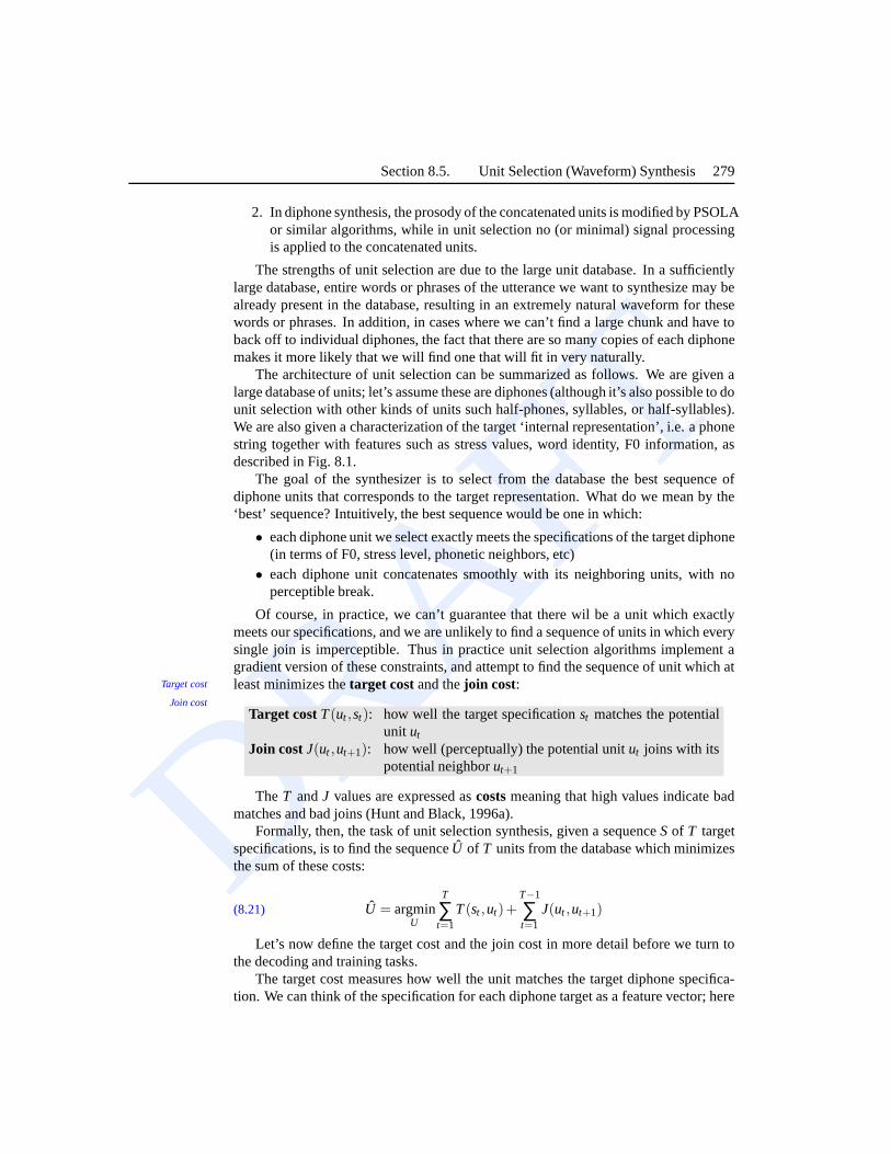
DRAFT
Section 8.5. Unit Selection (Waveform) Synthesis 279
2. In diphone synthesis, the prosody of the concatenated units is modified by PSOLAor similar algorithms, while in unit selection no (or minimal) signal processingis applied to the concatenated units.
The strengths of unit selection are due to the large unit database. In a sufficientlylarge database, entire words or phrases of the utterance we want to synthesize may bealready present in the database, resulting in an extremely natural waveform for thesewords or phrases. In addition, in cases where we can’t find a large chunk and have toback off to individual diphones, the fact that there are so many copies of each diphonemakes it more likely that we will find one that will fit in very naturally.
The architecture of unit selection can be summarized as follows. We are given alarge database of units; let’s assume these are diphones (although it’s also possible to dounit selection with other kinds of units such half-phones, syllables, or half-syllables).We are also given a characterization of the target ‘internalrepresentation’, i.e. a phonestring together with features such as stress values, word identity, F0 information, asdescribed in Fig. 8.1.
The goal of the synthesizer is to select from the database thebest sequence ofdiphone units that corresponds to the target representation. What do we mean by the‘best’ sequence? Intuitively, the best sequence would be one in which:
• each diphone unit we select exactly meets the specificationsof the target diphone(in terms of F0, stress level, phonetic neighbors, etc)• each diphone unit concatenates smoothly with its neighboring units, with no
perceptible break.
Of course, in practice, we can’t guarantee that there wil be aunit which exactlymeets our specifications, and we are unlikely to find a sequence of units in which everysingle join is imperceptible. Thus in practice unit selection algorithms implement agradient version of these constraints, and attempt to find the sequence of unit which atleast minimizes thetarget costand thejoin cost:Target cost
Join costTarget costT(ut ,st): how well the target specificationst matches the potential
unit ut
Join costJ(ut ,ut+1): how well (perceptually) the potential unitut joins with itspotential neighborut+1
TheT andJ values are expressed ascostsmeaning that high values indicate badmatches and bad joins (Hunt and Black, 1996a).
Formally, then, the task of unit selection synthesis, givena sequenceSof T targetspecifications, is to find the sequenceU of T units from the database which minimizesthe sum of these costs:
U = argminU
T
∑t=1
T(st ,ut)+T−1
∑t=1
J(ut ,ut+1)(8.21)
Let’s now define the target cost and the join cost in more detail before we turn tothe decoding and training tasks.
The target cost measures how well the unit matches the targetdiphone specifica-tion. We can think of the specification for each diphone target as a feature vector; here
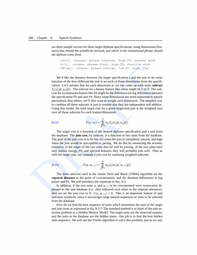
DRAFT
280 Chapter 8. Speech Synthesis
are three sample vectors for three target diphone specifications, using dimensions (fea-tures) likeshould the syllable be stressed, andwhere in the intonational phrase shouldthe diphone come from:
/ih-t/, +stress, phrase internal, high F0, content word
/n-t/, -stress, phrase final, high F0, function word
/dh-ax/, -stress, phrase initial, low F0, word ‘the’
We’d like the distance between the target specifications and the unit to be somefunction of the how different the unit is on each of these dimensions from the specifi-cation. Let’s assume that for each dimensionp, we can come up with somesubcostTp(st [p],u j [p]). The subcost for a binary feature likestressmight be 1 or 0. The sub-cost for a continuous feature like F0 might be the difference(or log difference) betweenthe specification F0 and unit F0. Since some dimensions are more important to speechperceptions than others, we’ll also want to weight each dimension. The simplest wayto combine all these subcosts is just to assume that they are independent and additive.Using this model, the total target cost for a given target/unit pair is the weighted sumover all these subcosts for each feature/dimension:
T(st ,u j) =P
∑p=1
wpTp(st [p],u j [p])(8.22)
The target cost is a function of the desired diphone specification and a unit fromthe database. Thejoin cost, by contrast, is a function of two units from the database.The goal of the join cost is to be low (0) when the join is completely natural, and highwhen the join would be perceptible or jarring. We do this by measuring the acousticsimilarity of the edges of the two units that we will be joining. If the two units havevery similar energy, F0, and spectral features, they will probably join well. Thus aswith the target cost, we compute a join cost by summing weighted subcosts:
J(ut ,ut+1) =P
∑p=1
wpJp(ut [p],ut+1[p])(8.23)
The three subcosts used in the classic Hunt and Black (1996b)algorithm are thecepstral distanceat the point of concatenation, and the absolute differencesin logpower and F0. We will introduce the cepstrum in Sec. 9.3.
In addition, if the two unitsut andut+1 to be concatenated were consecutive di-phones in the unit database (i.e. they followed each other inthe original utterance),then we set the join cost to 0:J(ut ,ut+1) = 0. This is an important feature of unitselection synthesis, since it encourages large natural sequences of units to be selectedfrom the database.
How do we find the best sequence of units which minimizes the sum of the targetand join costs as expressed in Eq. 8.21? The standard method is to think of the unit se-lection problem as a Hidden Markov Model. The target units are the observed outputs,and the units in the database are the hidden states. Our job isto find the best hiddenstate sequence. We will use the Viterbi algorithm to solve this problem, just as we saw
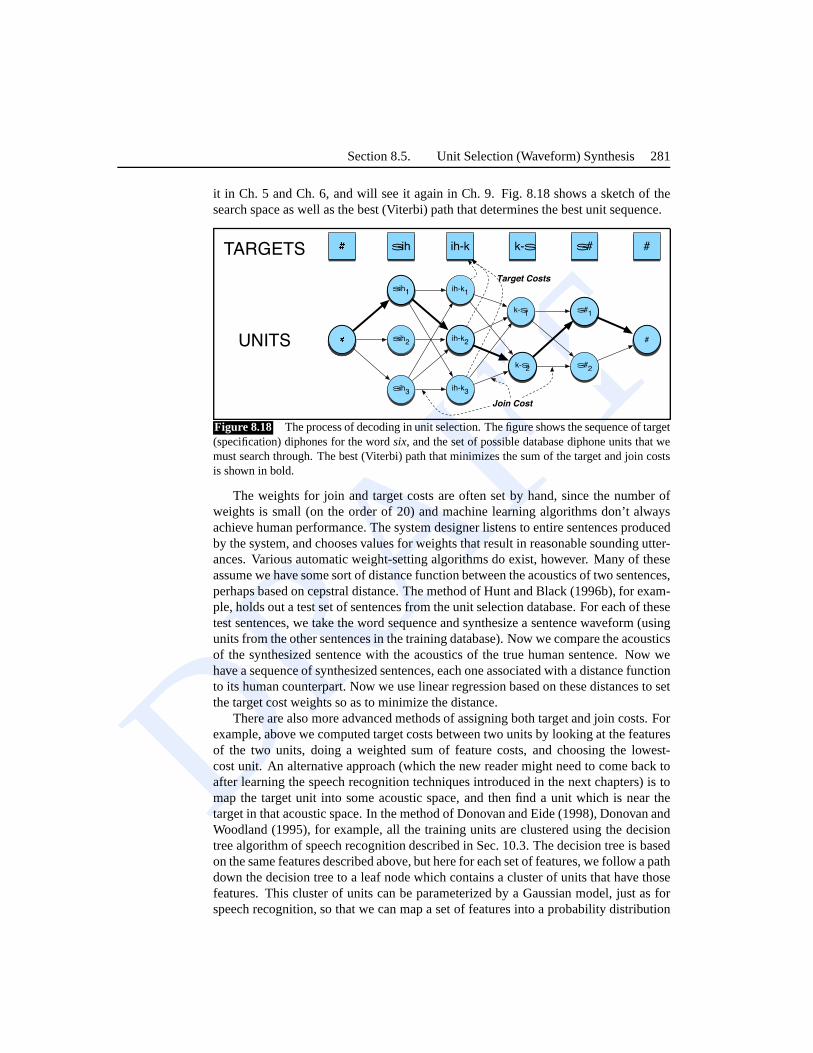
DRAFT
Section 8.5. Unit Selection (Waveform) Synthesis 281
it in Ch. 5 and Ch. 6, and will see it again in Ch. 9. Fig. 8.18 shows a sketch of thesearch space as well as the best (Viterbi) path that determines the best unit sequence.
D s-ih1
Es-ih ih-k k-s s-# #
s-ih2
s-ih3
ih-k1
ih-k2
ih-k3
k-s1
k-s2
s-#1
s-#2
#
TARGETS
UNITS
Join Cost
Target Costs
Figure 8.18 The process of decoding in unit selection. The figure shows the sequence of target(specification) diphones for the wordsix, and the set of possible database diphone units that wemust search through. The best (Viterbi) path that minimizesthe sum of the target and join costsis shown in bold.
The weights for join and target costs are often set by hand, since the number ofweights is small (on the order of 20) and machine learning algorithms don’t alwaysachieve human performance. The system designer listens to entire sentences producedby the system, and chooses values for weights that result in reasonable sounding utter-ances. Various automatic weight-setting algorithms do exist, however. Many of theseassume we have some sort of distance function between the acoustics of two sentences,perhaps based on cepstral distance. The method of Hunt and Black (1996b), for exam-ple, holds out a test set of sentences from the unit selectiondatabase. For each of thesetest sentences, we take the word sequence and synthesize a sentence waveform (usingunits from the other sentences in the training database). Now we compare the acousticsof the synthesized sentence with the acoustics of the true human sentence. Now wehave a sequence of synthesized sentences, each one associated with a distance functionto its human counterpart. Now we use linear regression basedon these distances to setthe target cost weights so as to minimize the distance.
There are also more advanced methods of assigning both target and join costs. Forexample, above we computed target costs between two units bylooking at the featuresof the two units, doing a weighted sum of feature costs, and choosing the lowest-cost unit. An alternative approach (which the new reader might need to come back toafter learning the speech recognition techniques introduced in the next chapters) is tomap the target unit into some acoustic space, and then find a unit which is near thetarget in that acoustic space. In the method of Donovan and Eide (1998), Donovan andWoodland (1995), for example, all the training units are clustered using the decisiontree algorithm of speech recognition described in Sec. 10.3. The decision tree is basedon the same features described above, but here for each set offeatures, we follow a pathdown the decision tree to a leaf node which contains a clusterof units that have thosefeatures. This cluster of units can be parameterized by a Gaussian model, just as forspeech recognition, so that we can map a set of features into aprobability distribution
DRAFT
282 Chapter 8. Speech Synthesis
over cepstral values, and hence easily compute a distance between the target and aunit in the database. As for join costs, more sophisticated metrics make use of howperceivable a particular join might be (Wouters and Macon, 1998; Syrdal and Conkie,2004; Bulyko and Ostendorf, 2001).
8.6 Evaluation
Speech synthesis systems are evaluated by human listeners.The development of agood automatic metric for synthesis evaluation, that wouldeliminate the need for ex-pensive and time-consuming human listening experiments, remains an open and exitingresearch topic.
The minimal evaluation metric for speech synthesis systemsis intelligibility : theIntelligibility
ability of a human listener to correctly interpret the wordsand meaning of the synthe-sized utterance. A further metric isquality ; an abstract measure of the naturalness,Quality
fluency, or clarity of the speech.The most local measures of intelligibility test the abilityof a listener to discriminate
between two phones. TheDiagnostic Rhyme Test(DRT) (Voiers et al., 1975) testsDiagnostic RhymeTest
DRT the intelligibility of initial consonants. It is based on 96pairs of confusable rhymingwords which differ only in a single phonetic feature, such as(dense/tense) orbond/pond(differing in voicing) ormean/beator neck/deck(differing in nasality), and so on. Foreach pair, listeners hear one member of the pair, and indicate which they think it is.The percentage of right answers is then used as an intelligibility metric. TheModifiedRhyme Test (MRT ) (House et al., 1965) is a similar test based on a different set ofModified Rhyme
TestMRT 300 words, consisting of 50 sets of 6 words. Each 6-word set differs in either initial
or final consonants (e.g.,went, sent, bent, dent, tent, rent or bat, bad, back, bass, ban,bath). Listeners are again given a single word and must identify from a closed list ofsix words; the percentage of correct identifications is again used as an intelligibilitymetric.
Since context effects are very important, both DRT and MRT words are embeddedin carrier phrases like the following:Carrier phrase
Now we will say <word> again.
In order to test larger units than single phones, we can usesemantically unpre-dictable sentences(SUS) (Benoıt et al., 1996). These are sentences constructed bySUS
taking a simple POS template likeDET ADJ NOUN VERB DET NOUN and insertingrandom English words in the slots, to produce sentences like
The unsure steaks closed the fish.
Measures of intelligibility like DRT/MRT and SUS are designed to factor out therole of context in measuring intelligibility. While this allows us to get a carefullycontrolled measure of a system’s intelligibility, such acontextual or semantically un-predictable sentences aren’t a good fit to how TTS is used in most commercial appli-cations. Thus in commercial applications instead of DRT or SUS, we generally testintelligibility using situations that mimic the desired applications; reading addressesout loud, reading lines of news text, and so on.
DRAFTSection 8.6. Evaluation 283
To further evaluate thequality of the synthesized utterances, we can play a sentencefor a listener and ask them to give amean opinion score(MOS), a rating of how goodMOS
the synthesized utterances are, usually on a scale from 1-5.We can then comparesystems by comparing their MOS scores on the same sentences (using, e.g., t-tests totest for significant differences).
If we are comparing exactly two systems (perhaps to see if a particular changeactually improved the system), we can useAB tests In AB tests, we play the sameAB tests
sentence synthesized by two different systems (an A and a B system). The humanlistener chooses which of the two utterances they like better. We can do this for 50sentences and compare the number of sentences preferred foreach systems. In orderto avoid ordering preferences, for each sentence we must present the two synthesizedwaveforms in random order.
Bibliographical and Historical NotesAs we noted at the beginning of the chapter, speech synthesisis one of the earliest fieldsof speech and language processing. The 18th century saw a number of physical modelsof the articulation process, including the von Kempelen model mentioned above, aswell as the 1773 vowel model of Kratzenstein in Copenhagen using organ pipes.
But the modern era of speech synthesis can clearly be said to have arrived by theearly 1950’s, when all three of the major paradigms of waveform synthesis had beenproposed (formant synthesis, articulatory synthesis, andconcatenative synthesis).
Concatenative synthesis seems to have been first proposed byHarris (1953) at BellLaboratories, who literally spliced together pieces of magnetic tape corresponding tophones. Harris’s proposal was actually more like unit selection synthesis than diphonesynthesis, in that he proposed storing multiple copies of each phone, and proposedthe use of a join cost (choosing the unit with the smoothest formant transitions withthe neighboring unit). Harris’s model was based on the phone, rather than diphone,resulting in problems due to coarticulation. Peterson et al. (1958) added many of thebasic ideas of unit selection synthesis, including the use of diphones, a database withmultiple copies of each diphone with differing prosody, andeach unit labeled with in-tonational features including F0, stress, and duration, and the use of join costs basedon F0 and formant distant between neighboring units. They also proposed microcon-catenation techniques like windowing the waveforms. The Peterson et al. (1958) modelwas purely theoretical, however, and concatenative synthesis was not implemented un-til the 1960’s and 1970’s, when diphone synthesis was first implemented (Dixon andMaxey, 1968; Olive, 1977). Later diphone systems included larger units such as con-sonant clusters (Olive and Liberman, 1979). Modern unit selection, including the ideaof large units of non-uniform length, and the use of a target cost, was invented by Sag-isaka (1988), Sagisaka et al. (1992). Hunt and Black (1996b)formalized the model,and put it in the form in which we have presented it in this chapter in the context of theATR CHATR system (Black and Taylor, 1994). The idea of automatically generatingsynthesis units by clustering was first invented by Nakajimaand Hamada (1988), but
DRAFT
284 Chapter 8. Speech Synthesis
was developed mainly by (Donovan, 1996) by incorporating decision tree clustering al-gorithms from speech recognition. Many unit selection innovations took place as partof the ATT NextGen synthesizer (Syrdal et al., 2000; Syrdal and Conkie, 2004).
We have focused in this chapter on concatenative synthesis,but there are two otherparadigms for synthesis:formant synthesis, in which we attempt to build rules whichgenerate artificial spectra, including especially formants, andarticulatory synthesis,in which we attempt to directly model the physics of the vocaltract and articulatoryprocess.
Formant synthesizersoriginally were inspired by attempts to mimic human speechby generating artificial spectrograms. The Haskins Laboratories Pattern Playback Ma-chine generated a sound wave by painting spectrogram patterns on a moving trans-parent belt, and using reflectance to filter the harmonics of awaveform (Cooper et al.,1951); other very early formant synthesizers include Lawrence (1953) and Fant (3951).Perhaps the most well-known of the formant synthesizers were theKlatt formant syn-thesizerand its successor systems, including the MITalk system (Allen et al., 1987),and the Klattalk software used in Digital Equipment Corporation’s DECtalk (Klatt,1982). See Klatt (1975) for details.
Articulatory synthesizers attempt to synthesize speech by modeling the physicsof the vocal tract as an open tube. Representative models, both early and somewhatmore recent include Stevens et al. (1953), Flanagan et al. (1975), Fant (1986) See Klatt(1975) and Flanagan (1972) for more details.
Development of the text analysis components of TTS came somewhat later, as tech-niques were borrowed from other areas of natural language processing. The input toearly synthesis systems was not text, but rather phonemes (typed in on punched cards).The first text-to-speech system to take text as input seems tohave been the system ofUmeda and Teranishi (Umeda et al., 1968; Teranishi and Umeda, 1968; Umeda, 1976).The system included a lexicalized parser which was used to assign prosodic bound-aries, as well as accent and stress; the extensions in Coker et al. (1973) added addi-tional rules, for example for deaccenting light verbs and explored articulatory modelsas well. These early TTS systems used a pronunciation dictionary for word pronuncia-tions. In order to expand to larger vocabularies, early formant-based TTS systems suchas MITlak (Allen et al., 1987) used letter-to-sound rules instead of a dictionary, sincecomputer memory was far too expensive to store large dictionaries.
Modern grapheme-to-phoneme models derive from the influential early probabilis-tic grapheme-to-phoneme model of Lucassen and Mercer (1984), which was originallyproposed in the context of speech recognition. The widespread use of such machinelearning models was delayed, however, because early anecdotal evidence suggestedthat hand-written rules worked better than e.g., the neuralnetworks of Sejnowski andRosenberg (1987). The careful comparisons of Damper et al. (1999) showed that ma-chine learning methods were in generally superior. A numberof such models make useof pronunciation by analogy (Byrd and Chodorow, 1985; ?; Daelemans and van denBosch, 1997; Marchand and Damper, 2000) or latent analogy (Bellegarda, 2005);HMMs (Taylor, 2005) have also been proposed. The most recentwork makes useof joint graphonemodels, in which the hidden variables are phoneme-graphemepairsGraphone
and the probabilistic model is based on joint rather than conditional likelihood (Deligneet al., 1995; Luk and Damper, 1996; Galescu and Allen, 2001; Bisani and Ney, 2002;
DRAFTSection 8.6. Evaluation 285
Chen, 2003).There is a vast literature on prosody. Besides the ToBI and TILT models described
above, other important computational models include theFujisaki model (FujisakiFujisaki
and Ohno, 1997). IViE (Grabe, 2001) is an extension of ToBI that focuses on labellingdifferent varieties of English (Grabe et al., 2000). There is also much debate on theunits of intonational structure (intonational phrases (Beckman and Pierrehumbert,1986),intonation units (Du Bois et al., 1983) ortone units (Crystal, 1969)), and theirIntonation unit
Tone unit relation to clauses and other syntactic units (Chomsky and Halle, 1968; Langendoen,1975; Streeter, 1978; Hirschberg and Pierrehumbert, 1986;Selkirk, 1986; Nespor andVogel, 1986; Croft, 1995; Ladd, 1996; Ford and Thompson, 1996; Ford et al., 1996).
One of the most exciting new paradigms for speech synthesis is HMM synthesis,HMM synthesis
first proposed by Tokuda et al. (1995b) and elaborated in Tokuda et al. (1995a), Tokudaet al. (2000), and Tokuda et al. (2003). See also the textbooksummary of HMM syn-thesis in Taylor (2008).
More details on TTS evaluation can be found in Huang et al. (2001) and Gibbonet al. (2000). Other descriptions of evaluation can be foundin the annual speech syn-thesis competition called theBlizzard Challenge (Black and Tokuda, 2005; Bennett,Blizzard
Challenge
2005).Much recent work on speech synthesis has focused on generating emotional speech
(Cahn, 1990; Bulut1 et al., 2002; Hamza et al., 2004; Eide et al., 2004; Lee et al., 2006;Schroder, 2006, inter alia)
Two classic text-to-speech synthesis systems are described in Allen et al. (1987)(the MITalk system) and Sproat (1998b) (the Bell Labs system). Recent textbooksinclude Dutoit (1997), Huang et al. (2001), Taylor (2008), and Alan Black’s online lec-ture notes athttp://festvox.org/festtut/notes/festtut_toc.html .Influential collections of papers include van Santen et al. (1997), Sagisaka et al. (1997),Narayanan and Alwan (2004). Conference publications appear in the main speech engi-neering conferences (INTERSPEECH,IEEE ICASSP), and theSpeech Synthesis Work-shops. Journals includeSpeech Communication, Computer Speech and Language, theIEEE Transactions on Audio, Speech, and Language Processing, and theACM Trans-actions on Speech and Language Processing.
Exercises8.1 Implement the text normalization routine that deals withMONEY, i.e. mapping
strings of dollar amounts like$45, $320, and$4100to words (either writing codedirectly or designing an FST). If there are multiple ways to pronounce a numberyou may pick your favorite way.
8.2 Implement the text normalization routine that deals withNTEL, i.e. seven-digitphone numbers like555-1212, 555-1300, and so on. You should use a combina-
DRAFT
286 Chapter 8. Speech Synthesis
tion of thepaired andtrailing unit methods of pronunciation for the last fourdigits. (Again you may either write code or design an FST).
8.3 Implement the text normalization routine that deals with typeDATE in Fig. 8.1.2
8.4 Implement the text normalization routine that deals with typeNTIME in Fig. 8.1.2.
8.5 (Suggested by Alan Black). Download the free Festival speech synthesizer. Aug-ment the lexicon to correctly pronounce the names of everyone in your class.
8.6 Download the Festival synthesizer. Record and train a diphone synthesizer usingyour own voice.


![“YEAH RIGHT”web2.cs.columbia.edu/~julia/courses/CS6998/Student... · intent to deceive on the speaker’s part [4]. Like a Grounding Act, sarcastic speech requires collaboration](https://static.fdocuments.us/doc/165x107/5f62bc2948961021bd3a7727/aoeyeah-rightaweb2cs-juliacoursescs6998student-intent-to-deceive-on.jpg)