Chapter 8 Sorting 1CSCI 3333 Data Structures. Outline Basic definitions Sorting algorithms –...
24
Chapter 8 Sorting 1 CSCI 3333 Data Structures
-
Upload
dillon-greenland -
Category
Documents
-
view
241 -
download
9
Transcript of Chapter 8 Sorting 1CSCI 3333 Data Structures. Outline Basic definitions Sorting algorithms –...

CSCI 3333 Data Structures 1
Chapter 8
Sorting

CSCI 3333 Data Structures 2
Outline
• Basic definitions• Sorting algorithms
– Bubble sort– Insertion sort– Selection sort– Quick sort– Shell sort– Merge sort
• Example programs
CSCI 3333 Data Structures 3
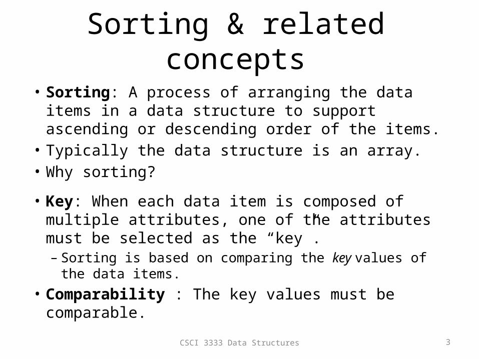
Sorting & related concepts
• Sorting: A process of arranging the data items in a data structure to support ascending or descending order of the items.
• Typically the data structure is an array.• Why sorting?
• Key: When each data item is composed of multiple attributes, one of the attributes must be selected as the “key”.– Sorting is based on comparing the key values of the data
items.• Comparability : The key values must be comparable.

CSCI 3333 Data Structures 4
Sorting & related concepts
• There exist various sorting algorithms– Bubble sort– Insertion sort– Selection sort– Quick sort– Shell sort– Merge sort– …

CSCI 3333 Data Structures 5
Bubble sort
• Source: http://www.leepoint.net/notes-java/data/arrays/32arraybubblesort.html
• A simple sorting algorithm of O(N2).• Also called ‘sink sort’. Why?• Exercise: Sort an array of the five items with bubble sort and count the
number of comparisons.• Question: How does the ‘sorted section’ grow with each pass?

CSCI 3333 Data Structures 6
Selection sort
• Source: http://www.leepoint.net/notes-java/data/arrays/31arrayselectionsort.html
• O(N2)• Exercise: Sort an array of the five items with selection sort and count the number
of comparisons.• Question: How does the ‘sorted section’ grow with each pass? Where is the
‘sorted section’ located?

CSCI 3333 Data Structures 7
Insertion sort
• O(N2)• Only appropriate for small N.• A good algorithm when most items are already sorted.• More efficient in practice than most other simple quadratic algorithms such
as selection sort or bubble sort; the best case (nearly sorted input) is O(n).

CSCI 3333 Data Structures 8
Insertion sort: example

CSCI 3333 Data Structures 9
Insertion sort: example
CSCI 3333 Data Structures 10
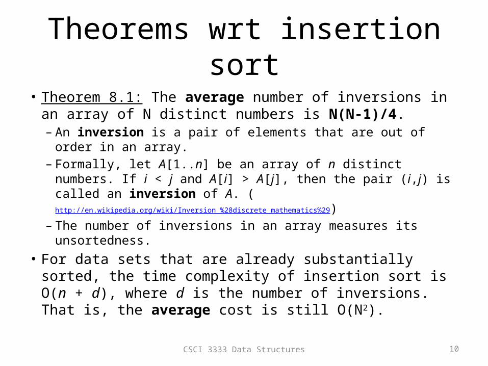
Theorems wrt insertion sort
• Theorem 8.1: The average number of inversions in an array of N distinct numbers is N(N-1)/4.– An inversion is a pair of elements that are out of order in an
array.– Formally, let A[1..n] be an array of n distinct numbers. If i < j and
A[i] > A[j], then the pair (i,j) is called an inversion of A. (http://en.wikipedia.org/wiki/Inversion_%28discrete_mathematics%29)
– The number of inversions in an array measures its unsortedness.• For data sets that are already substantially sorted, the time
complexity of insertion sort is O(n + d), where d is the number of inversions. That is, the average cost is still O(N2).
CSCI 3333 Data Structures 11
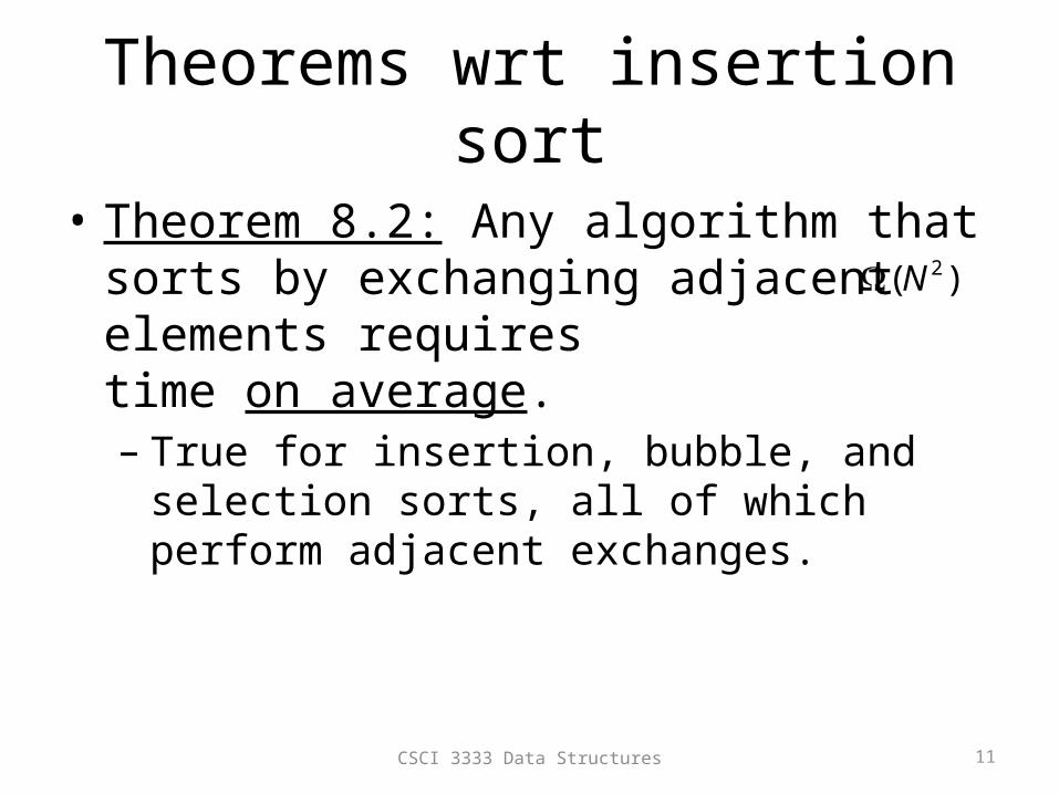
Theorems wrt insertion sort
• Theorem 8.2: Any algorithm that sorts by exchanging adjacent elements requires time on average.– True for insertion, bubble, and selection sorts, all
of which perform adjacent exchanges.
2( )N

CSCI 3333 Data Structures 12
Insertion vs Selection sort
• Source: http://en.wikipedia.org/wiki/Insertion_sort – While insertion sort typically makes fewer comparisons than
selection sort, it requires more writes because the inner loop can require shifting large sections of the sorted portion of the array.
– In general, insertion sort will write to the array O(n2) times, whereas selection sort will write only O(n) times.
Question: Do you agree with the above statement? Is there a way of verifying it?
– For this reason selection sort may be preferable in cases where writing to memory is significantly more expensive than reading, such as with EEPROM or flash memory.
CSCI 3333 Data Structures 13
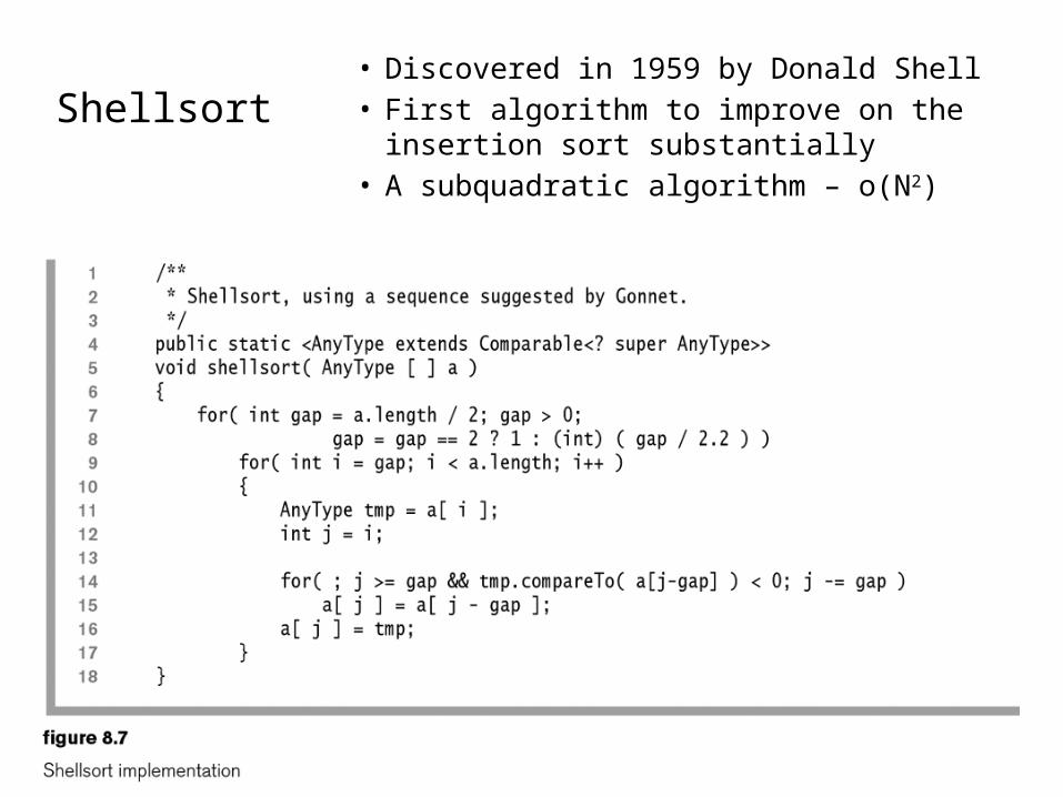
Shellsort• Discovered in 1959 by Donald Shell• First algorithm to improve on the
insertion sort substantially• A subquadratic algorithm – o(N2)

CSCI 3333 Data Structures 14
Shellsort• Shellsort uses a sequence called the increment sequence.
– After a phase, using some increment hk, we have for every i where i + hk is a valid index; all elements spaced hk apart are sorted.
– The array is then said to be hk-sorted.
• Exercise 1: Shellsort the array below using the shellsort() method shown above.
• Exercise 2: Repeat the shellsort but use the sequence {1,3,5}. Compare their performance.
• Exercise 3: Would the sequence {1,3,7} be better?

CSCI 3333 Data Structures 15
Shellsort
• Also called diminishing gap sort– For each gap, it performs a gap insertion sort.– When gap becomes 1, it performs exactly the
insertion sort.• Question: The shell sort contains three loops.
How can it be possible that it’s more efficient than the insertion sort, which contains only two loops?

CSCI 3333 Data Structures 16
Shellsort• The running time of Shellsort depends heavily on the choice of
increment sequences.• Better sequences (than what Shell proposed) are known.
– Odd gaps only: When the gap is even, add 1 to it.– Divide the gap by 2.2, instead of 2 as in the Shell’s increments
CSCI 3333 Data Structures 17
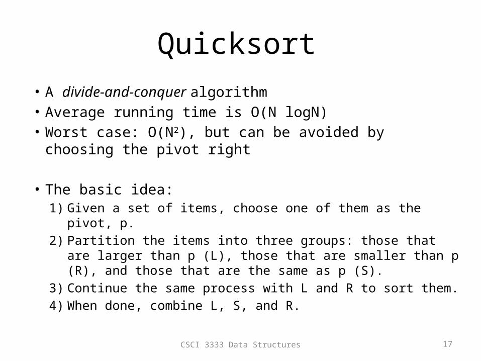
Quicksort
• A divide-and-conquer algorithm• Average running time is O(N logN)• Worst case: O(N2), but can be avoided by choosing the pivot
right
• The basic idea: 1) Given a set of items, choose one of them as the pivot, p.2) Partition the items into three groups: those that are larger than
p (L), those that are smaller than p (R), and those that are the same as p (S).
3) Continue the same process with L and R to sort them.4) When done, combine L, S, and R.

CSCI 3333 Data Structures 18
• Basic process
Quicksort
CSCI 3333 Data Structures 19
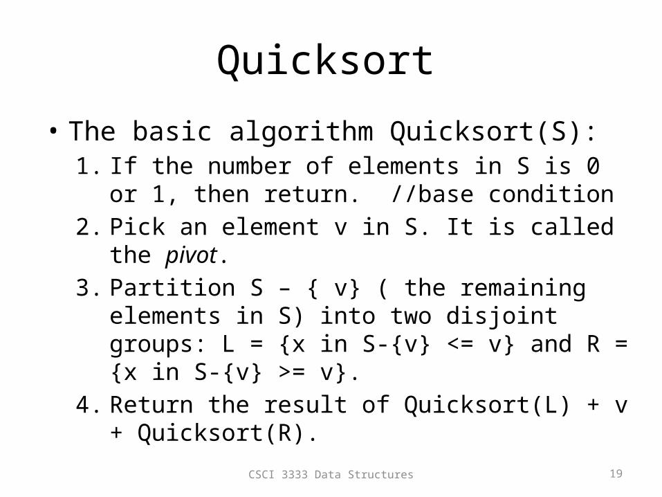
Quicksort
• The basic algorithm Quicksort(S):1. If the number of elements in S is 0 or 1, then
return. //base condition2. Pick an element v in S. It is called the pivot. 3. Partition S – { v} ( the remaining elements in S)
into two disjoint groups: L = {x in S-{v} <= v} and R = {x in S-{v} >= v}.
4. Return the result of Quicksort(L) + v + Quicksort(R).

CSCI 3333 Data Structures 20
Example implementation
• Quicksort (a[ ], low, high)1) If size(a) < CUTOFF then
insertionSort (a,low,high);2) Else
1) Sort the low, middle, high elements2) Choose the middle as the pivot3) Place the pivot at the high-1 position4) Partitioning the range from low to
pivot-1:i. Search from low toward the pivot until an
item >= the pivot is found (let i = the index of that item)
ii. Search from the pivot down toward low until an item <= the pivot is found (let j = the index of that item)
5) Place the pivot to the right position, i.6) Quicksort (a, low, i-1)7) Quicksort (a, i+1, high)

CSCI 3333 Data Structures 21
Quicksort: exampleIndex a [ ]
0 170
1 200
2 150
3 500
4 210
5 220
6 100
Mid = 3
Pivot =
i =
j =

CSCI 3333 Data Structures 22
Quicksort: exampleIndex a [ ]
0 500
1 150
2 220
3 100
4 150
5 200
6 150
Mid = 3
Pivot =
i =
j =
CSCI 3333 Data Structures 23
Analysis of quicksort
• Best case: O(N logN)– In each phase, the pivot partitions the set into two
equally sized subsets (logN)– Each phase incurs linear overhead (N)
• Worst case: O(N2)– When the smallest (or the largest) element is
chosen as the pivot• Average case: O(N logN)

CSCI 3333 Data Structures 24
Exercises
• Ex 8.1: Sort the sequence 8,1,4,1,5,9,2,6,5 usinga) Insertion sortb) Shellsort for the increments {1,3,5}c) Quicksort, with the middle element as the pivot
and no cutoff (show all steps)d) Quicksort, with median-of-three pivot selection
and a cutoff of 3