1 Probabilistic grammars as models of gradience in language processing Matthew W. Crocker

Chapter 8
Probabilistic Language Models
In this chapter, we consider probability models that are specifically linguistic:Hidden Markov Models (HMMs) and Probabilistic Context-free Grammars
(PCFGs).These models can be used to directly encode probability values in linguis-
tic formalism. While such models have well-understood formal properties andare widely used in computational research, they are extremely controversialin the theory of language. It is a hotly debated question whether grammaritself should incorporate probabilistic information.
8.1 The Chain Rule
To understand HMMs, we must first understand the Chain Rule. The ChainRule is one simple consequence of the definition of conditional probability:the joint probability of some set of events a1, a2, a3, a4 can also be expressedas a ‘chain’ of conditional probabilities, e.g.:
(8.1) p(a1, a2, a3, a4) = p(a1)p(a2|a1)p(a3|a1, a2)p(a4|a1, a2, a3)
This follows algebraically from the definition of conditional probability. Ifwe substitute by the definition of conditional probability for each of theconditional probabilities in the preceeding equation and then cancel terms,we get the original joint probability.
142

CHAPTER 8. PROBABILISTIC LANGUAGE MODELS 143
(8.2) p(a1, a2, a3, a4) = p(a1) × p(a2|a1) × p(a3|a1, a2) × p(a4|a1, a2, a3)
= p(a1) ×p(a1,a2)
p(a1)× p(a1,a2,a3)
p(a1,a2)× p(a1,a2,a3,a4)
p(a1,a2,a3)
= p(a1, a2, a3, a4)
Notice also that the chain rule can be used to express any dependency amongthe terms of the original joint probability. For example:
(8.3) p(a1, a2, a3, a4) = p(a4)p(a3|a4)p(a2|a3, a4)p(a1|a2, a3, a4)
Here we express the first events as conditional on the later events, ratherthan vice versa.
8.2 N-gram models
Another preliminary to both HMMs and PCGFs are N-gram models. Theseare the very simplest kind of statistical language model. The basic idea isto consider the structure of a text, corpus, or language as the probabilityof different words occurring alone or occurring in sequence. The simplestmodel, the unigram model, treats the words in isolation.
8.2.1 Unigrams
Take a very simple text like the following:
Peter Piper picked a peck of pickled pepper.Where’s the pickled pepper that Peter Piper picked?
There are sixteen words in this text.1 The word “Peter” occurs twice andthus has a probability of 2
16= .125. On the other hand, “peck” occurs only
once and has the probability of 116
= .0625.This kind of information can be used to judge the well-formedness of
texts. This is analogous to, say, identifying some new text as being in thesame language, or written by the same author, or on the same topic. The
1We leave aside issues of text normalization, i.e. capitalization and punctuation.

CHAPTER 8. PROBABILISTIC LANGUAGE MODELS 144
xy p(x) × p(y)
aa .1089ab .1089ac .1089ba .1089bb .1089bc .1089ca .1089cb .1089cc .1089
total 1
Figure 8.1: With identical probabilities
way this works is that we calculate the overall probability of the new text asa function of the individual probabilities of the words that occur in it.
On this view, the likelihood of a text like “Peter pickled pepper” wouldbe a function of the probabilities of its parts: .125, .125, and .125. If weassume the choice of each word is independent, then the probability of thewhole string is the product of the independent words, in this case: .125 ×.125 × .125 = .00195.
We can make this more intuitive by considering a restricted hypotheticalcase. Imagine we have a language with only three words: {a, b, c}. Eachword has an equal likelihood of occurring: .33 each. There are nine possibletwo-word texts, each having a probability of .1089 (Table 8.1). The rangeof possible texts thus exhibits a probability distribution; the probabilities ofthe set of possible outcomes sums to 1 (9 × .1089).
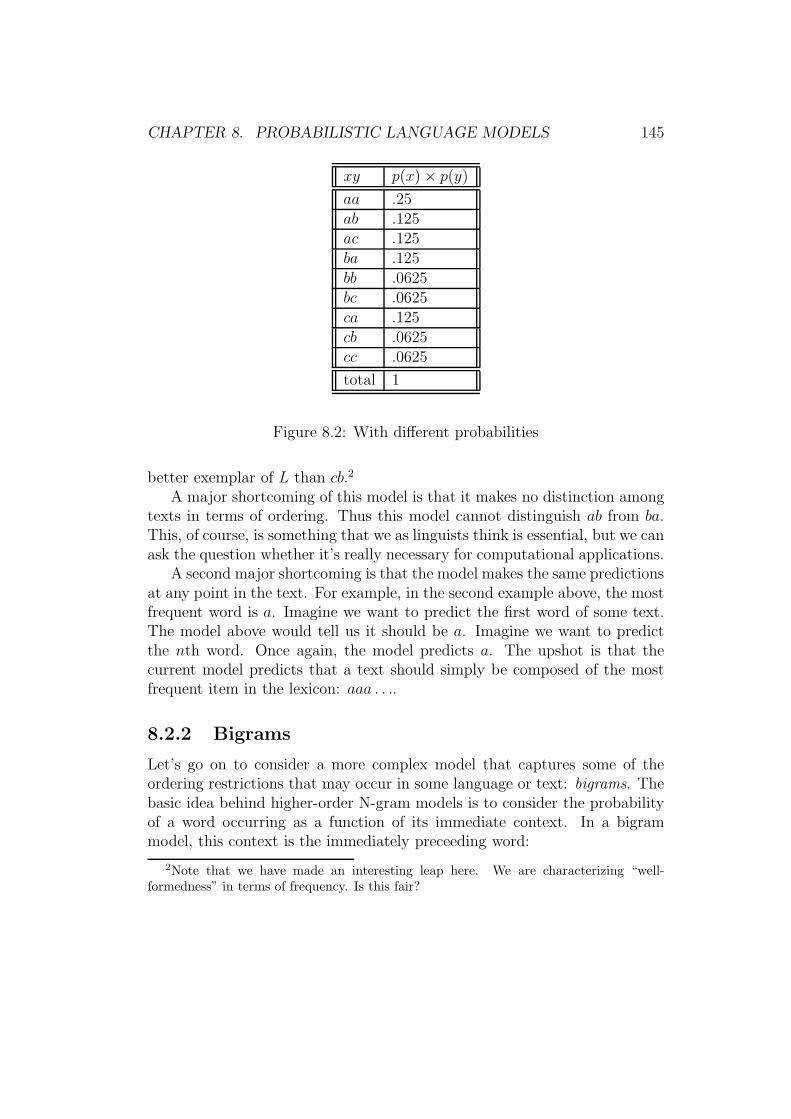
This is also the case if the individual words exhibit an asymmetric distri-bution. Assume a vocabulary with the same words, but where the individualword probabilities are different, i.e. p(a) = .5, p(b) = .25, and p(c) = .25(Table 8.2). The way this model works is that the well-formedness of a textfragment is correlated with its overall probability. Higher-probability textfragments are more well-formed than lower-probability texts, e.g. aa is a
CHAPTER 8. PROBABILISTIC LANGUAGE MODELS 145
xy p(x) × p(y)
aa .25ab .125ac .125ba .125bb .0625bc .0625ca .125cb .0625cc .0625
total 1
Figure 8.2: With different probabilities
better exemplar of L than cb.2
A major shortcoming of this model is that it makes no distinction amongtexts in terms of ordering. Thus this model cannot distinguish ab from ba.This, of course, is something that we as linguists think is essential, but we canask the question whether it’s really necessary for computational applications.
A second major shortcoming is that the model makes the same predictionsat any point in the text. For example, in the second example above, the mostfrequent word is a. Imagine we want to predict the first word of some text.The model above would tell us it should be a. Imagine we want to predictthe nth word. Once again, the model predicts a. The upshot is that thecurrent model predicts that a text should simply be composed of the mostfrequent item in the lexicon: aaa . . ..
8.2.2 Bigrams
Let’s go on to consider a more complex model that captures some of theordering restrictions that may occur in some language or text: bigrams. Thebasic idea behind higher-order N-gram models is to consider the probabilityof a word occurring as a function of its immediate context. In a bigrammodel, this context is the immediately preceeding word:
2Note that we have made an interesting leap here. We are characterizing “well-formedness” in terms of frequency. Is this fair?

CHAPTER 8. PROBABILISTIC LANGUAGE MODELS 146
(8.4) p(w1w2 . . . wi) = p(w1) × p(w2|w1) × . . . × p(wi|wi−1)
We calculate conditional probability in the usual fashion. (We use absolutevalue notation to denote the number of instances of some element.)
(8.5) p(wi|wi−1) =|wi−1wi|
|wi−1|
It’s important to notice that this is not the Chain Rule; here the context forthe conditional probabilities is the immediate context, not the whole context.As a consequence we cannot return to the joint probability algebraically, aswe did at the end of the preceding section (equation 8.2 on page 143). Wewill see that this limit on the context for the conditional probabilities in ahigher-order N-gram model has important consequences for how we mightactually manipulate such models computationally.
Let’s work out the bigrams in our tongue twister (repeated here).
Peter Piper picked a peck of pickled pepper.Where’s the pickled pepper that Peter Piper picked?
The frequency of the individual words is as in Table 8.3. The bigram fre-quencies are as in Table 8.4. Calculating conditional probabilities is then astraightforward matter of division. For example, the conditional probabilityof “Piper” given “Peter”:
(8.6) p(Piper|Peter) =|Peter Piper|
|Peter|=
2
2= 1
However, the conditional probability of “Piper” given “a”:
(8.7) p(Piper|a) =|a Piper|
|a|=
0
1= 0
Using conditional probabilities thus captures the fact that the likelihood of“Piper” varies by preceeding context: it is more likely after “Peter” thanafter “a”.

CHAPTER 8. PROBABILISTIC LANGUAGE MODELS 147
Word Frequency
Peter 2Piper 2
picked 2a 1
peck 1of 1
pickled 2pepper 2
Where’s 1the 1
that 1
Figure 8.3: Tongue twister frequencies
Bigrams Bigram frequencies
picked a 1pepper that 1
peck of 1a peck 1
pickled pepper 2Where s 1
Piper picked 2the pickled 1Peter Piper 2
of pickled 1pepper Where 1
that Peter 1s the 1
Figure 8.4: Twister bigram frequencies

CHAPTER 8. PROBABILISTIC LANGUAGE MODELS 148
The bigram model addresses both of the problems we identified with theunigram model above. First, recall that the unigram model could not distin-guish among different orderings. Different orderings are distinguished in thebigram model. Consider, for example, the difference between “Peter Piper”and “Piper Peter”. We’ve already seen that the former has a conditionalprobability of 1. The latter, on the other hand:
(8.8) p(Peter|Piper) =|Piper Peter|
|Piper|=
0
2= 0
The unigram model also made the prediction that the most well-formedtext should be composed of repetitions of the highest-probability items. Thebigram model excludes this possibility as well. Contrast the conditionalprobability of “Peter Piper” with “Peter Peter”:
(8.9) p(Peter|Peter) =|Peter Peter|
|Peter|=
0
2= 0
The bigram model presented doesn’t actually give a probability distri-bution for a string or sentence without adding something for the edges ofsentences. To get a correct probability distribution for the set of possiblesentences generated from some text, we must factor in the probability thatsome word begins the sentence, and that some word ends the sentence. Todo this, we define two markers that delimit all sentences: <s> and </s>.This transforms our text as follows.
<s> Peter Piper picked a peck of pickled pepper. </s><s> Where’s the pickled pepper that Peter Piper picked? </s>
Thus the probability of some sentence w1w2 . . . wn is given as:
(8.10) p(w1|<s>) × p(w2|w1) × . . . × p(</s>|wn)
Given the very restricted size of this text, and the conditional probabilitiesdependent on the newly added edge markers, there are only several specificways to add acceptable strings without reducing the probabilities to zero.Given the training text, these have the probabilities given below:
CHAPTER 8. PROBABILISTIC LANGUAGE MODELS 149
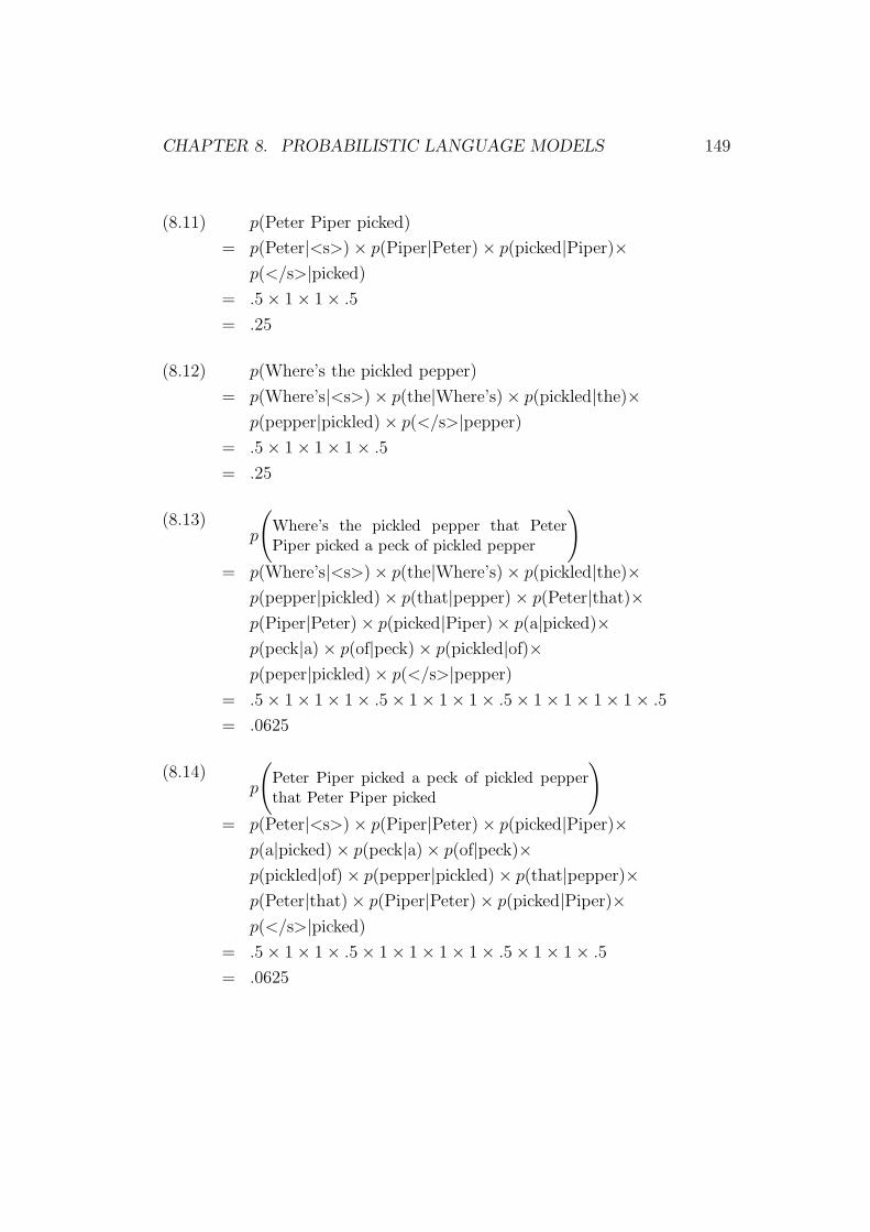
(8.11) p(Peter Piper picked)
= p(Peter|<s>) × p(Piper|Peter) × p(picked|Piper)×
p(</s>|picked)
= .5 × 1 × 1 × .5
= .25
(8.12) p(Where’s the pickled pepper)
= p(Where’s|<s>) × p(the|Where’s) × p(pickled|the)×
p(pepper|pickled) × p(</s>|pepper)
= .5 × 1 × 1 × 1 × .5
= .25
(8.13)p
(
Where’s the pickled pepper that PeterPiper picked a peck of pickled pepper
)
= p(Where’s|<s>) × p(the|Where’s) × p(pickled|the)×
p(pepper|pickled) × p(that|pepper) × p(Peter|that)×
p(Piper|Peter) × p(picked|Piper) × p(a|picked)×
p(peck|a) × p(of|peck) × p(pickled|of)×
p(peper|pickled) × p(</s>|pepper)
= .5 × 1 × 1 × 1 × .5 × 1 × 1 × 1 × .5 × 1 × 1 × 1 × 1 × .5
= .0625
(8.14)p
(
Peter Piper picked a peck of pickled pepperthat Peter Piper picked
)
= p(Peter|<s>) × p(Piper|Peter) × p(picked|Piper)×
p(a|picked) × p(peck|a) × p(of|peck)×
p(pickled|of) × p(pepper|pickled) × p(that|pepper)×
p(Peter|that) × p(Piper|Peter) × p(picked|Piper)×
p(</s>|picked)
= .5 × 1 × 1 × .5 × 1 × 1 × 1 × 1 × .5 × 1 × 1 × .5
= .0625

CHAPTER 8. PROBABILISTIC LANGUAGE MODELS 150
Notice how the text that our bigram frequencies were calculated on onlyleaves very restricted “choice” points. There are really only four:
1. What is the first word of the sentence: “Peter” or “Where’s”?
2. What is the last word of the sentence: “pepper” or “picked”?
3. What follows the word “picked”: “a” or </s>”?
4. What follows the word “pepper”: “that” or </s>?
The only sequences of words allowed are those sequences that occur in thetraining text. However, even with these restrictions, this allows for sentencesof unbounded length; an example like 8.14 can be extended infinitely.
Notice, however, that these restrictions do not guarantee that all sen-tences produced in conformity with this language model will be grammatical(by normal standards); example (8.13) is ungrammatical. Since the onlydependencies captured in a bigram model are local/immediate ones, suchsentences will emerge as well-formed.3
8.2.3 Higher-order N-grams
N-gram models are not restricted to unigrams and bigrams; higher-order N-gram models are also used. These higher-order models are characterized as wewould expect. For example, a trigram model would view a text w1w2 . . . wn
as the product of a series of conditional probabilities:
(8.15) p(w1w2 . . . wn) = p(w1) × p(w2|w1) ×∏
p(wn|wn−2wn−1)
8.2.4 N-gram approximation
One way to try to appreciate the success of N-gram language models is to usethem to approximate text in a generative fashion. That is, we can computeall the occurring N-grams over some text, and then use those N-grams togenerate new text.4
3Notice too, of course, that very simple sentences compatible with the vocabulary ofthis text would receive a null probability, e.g. “Where’s the pepper?” or “Peter picked apeck”, etc.
4See Shannon (1951).
CHAPTER 8. PROBABILISTIC LANGUAGE MODELS 151
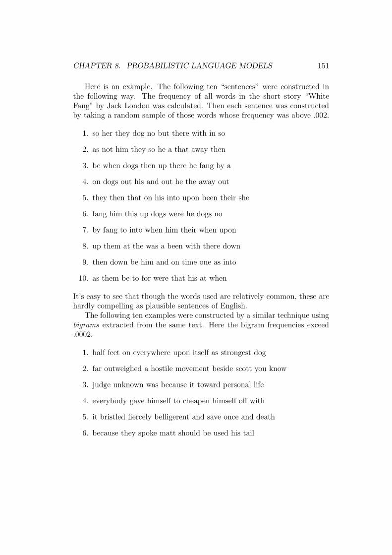
Here is an example. The following ten “sentences” were constructed inthe following way. The frequency of all words in the short story “WhiteFang” by Jack London was calculated. Then each sentence was constructedby taking a random sample of those words whose frequency was above .002.
1. so her they dog no but there with in so
2. as not him they so he a that away then
3. be when dogs then up there he fang by a
4. on dogs out his and out he the away out
5. they then that on his into upon been their she
6. fang him this up dogs were he dogs no
7. by fang to into when him their when upon
8. up them at the was a been with there down
9. then down be him and on time one as into
10. as them be to for were that his at when
It’s easy to see that though the words used are relatively common, these arehardly compelling as plausible sentences of English.
The following ten examples were constructed by a similar technique usingbigrams extracted from the same text. Here the bigram frequencies exceed.0002.
1. half feet on everywhere upon itself as strongest dog
2. far outweighed a hostile movement beside scott you know
3. judge unknown was because it toward personal life
4. everybody gave himself to cheapen himself off with
5. it bristled fiercely belligerent and save once and death
6. because they spoke matt should be used his tail

CHAPTER 8. PROBABILISTIC LANGUAGE MODELS 152
7. turn ’m time i counted the horse up live
8. beast that cautiously it discovered an act of plenty
9. fatty’s gone before had thought in matt argued stubbornly
10. what evil that night was flying brands from weakness
Notice that this latter set of sentences is far more natural sounding.
8.3 Hidden Markov Models
In this section, we treat Hidden Markov Models (HMMs). These are inti-mately associated with N-gram models and widely used as a computationalmodel for language processing.
8.3.1 Markov Chains
To understand Hidden Markov Models, we must first understand Markov
chains. These are basically DFAs with associated probabilities. Each arc isassociated with a probability value and all arcs leaving any particular nodemust exhibit a probability distribution, i.e. their values must range between 0and 1, and must total 1. In addition, one node is designated as the “starting”node.5 A simple example is given below.
(8.16)
s1
a .3
s2
b .7
a .2
b .8
As with an FSA, the machine moves from state to state following the arcsgiven. The sequence of arc symbols denotes the string generated—accepted—by the machine. The difference between a Markov chain and an FSA is that
5It’s not clear whether there is a set F of final states or if any state is a final state.The probability values associated with arcs do the work of selecting a final state.
CHAPTER 8. PROBABILISTIC LANGUAGE MODELS 153
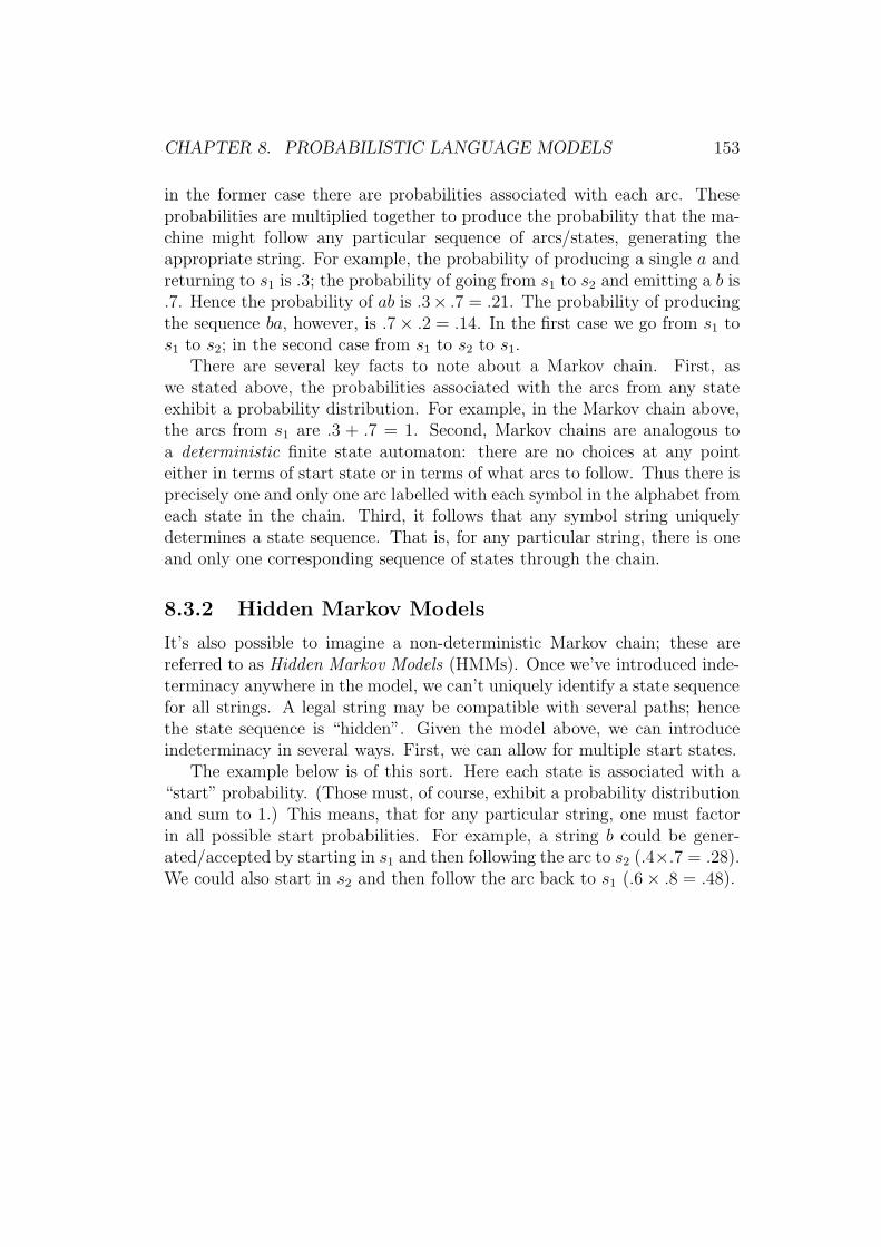
in the former case there are probabilities associated with each arc. Theseprobabilities are multiplied together to produce the probability that the ma-chine might follow any particular sequence of arcs/states, generating theappropriate string. For example, the probability of producing a single a andreturning to s1 is .3; the probability of going from s1 to s2 and emitting a b is.7. Hence the probability of ab is .3× .7 = .21. The probability of producingthe sequence ba, however, is .7 × .2 = .14. In the first case we go from s1 tos1 to s2; in the second case from s1 to s2 to s1.
There are several key facts to note about a Markov chain. First, aswe stated above, the probabilities associated with the arcs from any stateexhibit a probability distribution. For example, in the Markov chain above,the arcs from s1 are .3 + .7 = 1. Second, Markov chains are analogous toa deterministic finite state automaton: there are no choices at any pointeither in terms of start state or in terms of what arcs to follow. Thus there isprecisely one and only one arc labelled with each symbol in the alphabet fromeach state in the chain. Third, it follows that any symbol string uniquelydetermines a state sequence. That is, for any particular string, there is oneand only one corresponding sequence of states through the chain.
8.3.2 Hidden Markov Models
It’s also possible to imagine a non-deterministic Markov chain; these arereferred to as Hidden Markov Models (HMMs). Once we’ve introduced inde-terminacy anywhere in the model, we can’t uniquely identify a state sequencefor all strings. A legal string may be compatible with several paths; hencethe state sequence is “hidden”. Given the model above, we can introduceindeterminacy in several ways. First, we can allow for multiple start states.
The example below is of this sort. Here each state is associated with a“start” probability. (Those must, of course, exhibit a probability distributionand sum to 1.) This means, that for any particular string, one must factorin all possible start probabilities. For example, a string b could be gener-ated/accepted by starting in s1 and then following the arc to s2 (.4×.7 = .28).We could also start in s2 and then follow the arc back to s1 (.6 × .8 = .48).

CHAPTER 8. PROBABILISTIC LANGUAGE MODELS 154
(8.17)
s1 .4
a .3
s2 .6
b .7
a .2
b .8
The overall probability of the string b is the sum of the probabilities ofall possible paths through the HMM: .28 + .48 = .76. Notice then that wecannot really be sure which path may have been taken to get to b, though ifthe paths have different probabilities then we can calculate the most likelypath. In the case at hand, this is s2 ⊢ s1.
Indeterminacy can also be introduced by adding multiple arcs from thesame state for the same symbol. For example, the HMM below is a minimalmodification of the Markov chain above.
(8.18)
s1
a .3
s2
a .2
b .5
a .2
b .8
Consider how this HMM deals with a string ab. Here only s1 is a legal startstate. We can generate/accept a by either following the arc back to s1 (.3) orby following the arc to s2 (.2). In the former case, we can get b by following

CHAPTER 8. PROBABILISTIC LANGUAGE MODELS 155
the arc from s1 to s2. In the latter case, we can get b by following the arcfrom s2 back to s1. This gives the following total probabilities for the twostate sequences given.
(8.19) s1 ⊢ s1 ⊢ s2 = .3 × .5 = .15
s1 ⊢ s2 ⊢ s1 = .2 × .8 = .16
This results in an overall probability of .31 for ab. The second state sequenceis of course the more likely one since it exhibits a higher overall probability.
A HMM can naturally include both extra arcs and multiple start states.The HMM below exemplifies.
(8.20)
s1 .1
a .3
s2 .9
a .2
b .5
a .2
b .8
This generally results in even more choices for any particular string. Forexample, the string ab can be produced with all the following sequences:
(8.21) s1 ⊢ s1 ⊢ s2 = .1 × .3 × .5 = .015
s1 ⊢ s2 ⊢ s1 = .1 × .2 × .8 = .016
s2 ⊢ s1 ⊢ s2 = .9 × .2 × .5 = .09
The overall probability is then .121.
CHAPTER 8. PROBABILISTIC LANGUAGE MODELS 156
8.3.3 Formal HMM properties
There are a number of formal properties of Markov chains and HMMs thatare useful. One extremely important property is Limited Horizon:
(8.22) p(Xt+1 = sk|X1, . . . , Xt) = p(Xt+1 = sk|Xt)
This says that the probability of some state sk given the set of states thathave occurred before it is the same as the probability of that state given thesingle state that occurs just before it.
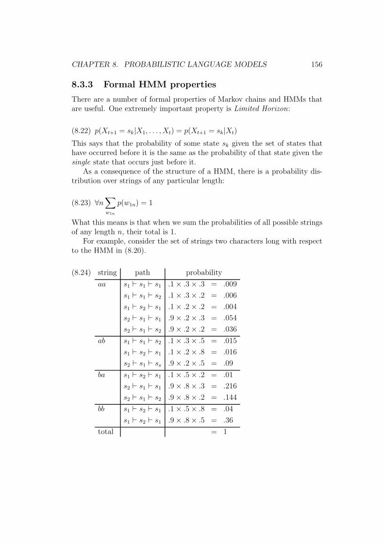
As a consequence of the structure of a HMM, there is a probability dis-tribution over strings of any particular length:
(8.23) ∀n∑
w1n
p(w1n) = 1
What this means is that when we sum the probabilities of all possible stringsof any length n, their total is 1.
For example, consider the set of strings two characters long with respectto the HMM in (8.20).
(8.24) string path probability
aa s1 ⊢ s1 ⊢ s1 .1 × .3 × .3 = .009
s1 ⊢ s1 ⊢ s2 .1 × .3 × .2 = .006
s1 ⊢ s2 ⊢ s1 .1 × .2 × .2 = .004
s2 ⊢ s1 ⊢ s1 .9 × .2 × .3 = .054
s2 ⊢ s1 ⊢ s2 .9 × .2 × .2 = .036
ab s1 ⊢ s1 ⊢ s2 .1 × .3 × .5 = .015
s1 ⊢ s2 ⊢ s1 .1 × .2 × .8 = .016
s2 ⊢ s1 ⊢ ss .9 × .2 × .5 = .09
ba s1 ⊢ s2 ⊢ s1 .1 × .5 × .2 = .01
s2 ⊢ s1 ⊢ s1 .9 × .8 × .3 = .216
s2 ⊢ s1 ⊢ s2 .9 × .8 × .2 = .144
bb s1 ⊢ s2 ⊢ s1 .1 × .5 × .8 = .04
s1 ⊢ s2 ⊢ s1 .9 × .8 × .5 = .36
total = 1
CHAPTER 8. PROBABILISTIC LANGUAGE MODELS 157
8.3.4 Bigrams and HMMs
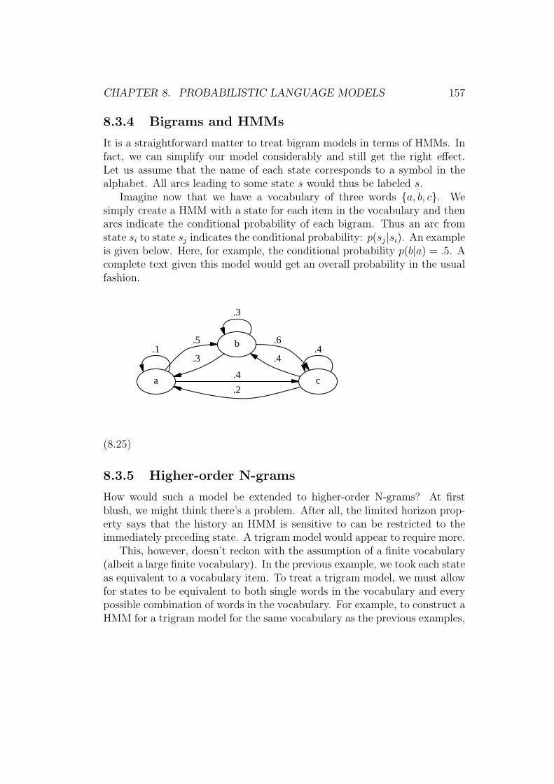
It is a straightforward matter to treat bigram models in terms of HMMs. Infact, we can simplify our model considerably and still get the right effect.Let us assume that the name of each state corresponds to a symbol in thealphabet. All arcs leading to some state s would thus be labeled s.
Imagine now that we have a vocabulary of three words {a, b, c}. Wesimply create a HMM with a state for each item in the vocabulary and thenarcs indicate the conditional probability of each bigram. Thus an arc fromstate si to state sj indicates the conditional probability: p(sj |si). An exampleis given below. Here, for example, the conditional probability p(b|a) = .5. Acomplete text given this model would get an overall probability in the usualfashion.
(8.25)
a
.1b.5
c.4
.3
.3
.6
.2
.4.4
8.3.5 Higher-order N-grams
How would such a model be extended to higher-order N-grams? At firstblush, we might think there’s a problem. After all, the limited horizon prop-erty says that the history an HMM is sensitive to can be restricted to theimmediately preceding state. A trigram model would appear to require more.
This, however, doesn’t reckon with the assumption of a finite vocabulary(albeit a large finite vocabulary). In the previous example, we took each stateas equivalent to a vocabulary item. To treat a trigram model, we must allowfor states to be equivalent to both single words in the vocabulary and everypossible combination of words in the vocabulary. For example, to construct aHMM for a trigram model for the same vocabulary as the previous examples,
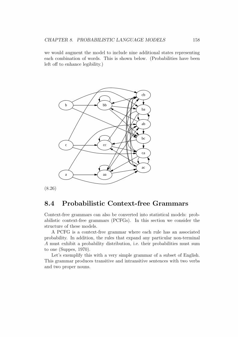
CHAPTER 8. PROBABILISTIC LANGUAGE MODELS 158
we would augment the model to include nine additional states representingeach combination of words. This is shown below. (Probabilities have beenleft off to enhance legibility.)
(8.26)
a aa
ab
ac
babb
bc
ca
cb
cc
b
c
8.4 Probabilistic Context-free Grammars
Context-free grammars can also be converted into statistical models: prob-abilistic context-free grammars (PCFGs). In this section we consider thestructure of these models.
A PCFG is a context-free grammar where each rule has an associatedprobability. In addition, the rules that expand any particular non-terminalA must exhibit a probability distribution, i.e. their probabilities must sumto one (Suppes, 1970).
Let’s exemplify this with a very simple grammar of a subset of English.This grammar produces transitive and intransitive sentences with two verbsand two proper nouns.
CHAPTER 8. PROBABILISTIC LANGUAGE MODELS 159
(8.27) S → NP V P
V P → V
V P → V NP
V → sees
V → helps
NP → Mindy
NP → Mary
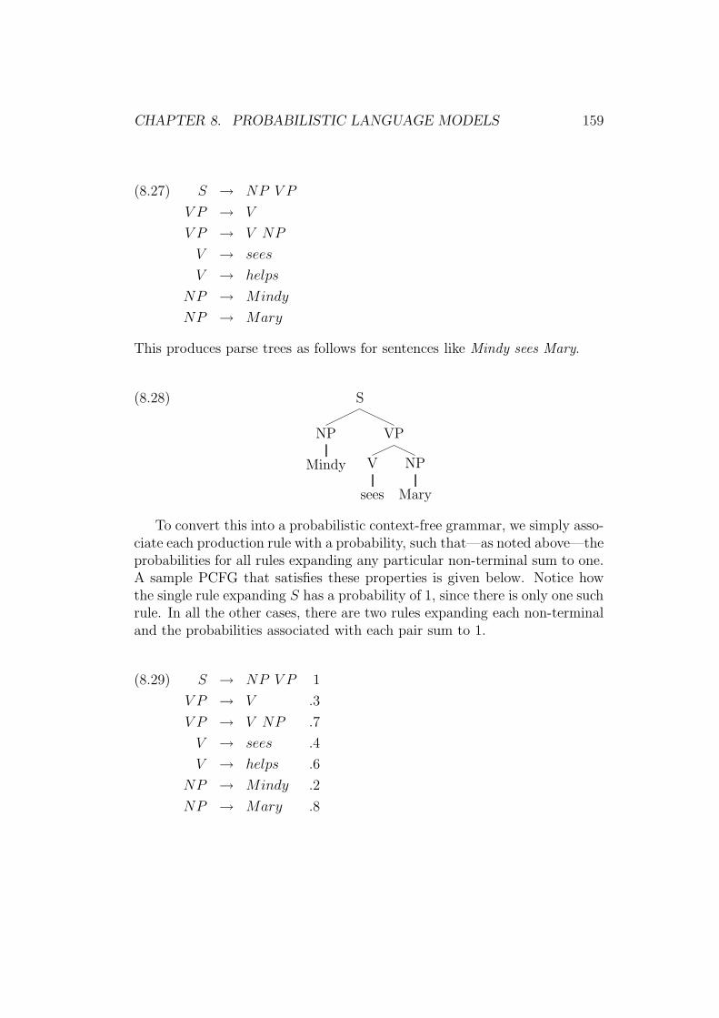
This produces parse trees as follows for sentences like Mindy sees Mary.
(8.28) S
NP
Mindy
VP
V
sees
NP
Mary
To convert this into a probabilistic context-free grammar, we simply asso-ciate each production rule with a probability, such that—as noted above—theprobabilities for all rules expanding any particular non-terminal sum to one.A sample PCFG that satisfies these properties is given below. Notice howthe single rule expanding S has a probability of 1, since there is only one suchrule. In all the other cases, there are two rules expanding each non-terminaland the probabilities associated with each pair sum to 1.
(8.29) S → NP V P 1
V P → V .3
V P → V NP .7
V → sees .4
V → helps .6
NP → Mindy .2
NP → Mary .8

CHAPTER 8. PROBABILISTIC LANGUAGE MODELS 160
The probability of some parse of a sentence is then the product of theprobabilities of all the rules used.6 In the example at hand, Mindy sees Mary,we get: 1 × .2 × .7 × .4 × .8 = .0448. The probability of a sentence s, e.g.any particular string of words, is the sum of the probabilities of all its parsest1, t2, . . . , tn.
(8.30) p(s) =∑
j
p(tj)p(s|tj)
In the case at hand, there are no structural ambiguities; there is only onepossible structure for any acceptable sentence. Let’s consider another ex-ample, but one where there are structural ambiguities. The very simplifiedcontext-free grammar for noun conjunction below has these properties.
(8.31) NP → NP C NP .4
NP → Mary .3
NP → Mindy .2
NP → Mark .1
C → and 1
This grammar results in multiple trees for conjoined nouns like Mary
and Mindy and Mark as below. The ambiguity surrounds whether the firsttwo conjuncts are grouped together or the last two. The same rules areused in each parse, so the probability of either one of them is: .3 × .2 ×.1 × 1 × 1 × .4 × .4 = .00096. The overall probability of the string is then.00096 + .00096 = .00192.
6Note that if any rule is used more than once then it’s probability is factored in asmany times as it is used.
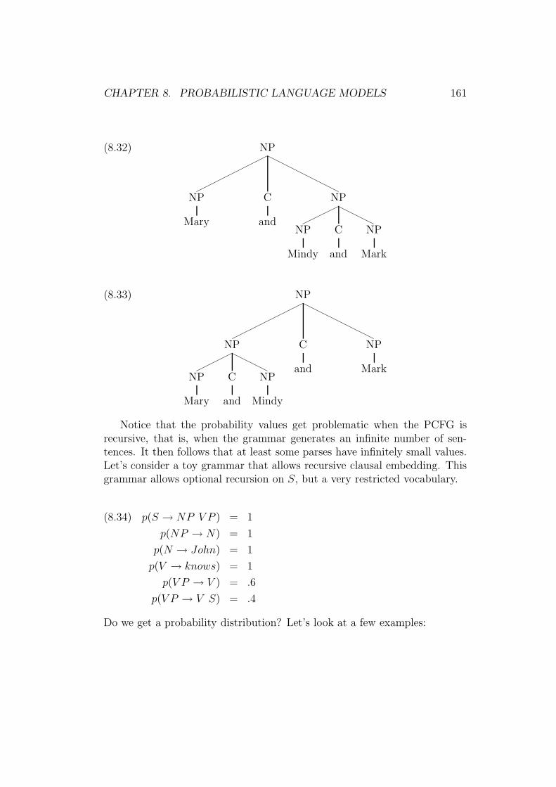
CHAPTER 8. PROBABILISTIC LANGUAGE MODELS 161
(8.32) NP
NP
Mary
C
and
NP
NP
Mindy
C
and
NP
Mark
(8.33) NP
NP
NP
Mary
C
and
NP
Mindy
C
and
NP
Mark
Notice that the probability values get problematic when the PCFG isrecursive, that is, when the grammar generates an infinite number of sen-tences. It then follows that at least some parses have infinitely small values.Let’s consider a toy grammar that allows recursive clausal embedding. Thisgrammar allows optional recursion on S, but a very restricted vocabulary.
(8.34) p(S → NP V P ) = 1
p(NP → N) = 1
p(N → John) = 1
p(V → knows) = 1
p(V P → V ) = .6
p(V P → V S) = .4
Do we get a probability distribution? Let’s look at a few examples:

CHAPTER 8. PROBABILISTIC LANGUAGE MODELS 162
(8.35) S
NP
N
John
VP
V
knows
We have p(John knows) = 1 × 1 × 1 × .6 × 1 = .6
(8.36) S
NP
N
John
VP
V
knows
S
NP
N
John
VP
V
knows
We have p(John knows John knows) = 1×1×1×.4×1×1×1×1×.6×1 = .24.
CHAPTER 8. PROBABILISTIC LANGUAGE MODELS 163
(8.37) S
NP
N
John
VP
V
knows
S
NP
N
John
VP
V
knows
S
NP
N
John
VP
V
knows
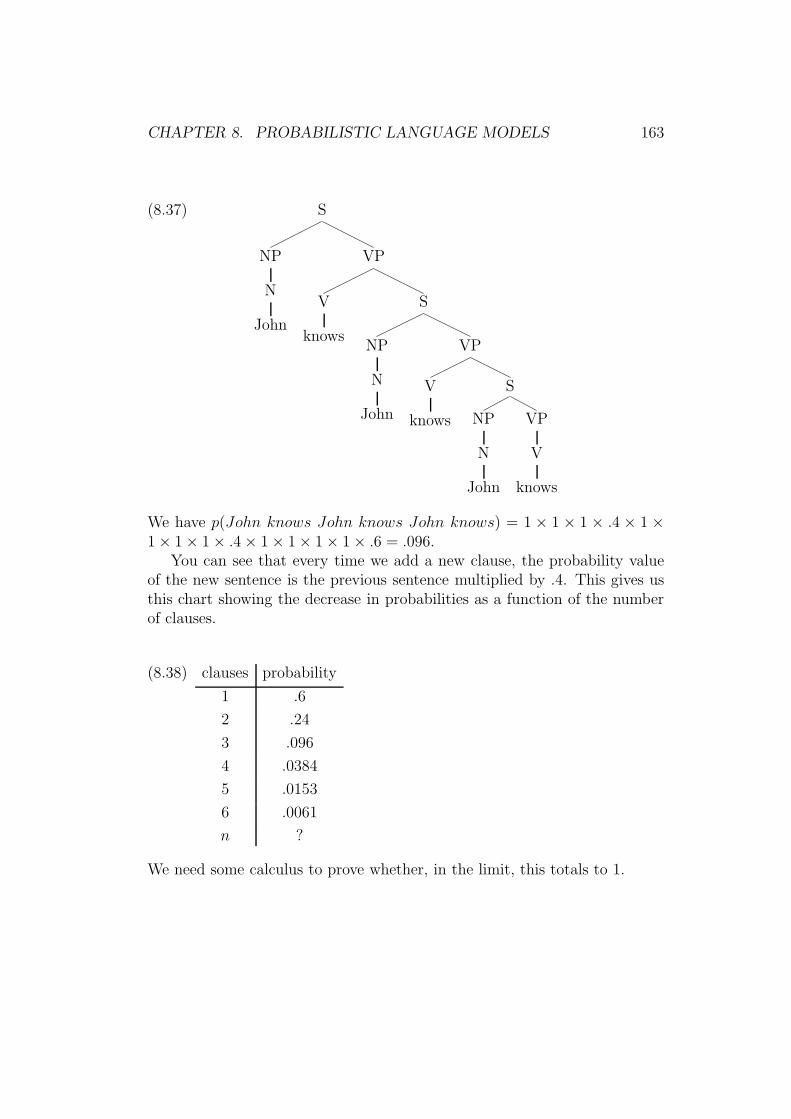
We have p(John knows John knows John knows) = 1 × 1 × 1 × .4 × 1 ×1 × 1 × 1 × .4 × 1 × 1 × 1 × 1 × .6 = .096.
You can see that every time we add a new clause, the probability valueof the new sentence is the previous sentence multiplied by .4. This gives usthis chart showing the decrease in probabilities as a function of the numberof clauses.
(8.38) clauses probability
1 .6
2 .24
3 .096
4 .0384
5 .0153
6 .0061
n ?
We need some calculus to prove whether, in the limit, this totals to 1.

CHAPTER 8. PROBABILISTIC LANGUAGE MODELS 164
Chi (1999) shows formally that PCFGs don’t exhibit a probability dis-tribution. He argues as follows. FIrst, assume a grammar with only tworules:
(8.39) S → S S
S → a
If p(S → S S) = n then p(S → a) = 1−n. Chi argues as follows: “Let xh bethe total probability of all parses with height no larger than h. Clearly, xh
is increasing. It is not hard to see that xh+l = (1− n) + nx2h. Therefore, the
limit of xh, which is the total probability of all parses, is a solution for theequation x = (1− n) + nx2. The equation has two solutions: 1 and 1
n− 1. It
can be shown that x is the smaller of the two: x = min(1, 1n− 1). Therefore,
if n > 12, x < 1—an improper probability.”
8.5 Summary
This chapter links the ideas about probability from the preceding chapterwith the notions of grammar and automaton developed earlier.
We began with the notion of N-gram modeling. The basic idea is that wecan view a strings of words or symbols in terms of the likelihood that eachword might follow the preceding one or two words. While this is a stagger-ingly simple idea, it actually can go quite some distance toward describingnatural language data.
We next turned to Markov Chains and Hidden Markov Models (HMMs).These are probabilistically weighted finite state devices and can be used toassociate probabilities with FSAs.
We showed in particular how a simplified Markov Model could be used toimplement N-grams, showing that those models could be treated in restrictiveterms.
Finally, we very briefly considered probabilistic context-free grammars.
8.6 Exercises
None yet.