Chapter 8 Numerical Techniques - rsmith.math.ncsu.edu
37
“book” 2008/1/15 page 373 ✐ ✐ ✐ ✐ ✐ ✐ ✐ ✐ Chapter 8 Numerical Techniques The rod, beam, plate and shell models developed in Chapter 7 generally preclude analytic solution due to the boundary conditions and piecewise nature of material parameters and exogenous inputs. This necessitates the development of approxima- tion techniques appropriate not only for simulations and transducer characterization but also for optimization and control design. Whereas we focus primarily on the first objective in this chapter, the use of these numerical models for subsequent trans- ducer optimization and control design dictates that attention be paid to additional criteria, such as adjoint convergence, that arise in the context of constrained opti- mization — the reader is referred to [67] and references therein for details regarding approximation techniques pertaining to optimization and control formulations. For all of the models, we first employ Galerkin approximations in space to obtain semi-discrete, vector-valued ODE that evolve in time — see pages 417–419 of Appendix A for a general discussion regarding the relation between Galerkin and finite element methods. This provides a natural setting for linear and nonlinear finite-dimensional control design and direct simulations. Since Galerkin or finite element approximation in space typically yield moderately stiff ODE systems, A- stable or stiff algorithms are advised when approximating solutions in time; this includes trapezoidal-based approximations or routines such as ode15s.m in MAT- LAB. In all cases, we consider approximation in the context of the weak model formulations since this reduces smoothness requirements and accommodates in a natural manner discontinuous material parameters and inputs. This necessarily involves the integration of polynomial or trigonometric basis elements which we accomplish using Gaussian quadrature routines chosen to ensure exact integration for linear and cubic basis functions. We summarize these numerical integration algorithms in Section 8.1. Approximation techniques for rods, beams, plates and shells are subsequently described in Section 8.2–8.5. Numerical approximation of distributed structural models is an extremely broad topic and includes issues such as shear locking and approximation techniques for control design which constitute active research areas. Rather than attempt to 373
Transcript of Chapter 8 Numerical Techniques - rsmith.math.ncsu.edu
“book”2008/1/15page 373
i
i
i
i
i
i
i
i
Chapter 8
Numerical Techniques
The rod, beam, plate and shell models developed in Chapter 7 generally precludeanalytic solution due to the boundary conditions and piecewise nature of materialparameters and exogenous inputs. This necessitates the development of approxima-tion techniques appropriate not only for simulations and transducer characterizationbut also for optimization and control design. Whereas we focus primarily on the firstobjective in this chapter, the use of these numerical models for subsequent trans-ducer optimization and control design dictates that attention be paid to additionalcriteria, such as adjoint convergence, that arise in the context of constrained opti-mization — the reader is referred to [67] and references therein for details regardingapproximation techniques pertaining to optimization and control formulations.
For all of the models, we first employ Galerkin approximations in space toobtain semi-discrete, vector-valued ODE that evolve in time — see pages 417–419of Appendix A for a general discussion regarding the relation between Galerkin andfinite element methods. This provides a natural setting for linear and nonlinearfinite-dimensional control design and direct simulations. Since Galerkin or finiteelement approximation in space typically yield moderately stiff ODE systems, A-stable or stiff algorithms are advised when approximating solutions in time; thisincludes trapezoidal-based approximations or routines such as ode15s.m in MAT-LAB.
In all cases, we consider approximation in the context of the weak modelformulations since this reduces smoothness requirements and accommodates in anatural manner discontinuous material parameters and inputs. This necessarilyinvolves the integration of polynomial or trigonometric basis elements which weaccomplish using Gaussian quadrature routines chosen to ensure exact integrationfor linear and cubic basis functions. We summarize these numerical integrationalgorithms in Section 8.1. Approximation techniques for rods, beams, plates andshells are subsequently described in Section 8.2–8.5.
Numerical approximation of distributed structural models is an extremelybroad topic and includes issues such as shear locking and approximation techniquesfor control design which constitute active research areas. Rather than attempt to
373

“book”2008/1/15page 374
i
i
i
i
i
i
i
i
374 Chapter 8. Numerical Techniques
provide a comprehensive description of numerical techniques, we instead summa-rize certain fundamental methods appropriate for smart structures and indicatepitfalls and directions required to extend the algorithms to more complex settings.The reader is referred to [54, 479] for finite element theory, [390, 462, 527] for finiteelement implementation techniques, and [163, 383, 406] for the theory of splines,variational methods and Galerkin techniques. A detailed discussion illustratingfinite element implementation in MATLAB is provided in [276] and m-files for im-plementing various models discussed in this chapter are provided at the websitehttp://www.siam.org/books/fr32. Additional references specific to the variousstructures will be indicated in relevant sections.
8.1 Quadrature Techniques
Consider integrals of the form I =∫ b
a f(x)dx where (a, b) is either finite or infiniteand the value I is finite. The goal in numerical integration or quadrature is toapproximate I by finite sums of the form
In =
n∑
i=0
wif(xi)
where wi and xi respectively denote quadrature weights and nodes. Various ap-proximation theories — e.g., based on Taylor expansions or the theory of orthogo-nal polynomials — yield choices for wi and xi that determine the rate at which In
converges to I as n → ∞.
8.1.1 Newton–Cotes Formulae
To illustrate issues associated with the choice of weights and nodes, we considerfirst closed and open Newton–Cotes formulae for finite [a, b]. The nodes for the twocases are xi = x0 + ih where i = 0, . . . , n and
h =b − a
n, x0 = a, closed Newton–Cotes formulae
h =b − a
n + 2, x0 = a + h, open Newton–Cotes formulae.
Hence nodes lie in the closed interval [a, b] in the first case and the open interval (a, b)in the second. In all of the following formulae, ξ is a point in (a, b) and f is assumedsufficiently smooth so that requisite derivatives exist and are continuous. Detailsregarding the derivation of these relations can be found in [19]. The trapezoid andmidpoint rules are illustrated in Figure 8.1.
Closed Newton–Cotes Formulae
1. (n = 1) Trapezoidal rule
∫ b
a
f(x)dx =h
2[f(x0) + f(x1)] −
h3
12f ′′(ξ) (8.1)

“book”2008/1/15page 375
i
i
i
i
i
i
i
i
8.1. Quadrature Techniques 375
ba(a)
a b(b)
Figure 8.1. (a) Trapezoidal rule and (b) midpoint rule for the interval [a, b].
2. (n = 2) Simpson’s rule
∫ b
a
f(x)dx =h
3[f(x0) + 4f(x1) + f(x2)] −
h5
90f (4)(ξ) (8.2)
3. (n = 3) Simpson’s three-eighths rule
∫ b
a
f(x)dx =3h
8[f(x0) + 3f(x1) + 3f(x2) + f(x3)] −
3h5
80f (4)(ξ) (8.3)
4. (n = 4) Milne’s rule
∫ b
a
f(x)dx =2h
45[7f(x0)+32f(x1)+12f(x2)+32f(x3)+7f(x4)]−
8h7
945f (6)(ξ) (8.4)
Open Newton–Cotes Formulae
1. (n = 0) Midpoint rule
∫ b
a
f(x)dx = 2hf(x0) +h3
3f ′′(ξ) (8.5)
2. (n = 1) ∫ b
a
f(x)dx =3h
2[f(x0) + f(x1)] +
3h3
4f ′′(ξ) (8.6)
3. (n = 2)
∫ b
a
f(x)dx =4h
3[2f(x0) − f(x1) + 2f(x2)] +
14h5
45f (4)(ξ) (8.7)
4. (n = 3)
∫ b
a
f(x)dx =5h
24[11f(x0) + f(x1) + f(x2) + 11f(x3)] +
95h5
144f (4)(ξ) (8.8)
“book”2008/1/15page 376
i
i
i
i
i
i
i
i
376 Chapter 8. Numerical Techniques
Accuracy of the Newton–Cotes Formulae
A numerical quadrature formula In is said to have degree of precision m if In =I for all polynomials f such that deg(f) ≤ m and In 6= I for deg(f) = m+1. Hencethe trapezoid rule has degree of precision 1 which corroborates the observationthat it integrates linear polynomials exactly. It is observed that formulae withan even index gain an extra degree of precision when compared with odd formulaewhich often makes them preferable. For later comparison with Gaussian quadratureroutines, we note that the errors En and degrees of precision DPn for the Newton–Cotes formulae are
|En| =
K1nhn+2f (n+1)(ξ) , n odd
K2nhn+3f (n+2)(ξ) , n even
and
DPn =
n , n odd
n + 1 , n even
where K1n and K2n are constants and it is assumed that f ∈ Cn+2[a, b] if n is evenand f ∈ Cn+1[a, b] for odd n.
Whereas increasing n leads to improved accuracy, Newton–Cotes formulae aretypically restricted to n ≤ 8 to avoid stability issues. To achieve the requisite accu-racy on large intervals [a, b], including infinite intervals, alternatives are required.These include Romberg integration techniques which improve accuracy throughRichardson extrapolation, composite rules, and Gaussian quadrature techniques.We summarize next the latter two options.
Composite Quadrature Techniques
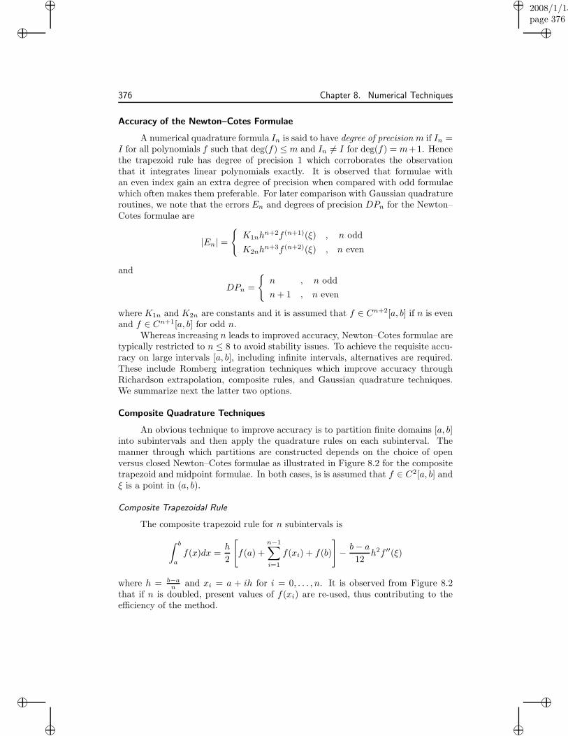
An obvious technique to improve accuracy is to partition finite domains [a, b]into subintervals and then apply the quadrature rules on each subinterval. Themanner through which partitions are constructed depends on the choice of openversus closed Newton–Cotes formulae as illustrated in Figure 8.2 for the compositetrapezoid and midpoint formulae. In both cases, is is assumed that f ∈ C2[a, b] andξ is a point in (a, b).
Composite Trapezoidal Rule
The composite trapezoid rule for n subintervals is
∫ b
a
f(x)dx =h
2
[f(a) +
n−1∑
i=1
f(xi) + f(b)
]− b − a
12h2f ′′(ξ)
where h = b−an and xi = a + ih for i = 0, . . . , n. It is observed from Figure 8.2
that if n is doubled, present values of f(xi) are re-used, thus contributing to theefficiency of the method.
“book”2008/1/15page 377
i
i
i
i
i
i
i
i
8.1. Quadrature Techniques 377
ba(a)
a b(b)
Figure 8.2. (a) Composite trapezoidal rule and (b) composite midpoint rule withthree subintervals.
Composite Midpoint Rule
The composite midpoint formula for even n and n2 + 1 subintervals is
∫ b
a
f(x)dx = 2h
n/2∑
i=0
f(xi) +b − a
6h2f ′′(ξ).
Here h = b−an+2 and xi = a + (2i + 1)h for i = 0, . . . , n. The approximation obtained
with n = 4, and hence 3 subintervals is illustrated in Figure 8.2(b).
8.1.2 Gaussian Quadrature Techniques
It is observed that for the open and closed Newton–Cotes formulae, and correspond-ing composite rules, the quadrature points xi are fixed a priori and quadratureweights wi are determined to achieve a specified level of accuracy. Hence both theaccuracy and degree of precision for the methods are roughly equivalent to the de-grees of freedom associated with the weights. Alternatively, one can let both xi andwi be free parameters to achieve a maximal order of accuracy. This is the basis forGaussian quadrature routines which provides the capability for exactly integratingpolynomials up to degree 2n− 1 using n-point expansions.
To provide intuition, we initially consider the expansion
∫ 1
−1
f(x)dx ≈n∑
i=1
f(xi)wi
with n = 1 and n = 2. Defining the error as
En(f) =
∫ 1
−1
f(x)dx −n∑
i=1
f(xi)wi,
we note that for polynomials pm = a0 + a1x + · · · + amxm,
En(pm) = a0En(1) + a1En(x) + · · · + amEn(xm).
It thus follows that the integration rule has degree of precision m if
En(xi) = 0 , i = 0, . . . , m.

“book”2008/1/15page 378
i
i
i
i
i
i
i
i
378 Chapter 8. Numerical Techniques
1-Point Gaussian Quadrature
To determine the two parameters x1 and w1, we consider the constraints
E1(1) = 0 , E1(x) = 0
or ∫ 1
−1
1dx − w1 = 0 ,
∫ 1
−1
xdx − w1x1 = 0.
This yields x1 = 0 and w1 = 2 and the general quadrature rule
∫ 1
−1
f(x)dx ≈ 2f(0).
Note that this is simply the midpoint formula (8.5) which is illustrated for theinterval [a, b] in Figure 8.1(b).
2-Point Gaussian Quadrature
Here there are four parameters x1, x2, w1, w2 and four constraints
E2(xi) =
∫ 1
−1
xidx − (w1xi1 + w2x
i2) = 0 , i = 0, 1, 2, 3.
This yields the nonlinear system of equations
w1 + w2 = 2
w1x1 + w2x2 = 0
w1x21 + w2x
22 =
2
3
w1x31 + w2x
32 = 0
which has the unique solution
x1 = − 1√3
, w1 = 1
x2 = 1√3
, w2 = 1.
It is noted that the general quadrature rule
∫ 1
−1
f(x)dx ≈ f
(−1√3
)+ f
(1√3
)(8.9)
has the same degree of precision as Simpson’s rule (8.2) which required three nodes.
n-Point Gaussian Quadrature
For n > 2, solving the nonlinear systems of equations becomes prohibitive andGaussian quadrature rules are typically formulated using interpolation theory for

“book”2008/1/15page 379
i
i
i
i
i
i
i
i
8.1. Quadrature Techniques 379
orthogonal polynomials. By considering families of orthogonal polynomials definedon the intervals [−1, 1], [0,∞) and (−∞,∞), in addition to weighted integrands,this provides substantial flexibility for approximating a broad range of integrals. Acomplete discussion of this theory is beyond the scope of this chapter and we referthe reader to [19, 125, 528] for details regarding Gaussian quadrature routines forboth single and multivariate approximation.
Gauss–Legendre Quadrature
Gauss–Legendre quadrature formulae are typically defined in terms of degree nLegendre polynomials
Pn(x) =1
2nn!· dn
dxn
(x2 − 1
)n, n = 0, 1, 2, . . .
on the interval [−1, 1] — see [123,465] for a derivation of the Legendre polynomialsthrough application of the Gram–Schmidt process to the sequence 1, x, x2, · · · . Notethat the first five Legendre polynomials are
P0(x) = 1
P1(x) = x
P2(x) =1
2(3x2 − 1)
P3(x) =1
2(5x3 − 3x)
P4(x) =1
8(35x4 − 30x2 + 3).
The quadrature relation is
∫ 1
−1
f(x)dx ≈n∑
i=1
wif(xi) (8.10)
where the nodes xi are zeroes of Pn(x) and the weights are
wi =−2
(n + 1)P ′n(xi)Pn+1(xi)
, i = 1, . . . , n,
as summarized in Table 8.1. For f ∈ C2n[−1, 1], the errors are given by
En(f) = enf (2n)(ξ)
(2n)!
where ξ is a point in [−1, 1] and en ≈ π4n as n → ∞ [19]. As noted previously, this
implies that the quadrature formula (8.10) is exact for polynomials having degreeless than or equal to 2n − 1. Hence when approximating the solution to weakformulations for structural models, the degree n is chosen to be commensurate withfinite element or spline basis and test functions.

“book”2008/1/15page 380
i
i
i
i
i
i
i
i
380 Chapter 8. Numerical Techniques
n Nodes xi Weights wi
1 0 2
2 ± 1√3
1
3 0 89
±√
35
59
4 ±√
15+2√
30√35
496(18+
√30)
±√
15−2√
30√35
496(18−
√30)
Table 8.1. Nodes and weights for Gauss–Legendre quadrature on [−1, 1].
Gauss–Laguerre and Gauss–Hermite Quadrature
The integrals in the polarization model (2.114) involve the domains [0,∞)and (−∞,∞). One technique for approximating the integrals is to exploit decayexhibited by the integrand to truncate to finite domains. Alternatively, one candirectly approximate the integrals using orthogonal polynomials defined on the halfline and real line. This yields the Gauss–Laguerre quadrature relation
∫ ∞
0
e−xf(x)dx ≈n∑
i=1
wif(xi)
and Gauss–Hermite relation
∫ ∞
−∞e−x2
f(x)dx ≈n∑
i=1
wif(xi).
The weights and nodes for these formulae can be found in [528].
Gauss–Legendre Quadrature on [a, b] and Composite Quadrature
To evaluate integrals on arbitrary domains using the Gauss–Legendre quadra-ture relation (8.10), one can employ the linear change of variables
∫ b
a
f(x)dx =b − a
2
∫ 1
−1
f
(a + b + ξ(b − a)
2
)dξ (8.11)
to map to the interval [−1, 1]. It follows that the nodes and weights xi and wi for[a, b] are related to ξi and ηi for [−1, 1] by the relations
xi =a + b
2+
b − a
2ξi , wi =
b − a
2ηi.
“book”2008/1/15page 381
i
i
i
i
i
i
i
i
8.1. Quadrature Techniques 381
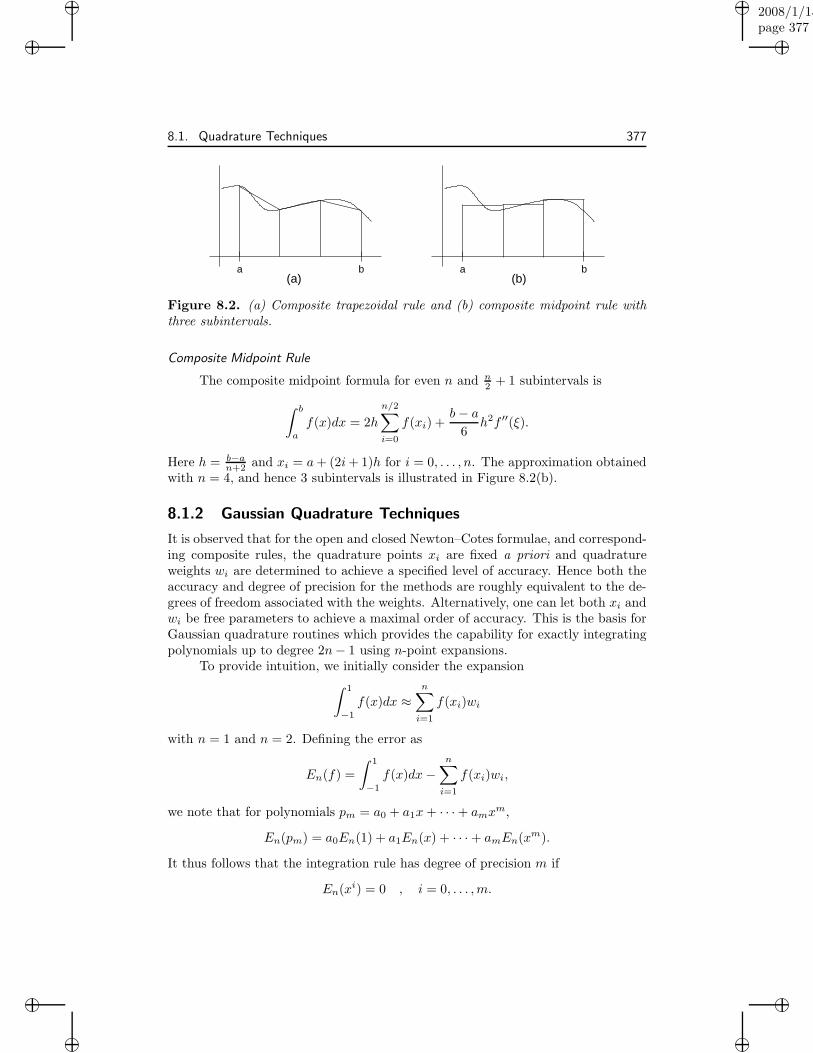
This mapping can also be used to construct composite Gaussian quadratureroutines and formulae appropriate for finite element and spline meshes. To illus-trate, consider the partition of [a, b] given by xj = a + jh, h = b−a
n , for j = 0, . . . , nas illustrated in Figure 8.3. The nodes and weights for the 4-point Gauss–Legendrerule on the subinterval [xj−1, xj ] are then
x1 = xj−1 + h
[12 −
√15+2
√30
2√
35
], w1 = 49h
12(18+√
30)
x2 = xj−1 + h
[12 −
√15−2
√30
2√
35
], w2 = 49h
12(18−√
30)
x3 = xj−1 + h
[12 +
√15−2
√30
2√
35
], w3 = 49h
12(18−√
30)
x4 = xj−1 + h
[12 +
√15+2
√30
2√
35
], w4 = 49h
12(18+√
30).
(8.12)
We note that this will integrate exactly piecewise polynomials of order up to 7.
x jx j−1 baxx x x
Figure 8.3. Partition of [a, b] into n subintervals and position of quadrature pointsfor the 4-point Gauss–Legendre rule on [xj−1, xj ].
8.1.3 2-D Quadrature Formulae
Approximation of weak formulations for plate and shell models requires the numer-ical evaluation of double integrals using quadrature rules of the form
∫ b
a
∫ d
c
f(x, y)dydx ≈nx∑
i=1
ny∑
j=1
f(xi, yj)wiwj .
Through the change of variables
∫ b
a
∫ d
c
f(x, y)dydx
=
(b − a
2
)(d − c
2
)∫ 1
−1
∫ 1
−1
f
(a + b + ξ(b − a)
2,c + d + υ(d − c)
2
)dυdξ,

“book”2008/1/15page 382
i
i
i
i
i
i
i
i
382 Chapter 8. Numerical Techniques
these integrals can be mapped to the rectangular domain [−1, 1] × [−1, 1] so weconsider first this case. This also provides the framework necessary for numericalintegration using rectangular elements. Finally, we summarize formulae for trian-gular elements as required for general finite element analysis.
Rectangular Domains
The formulae for rectangular domains are obtained by tensoring 1-D relations.For Gaussian formulae, this yields the nodal placement depicted in Figure 8.4.
4-Point Gauss–Legendre Quadrature
The tensor product of the 1-D formula (8.9) yields the 4-point quadraturerelation ∫ 1
−1
∫ 1
−1
f(ξ, υ)dυdξ ≈ f(a, a) + f(a, b) + f(b, a) + f(b, b)
where a = b = 1√3. This relation is exact for polynomials of degree 2. Hence this
algorithm would be employed when integrating linear quadrilateral elements.
9-Point Gauss–Legendre Quadrature
The tensor product of the 3-point formula from Table 8.1 yields
∫ 1
−1
∫ 1
−1
f(ξ, υ)dυdξ ≈ 25
81[f(a, a), f(a, c) + f(c, a) + f(c, c)]
+40
81[f(a, b) + f(c, b) + f(b, a) + f(b, c)] +
64
81f(b, b)
where a = −√
35 , b = 0 and c =
√35 . This relation is exact for degree 4 polynomials
so it would be used to integrate quadratic elements [390].
−1
−1 1
1
−1
−1 1
1
−1
−1 1
1
(b)(a) (c)
Figure 8.4. Quadrature points in a 2-D rectangular domain: (a) 1-point rule,(b) 4-point rule, and (c) 9-point rule.
Triangular Domains
For general finite element analysis, it is also necessary to consider quadra-ture formulae for triangular domains. This is often accomplished by consideringtransformations between physical space (x, y–coordinates) and computational space

“book”2008/1/15page 383
i
i
i
i
i
i
i
i
8.1. Quadrature Techniques 383
(0,1)υ
ξ(1,0)
(a)
T
y
x(b)
T~
Figure 8.5. (a) Master triangular element and (b) global element in physical space.
(ξ, υ–coordinates), as shown in Figure 8.5, so we summarize first the constructionof local coordinates that are independent of orientation.
The local coordinates L1, L2 and L3 are defined as the ratio between theperpendicular distance s to a side and the altitude h of the side as depicted inFigure 8.6(a). This implies that 0 ≤ Li ≤ 1. To elucidate a second property of theelements, consider the triangle T1, delineated by L1 as shown in Figure 8.6(b), andthe complete triangle T . From the area relations
AT1=
sb
2, AT =
hb
2,
it follows that L1 =AT1
AT. This motivates the designation of L1, L2, L3 as area
coordinates and establishes the relation
L1 + L2 + L3 = 1.
From the definition of the local coordinate L1, it follows that it satisfies theproperty
L1 =
1 at node i
0 at nodes i and k
with similar properties for L2 and L3. When combined with the linearity of the def-inition, this implies that local coordinates also provide the simplex linear elementsNi, Nj , Nk depicted in Figure 8.7; that is,
Ni = L1 , Nj = L2 , Nk = L3.
This proves crucial when defining quadrature properties for the finite element method.
T3
T2T1
L1L2
L3
(b)(a)
i
j
k
b
Figure 8.6. (a) Local coordinates L1, L2, L3 and (b) triangles T1, T2, T3 having theareas AT1
, AT2, AT3
.

“book”2008/1/15page 384
i
i
i
i
i
i
i
i
384 Chapter 8. Numerical Techniques
i NkNjN(1,0,0)
(0,1,0)
z
x
y
(0,0,1)
(1,0,0)
x
z
(0,1,0)y
(1,0,1)
x
(1,0,0)
z (0,1,1)
(0,1,0)y
Figure 8.7. Linear elements Ni, Nj and Nk.
Letting J denote the Jacobian for the transformation between physical andmaster triangular elements, it follows that
∫
T
f(x, y)dxdy =
∫
eT
f(L1, L2, L3) |J | dL1dL2
≈ 1
2
n∑
i=1
wif(L1i, L2i
, L3i)|Ji|.
The quadrature points, weights, and degrees of precision for n = 1, 2, 3 are summa-rized in Table 8.2 and higher-order formulae can be found in [205,462].
To illustrate, the 1-point quadrature relation∫
eT
f(ξ, υ)dξdυ ≈ 1
2f(1/3, 1/3)
integrates linear functions exactly whereas quadratic polynomials are integratedexactly by the formula
∫
eT
f(ξ, υ)dξdυ ≈ 1
6[f(1/2, 0) + f(0, 1/2) + f(1/2, 1/2)] .
Note that all of the formulae yield the triangle area A = 12 with f(ξ, υ) = 1.
n Degree of Local Coordinates Weights GeometricPrecision L1 L2 L3 w Location
1 1 13
13
13 1 a
a
3 2 12 0 1
213 a
12
12 0 1
3 b
0 12
12
13 c
4 3 13
13
13 − 27
48 a215
215
1115
2548 b
1115
215
215
2548 c
215
1115
215
2548 d
Table 8.2. Quadrature points and weights for triangular elements.
b
a c
a db
c

“book”2008/1/15page 385
i
i
i
i
i
i
i
i
8.2. Numerical Approximation of the Rod Model 385
8.2 Numerical Approximation of the Rod Model
In this section, we illustrate approximation techniques for the distributed rod modelsdeveloped in Section 7.3. For the general model (7.18), we first consider a directGalerkin discretization in space followed by a finite difference discretization in time.This yields global mass, stiffness and damping matrices, a semi-discrete systemappropriate for control design, and a fully discrete system feasible for simulations.Secondly, we consider an elemental analysis to demonstrate aspects of finite elementassembly often employed for 2-D and 3-D characterization.
8.2.1 Global Discretization in Space
Consider the weak model formulation (7.18),∫ ℓ
0
ρA∂2u
∂t2φdx +
∫ ℓ
0
[Y A
∂u
∂x+ cA
∂2u
∂x∂t
]dφ
dxdx =
∫ ℓ
0
fφdx
+A[a1P + a2P
2]∫ ℓ
0
dφ
dxdx −
[kℓu(t, ℓ) + cℓ
∂u
∂t(t, ℓ) + mℓ
∂2u
∂t2(t, ℓ)
]φ(ℓ),
(8.13)
where P = P − PR, which must hold for φ in the space of test functions
V =Φ = (φ, ϕ) ∈ L2(0, ℓ) × R |φ ∈ H1(0, ℓ), φ(0) = 0, φ(ℓ) = ϕ
.
The goal when constructing Galerkin solutions to (8.13) is to determine approximatesolutions in finite dimensional subspaces V N of V .
To construct V N , we consider a uniform partition of the interval [0, ℓ] withpoints xj = jh, j = 0, . . . , N and a uniform stepsize h = ℓ
N where N denotesthe number of subintervals. The spatial basis φjN
j=1 used to construct V N iscomprised of linear splines
φj(x) =1
h
x − xj−1 , xj−1 ≤ x < xj
xj+1 − x , xj ≤ x ≤ xj+1
0 , otherwise
, j = 1, . . . , N − 1
φN (x) =1
h
x − xN−1 , xN−1 ≤ x ≤ xN
0 , otherwise
(8.14)
as depicted in Figure 8.8. It is observed that the basis functions satisfy the essentialboundary condition φj(0) = 0 for j = 1, . . . , N . Furthermore, φjN
j=1 are differen-tiable throughout (0, ℓ), except at the countable set of gridpoints, and hence they
oj(x)
o (x)N
x x x xN−1 xNj−1 j j+1
Figure 8.8. Piecewise linear basis functions (a) φj(x) and (b) φN (x).

“book”2008/1/15page 386
i
i
i
i
i
i
i
i
386 Chapter 8. Numerical Techniques
are elements in H1(0, ℓ). Letting ϕj = φj(ℓ) and Φj = (φj , ϕj), the approximatingsubspace is defined to be
V N = span Φj .
The solution to (8.13) is approximated by the expansion
uN(t, x) =
N∑
j=1
uj(t)φj(x) (8.15)
which satisfies uN(t, 0) = 0 and can achieve arbitrary displacements at x = ℓ.A semi-discrete second-order matrix system is obtained by considering the
approximate solution uN(t, x) in (8.13) with the basis functions φiNi=1 employed
as test functions — this is equivalent to projecting the system (8.13) onto the finite-dimensional subspace V N . The interchange of integration and summation yields thesystem
N∑
j=1
uj(t)
∫ ℓ
0
ρAφiφjdx +
N∑
j=1
uj(t)
∫ ℓ
0
cAφ′iφ
′jdx +
N∑
j=1
uj(t)
∫ ℓ
0
Y Aφ′iφ
′jdx
=
∫ ℓ
0
fφidx + A[a1(P − PR) + a2(P − PR)2
] ∫ ℓ
0
φ′idx
−(kℓuN(t)φN (ℓ) + cℓuN(t)φN (ℓ) + mℓuN(t)φN (ℓ)
)φN (ℓ)
which holds for i = 1, . . . , N . This can be written as the second-order vector-valuedsystem
M u(t)+Q u+Ku(t) = f(t)+A[a1(P (E(t)) − PR) + a2(P (E(t)) − PR)2
]b (8.16)
whereu(t) = [u1(t), . . . , uN(t)]
T.
The global mass, stiffness and damping matrices have the components
[M ]ij =
∫ ℓ
0
ρAφiφj dx , i 6= N or j 6= N
∫ ℓ
0
ρAφiφj dx + mℓ , i = N and j = N
[K ]ij =
∫ ℓ
0
Y Aφ′iφ
′j dx , i 6= N or j 6= N
∫ ℓ
0
Y Aφ′iφ
′j dx + kℓ , i = N and j = N
[Q ]ij =
∫ ℓ
0
cAφ′iφ
′j dx , i 6= N or j 6= N
∫ ℓ
0
cAφ′iφ
′j dx + cℓ , i = N and j = N
(8.17)
“book”2008/1/15page 387
i
i
i
i
i
i
i
i
8.2. Numerical Approximation of the Rod Model 387
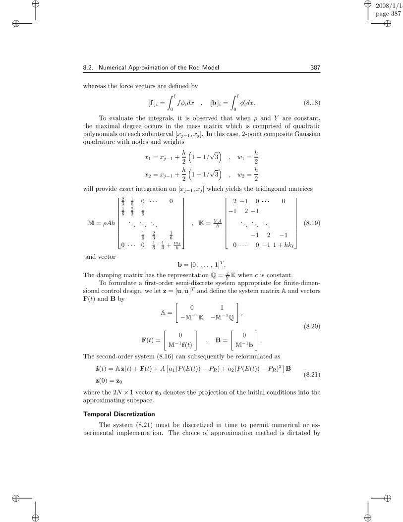
whereas the force vectors are defined by
[f ]i =
∫ ℓ
0
fφidx , [b ]i =
∫ ℓ
0
φ′idx. (8.18)
To evaluate the integrals, it is observed that when ρ and Y are constant,the maximal degree occurs in the mass matrix which is comprised of quadraticpolynomials on each subinterval [xj−1, xj ]. In this case, 2-point composite Gaussianquadrature with nodes and weights
x1 = xj−1 +h
2
(1 − 1/
√3)
, w1 =h
2
x2 = xj−1 +h
2
(1 + 1/
√3)
, w2 =h
2
will provide exact integration on [xj−1, xj ] which yields the tridiagonal matrices
M = ρAh
23
16 0 · · · 0
16
23
16
. . .. . .
. . .16
23
16
0 · · · 0 16
13 + mℓ
h
, K = Y Ah
2 −1 0 · · · 0
−1 2 −1
. . .. . .
. . .
−1 2 −1
0 · · · 0 −1 1 + hkℓ
(8.19)
and vectorb = [0 , . . . , 1]T .
The damping matrix has the representation Q = cY K when c is constant.
To formulate a first-order semi-discrete system appropriate for finite-dimen-sional control design, we let z = [u, u ]T and define the system matrix A and vectorsF(t) and B by
A =
[0 I
−M−1K −M−1Q
],
F(t) =
[0
M−1f(t)
], B =
[0
M−1b
].
(8.20)
The second-order system (8.16) can subsequently be reformulated as
z(t) = Az(t) + F(t) + A[a1(P (E(t)) − PR) + a2(P (E(t)) − PR)2
]B
z(0) = z0
(8.21)
where the 2N × 1 vector z0 denotes the projection of the initial conditions into theapproximating subspace.
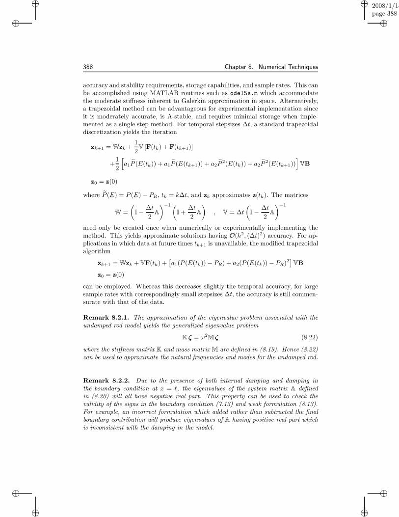
Temporal Discretization
The system (8.21) must be discretized in time to permit numerical or ex-perimental implementation. The choice of approximation method is dictated by
“book”2008/1/15page 388
i
i
i
i
i
i
i
i
388 Chapter 8. Numerical Techniques
accuracy and stability requirements, storage capabilities, and sample rates. This canbe accomplished using MATLAB routines such as ode15s.m which accommodatethe moderate stiffness inherent to Galerkin approximation in space. Alternatively,a trapezoidal method can be advantageous for experimental implementation sinceit is moderately accurate, is A-stable, and requires minimal storage when imple-mented as a single step method. For temporal stepsizes ∆t, a standard trapezoidaldiscretization yields the iteration
zk+1 = Wzk +1
2V [F(tk) + F(tk+1)]
+1
2
[a1P (E(tk)) + a1P (E(tk+1)) + a2P
2(E(tk)) + a2P2(E(tk+1))
]VB
z0 = z(0)
where P (E) = P (E) − PR, tk = k∆t, and zk approximates z(tk). The matrices
W =
(I − ∆t
2A
)−1(I +
∆t
2A
), V = ∆t
(I − ∆t
2A
)−1
need only be created once when numerically or experimentally implementing themethod. This yields approximate solutions having O(h2, (∆t)2) accuracy. For ap-plications in which data at future times tk+1 is unavailable, the modified trapezoidalalgorithm
zk+1 = Wzk + VF(tk) +[a1(P (E(tk)) − PR) + a2(P (E(tk)) − PR)2
]VB
z0 = z(0)
can be employed. Whereas this decreases slightly the temporal accuracy, for largesample rates with correspondingly small stepsizes ∆t, the accuracy is still commen-surate with that of the data.
Remark 8.2.1. The approximation of the eigenvalue problem associated with theundamped rod model yields the generalized eigenvalue problem
Kζ = ω2Mζ (8.22)
where the stiffness matrix K and mass matrix M are defined in (8.19). Hence (8.22)can be used to approximate the natural frequencies and modes for the undamped rod.
Remark 8.2.2. Due to the presence of both internal damping and damping inthe boundary condition at x = ℓ, the eigenvalues of the system matrix A definedin (8.20) will all have negative real part. This property can be used to check thevalidity of the signs in the boundary condition (7.13) and weak formulation (8.13).For example, an incorrect formulation which added rather than subtracted the finalboundary contribution will produce eigenvalues of A having positive real part whichis inconsistent with the damping in the model.

“book”2008/1/15page 389
i
i
i
i
i
i
i
i
8.2. Numerical Approximation of the Rod Model 389
8.2.2 Elemental Analysis
The spatial discretization technique detailed in Section 8.2.1 illustrates the gen-eral philosophy of Galerkin approximation including the definition of global basisfunctions and their use for defining an approximating subspace V N ⊂ V . In thissection, we summarize a local, elemental approach to the problem. Whereas the twotechniques yield equivalent mass, stiffness and damping matrices, the latter is sig-nificantly more efficient for general 2-D and 3-D geometries and hence is employedfor general finite element analysis of complex structures.
To simplify the discussion and facilitate energy analysis, we consider theregime employed in Section 7.3.2 and take c = f = P = mℓ = cℓ = kℓ = 0 inthe weak formulation (8.13). Additionally, we assume that ρ and Y are constant.This model quantifies the dynamics of an undamped and unforced rod that is fixedat x = 0 and free at x = ℓ. The space of test functions in this case is
V = H10 (0, ℓ) =
φ ∈ H1(0, ℓ) |φ(0) = 0
.
Local Basis Elements
To illustrate the construction of local mass and stiffness matrices, we initiallyconsider the approximation of rod dynamics on a local interval [0, h] as depicted inFigure 8.9(a). In accordance with the assumption that u is differentiable in x at allbut a countable number of points, we express displacements as
u(t, x) = a0(t) + a1(t)x
= ϕT (x)a(t)
where a(t) = [a0(t) , a1(t)]T and ϕ(x) = [1 , x]T . To formulate u in terms of the
nodal values uℓ(t) and ur(t) at x = 0 and x = ℓ, we note that[
uℓ(t)
ur(t)
]=
[1 0
1 h
][a0(t)
a1(t)
]
oru(t) = Ta(t)
where
T =
[1 0
1 h
], u(t) =
[uℓ(t)
ur(t)
].
1(x)o~
(x)o2~
ur (t)ul(t)
x=h(a) (b)
h
1
x=0
Figure 8.9. (a) Rod displacements uℓ(t) and ur(t) at the left and right endpoints
of the local interval [0, h]. (b) Local linear basis functions φ1(x) and φ2(x).

“book”2008/1/15page 390
i
i
i
i
i
i
i
i
390 Chapter 8. Numerical Techniques
By observing that a(t) = Su(t), where
S = T−1 =
[1 0
− 1h
1h
],
it follows that displacements can be represented as
u(t, x) = φT (x)u(t). (8.23)
Here φ(x) =[φ1(x), φ2(x)
]T
contains the local basis elements
φ1(x) = 1 − x
h, φ2(x) =
x
h
depicted in Figure 8.9(b).Note that (8.23) is a local version of the expansion (8.15) employed when
constructing approximate solutions using the global basis functions φjNj=1 defined
in (8.14). The local region [0, h] and global interval [xj−1, xj ] are analogous to themaster and physical triangles depicted in Figure 8.5 whereas the local basis setφ1, φ2 is the 1-D analogue of the 2-D elements Ni, Nj , Nk shown in Figure 8.7.
Hamiltonian Formulation
To specify a dynamic model quantifying the displacements u, we employ theHamiltonian framework detailed in Section 7.3.2 for the infinite dimensional prob-lem. Here we consider displacements u ∈ V N = spanφ1, φ2 as dictated by ourapproximation framework.
We first note that for this class of displacements, the squared strains andvelocities can be expressed as
u2x(t, x) = uT (t)ST D(x)Su(t)
u2t (t, x) = uT (t)ST F(x)Su(t)
where
D(x) = ϕx(x)ϕTx (x)T =
[0 0
0 1
], F(x) = ϕ(x)ϕT (x) =
[1 x
x x2
].
The potential and kinetic energies (7.20) can thus be expressed as
U =Y A
2uT (t)ST ·
∫ h
0
D(x)dx · Su(t)
K =ρA
2uT (t)ST ·
∫ h
0
F(x)dx · Su(t).
Application of Hamilton’s principle in the manner detailed in Section 7.3.2yields the relation
ρAST ·∫ h
0
F(x)dx · Su(t) + Y AST ·∫ h
0
D(x)dx · Su(t) = 0. (8.24)

“book”2008/1/15page 391
i
i
i
i
i
i
i
i
8.2. Numerical Approximation of the Rod Model 391
Local Mass and Stiffness Matrices
The weak formulation (8.24) can be written as
Meu(t) + Keu = 0
where
Me = ρAST ·∫ h
0
F(x)dx · S , Ke = Y AST ·∫ h
0
D(x)dx · S
are the local mass and stiffness matrices. Evaluation of the integrals yields theanalytic formulations
Me = ρAh
[13
16
16
13
], Ke = Y A
h
[1 −1
−1 1
].
Global Mass and Stiffness Matrices
To motivate the techniques used to construct global mass and stiffness ma-trices, we first partition the rod interval [0, ℓ] into two subregions as shown inFigure 8.10(a) — hence h = ℓ
2 . With the requirement that u1r(t) = u2ℓ(t), thenodal unknowns in this case are u(t) = [u1ℓ(t), u2ℓ(t), u2r(t)]
T . Combination of thelocal relations subsequently yields the global system
M u + Ku = 0
where the global mass and stiffness matrices are given by
M = ρAh
13
16 0
16
23
16
0 16
13
, K = Y A
h
1 −1 0
−1 2 −1
0 −1 1
.
We note that the second row in the mass matrix is obtained by summing the elementrelations
ρAℓ
2
(1
6u1ℓ +
1
3u2ℓ
)= 0
ρAℓ
2
(1
3u2ℓ +
1
6u2r
)= 0
after enforcing u1r = u2ℓ. A similar strategy is employed when constructing thestiffness matrix and the general procedure is illustrated in Figure 8.11(a).
xj−1 xj0 l 0 l
(b)(a)
Figure 8.10. Partition of the rod domain [0, ℓ] into (a) 2 subregions and (b) n sub-regions.

“book”2008/1/15page 392
i
i
i
i
i
i
i
i
392 Chapter 8. Numerical Techniques
(b)
(a)
Figure 8.11. Combination of elemental mass and stiffness matrices Me and Ke toconstruct global matrices M and K : (a) 2 subregions, and (b) n subregions.
The process for general partitions xj = jh, j = 0, 1, . . . , N with h = ℓN is
identical and leads to a similar summation process as shown in Figure 8.11(b).Enforcing the boundary condition u1ℓ = 0 subsequently yields the global mass andstiffness matrices
M = ρAh
23
16 0 · · · 0
16
23
16
. . .. . .
. . .16
23
16
0 · · · 0 16
13
, K = Y Ah
2 −1 0 · · · 0
−1 2 −1
. . .. . .
. . .
−1 2 −1
0 · · · 0 −1 1
. (8.25)
A comparison between (8.25) and (8.19) obtained through global analysis illustratesthat the matrices are identical when one takes mℓ = kℓ = 0 in the latter set.
The technique can be extended to incorporate linear and nonlinear inputsby employing the augmented action integral (7.25) and an extended Hamilton’sprinciple. Internal and boundary damping is incorporated by employing extendedconstitutive relations as detailed in the previous section.
Whereas the global discretization techniques and elemental analysis providethe same semi-discrete systems, the latter technique facilitates implementation forgeneral 2-D and 3-D geometries discretized using triangular meshes. Additionaldetails regarding finite element techniques for rod models can be found in [36,276].
8.2.3 Examples and Software
The performance of the discretized rod model is illustrated in Section 7.3.3 in thecontext of characterizing displacements generated by a stacked PZT actuator froman AFM stage. This example illustrates the effects of variable drive levels andthe incorporation of frequency-dependent hysteresis mechanisms via the nonlinearconstitutive relations developed in Chapter 2.
The performance of the approximation techniques when used to characterizethe hysteretic dynamics of a Terfenol-D transducer is reported in [119,120]. In thiscase, the domain wall model was used to provide the constitutive relations whichprovide the basis for constructing the distributed rod model. In both cases, themass, stiffness and damping matrices have the general representations (8.17) —

“book”2008/1/15page 393
i
i
i
i
i
i
i
i
8.3. Numerical Approximation of the Beam Model 393
M and K have the specific representations (8.19) when ρ and Y are constant — andthe input vectors are given by (8.18). The only differences in the models occur inthe scalar-valued input relations used to characterize the nonlinear hysteresis.
MATLAB m-files for implementing both the rod model and the model for thestacked PZT actuator employed in the AFM stage can be found at the websitehttp://www.siam.org/books/fr32.
8.3 Numerical Approximation of the Beam Model
The strategy for approximating the beam models developed in Section 7.4 is analo-gous to that employed for the rod models — spline or finite element discretizationsin space are used to construct semi-discrete systems appropriate for control designor subsequent temporal discretization for simulations. Unlike rod models, quan-tification of the bending moments or strain energy associated with bending yieldssecond derivatives in weak beam formulations which must be accommodated bybasis functions. In Section 8.3.1 we summarize the use of cubic B-splines to con-struct approximating subspaces whereas a cubic Hermite basis is constructed inSection 8.3.2 through techniques analogous to those of Section 8.2.2.
8.3.1 Cubic Spline Basis
We illustrate beam approximation in the context of a cantilever beam, having afixed-end at x = 0 and free-end at x = ℓ, with surface-mounted patches. For testfunctions φ in the space
V = H20 (0, ℓ) =
φ ∈ H2(0, ℓ) |φ(0) = φ′(0) = 0
,
the weak formulation of the model for linear inputs is∫ ℓ
0
ρ∂2w
∂t2φdx + γ
∫ ℓ
0
∂w
∂tφdx +
∫ ℓ
0
Y I∂2w
∂x2
d2φ
dx2dx
+
∫ ℓ
0
cI∂3w
∂x2∂t
d2φ
dx2dx =
∫ ℓ
0
fφdx + V (t)
∫ ℓ
0
kpd2φ
dx2dx
(8.26)
where the piecewise constants ρ, Y I, cI and kp are defined in (7.42) and (7.44).To formulate approximate solutions based on cubic B-Splines, consider the
partition xj = jh, where h = ℓN and j = 0, . . . , N . For j = −1, 0, 1, . . . , N + 1, it is
shown in [383] that standard cubic B-splines are defined by
φj(x) =1
h3
(x − xj−2)3 , x ∈ [xj−2, xj−1)
h3 + 3h2(x − xj−1) + 3h(x − xj−1)2 − 3(x − xj−1)
3 , x ∈ [xj−1, xj)
h3 + 3h2(xj+1 − x) + 3h(xj+1 − x)2 − 3(xj+1 − x)3 , x ∈ [xj , xj+1)
(xj+2 − x)3 , x ∈ [xj+1, xj+2)
0 , otherwise(8.27)
“book”2008/1/15page 394
i
i
i
i
i
i
i
i
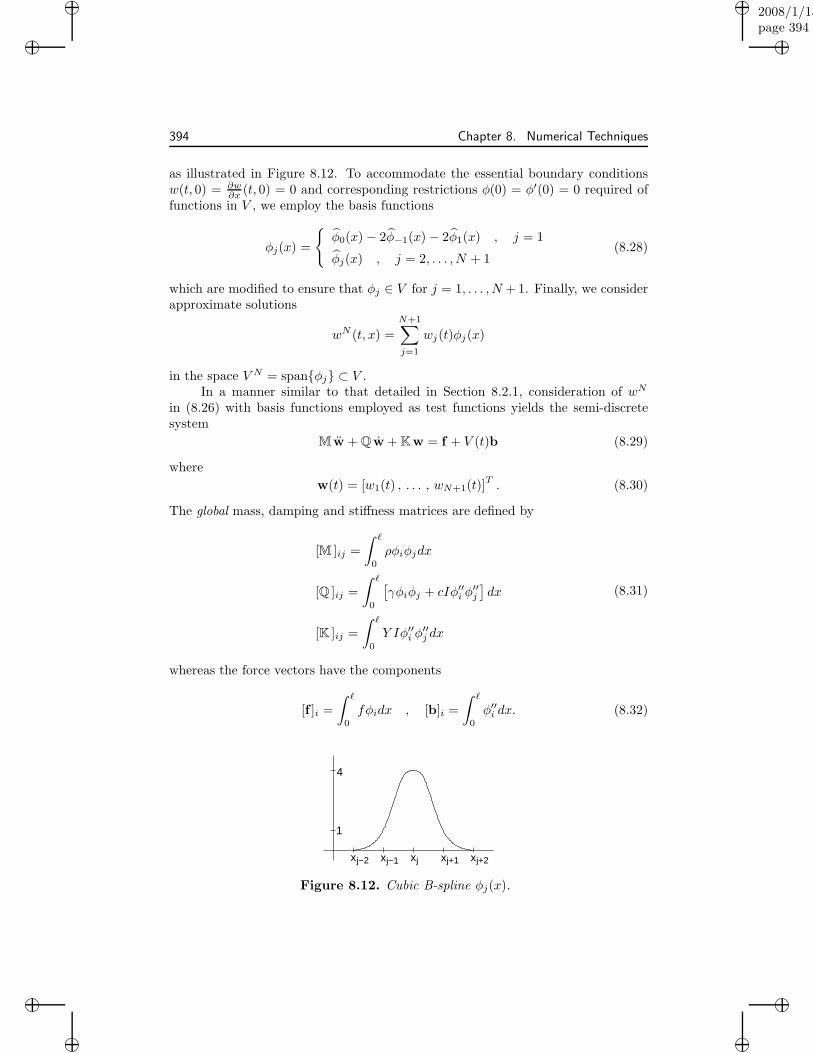
394 Chapter 8. Numerical Techniques
as illustrated in Figure 8.12. To accommodate the essential boundary conditionsw(t, 0) = ∂w
∂x (t, 0) = 0 and corresponding restrictions φ(0) = φ′(0) = 0 required offunctions in V , we employ the basis functions
φj(x) =
φ0(x) − 2φ−1(x) − 2φ1(x) , j = 1
φj(x) , j = 2, . . . , N + 1(8.28)
which are modified to ensure that φj ∈ V for j = 1, . . . , N + 1. Finally, we considerapproximate solutions
wN (t, x) =
N+1∑
j=1
wj(t)φj(x)
in the space V N = spanφj ⊂ V .In a manner similar to that detailed in Section 8.2.1, consideration of wN
in (8.26) with basis functions employed as test functions yields the semi-discretesystem
M w + Q w + Kw = f + V (t)b (8.29)
where
w(t) = [w1(t) , . . . , wN+1(t)]T . (8.30)
The global mass, damping and stiffness matrices are defined by
[M ]ij =
∫ ℓ
0
ρφiφjdx
[Q ]ij =
∫ ℓ
0
[γφiφj + cIφ′′
i φ′′j
]dx
[K ]ij =
∫ ℓ
0
Y Iφ′′i φ′′
j dx
(8.31)
whereas the force vectors have the components
[f ]i =
∫ ℓ
0
fφidx , [b]i =
∫ ℓ
0
φ′′i dx. (8.32)
xjxj−1xj−2 xj+2xj+1
1
4
Figure 8.12. Cubic B-spline φj(x).
“book”2008/1/15page 395
i
i
i
i
i
i
i
i
8.3. Numerical Approximation of the Beam Model 395
The second-order vector-value system (8.29) has the same form as (8.16) whichwas developed for the rod model and the techniques of Section 8.2.1 can be used toconstruct a first-order system appropriate for design and control.
Properties of Cubic Spline Approximates
We summarize here properties of the cubic spline approximates — additionalcomparison between this class of approximate solutions and the cubic Hermite ap-proximates developed in Section 8.3.2 can be found in Section 8.3.3.
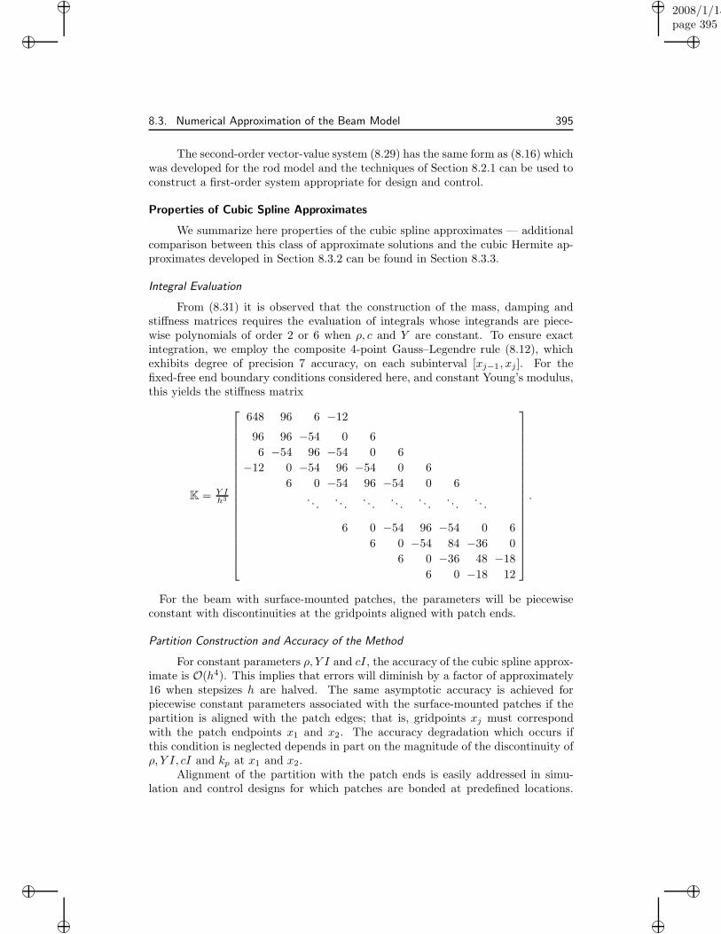
Integral Evaluation
From (8.31) it is observed that the construction of the mass, damping andstiffness matrices requires the evaluation of integrals whose integrands are piece-wise polynomials of order 2 or 6 when ρ, c and Y are constant. To ensure exactintegration, we employ the composite 4-point Gauss–Legendre rule (8.12), whichexhibits degree of precision 7 accuracy, on each subinterval [xj−1, xj ]. For thefixed-free end boundary conditions considered here, and constant Young’s modulus,this yields the stiffness matrix
K = Y Ih3
648 96 6 −12
96 96 −54 0 6
6 −54 96 −54 0 6
−12 0 −54 96 −54 0 6
6 0 −54 96 −54 0 6. . .
. . .. . .
. . .. . .
. . .. . .
6 0 −54 96 −54 0 6
6 0 −54 84 −36 0
6 0 −36 48 −18
6 0 −18 12
.
For the beam with surface-mounted patches, the parameters will be piecewiseconstant with discontinuities at the gridpoints aligned with patch ends.
Partition Construction and Accuracy of the Method
For constant parameters ρ, Y I and cI, the accuracy of the cubic spline approx-imate is O(h4). This implies that errors will diminish by a factor of approximately16 when stepsizes h are halved. The same asymptotic accuracy is achieved forpiecewise constant parameters associated with the surface-mounted patches if thepartition is aligned with the patch edges; that is, gridpoints xj must correspondwith the patch endpoints x1 and x2. The accuracy degradation which occurs ifthis condition is neglected depends in part on the magnitude of the discontinuity ofρ, Y I, cI and kp at x1 and x2.
Alignment of the partition with the patch ends is easily addressed in simu-lation and control designs for which patches are bonded at predefined locations.

“book”2008/1/15page 396
i
i
i
i
i
i
i
i
396 Chapter 8. Numerical Techniques
A more pertinent issue arises when addressing the problem of optimal patch loca-tion for which x1 and x2 are parameters determined through an optimization rou-tine [132, 155, 202]. This necessitates consideration of variable or adaptive meshesand constitutes an active research area.
Projection Method
It is important to note that approximation using the modified B-spline basis(8.28) constitutes a projection rather than interpolation method as is the case for thecubic Hermite methods summarized in Section 8.3.2. Hence the coefficients (8.30)do not approximate nodal values of the true solution and modified basis functionsare required to accommodate essential boundary conditions. In this sense, B-splineapproximation shares a projective kinship with globally defined spectral methods— e.g., Legendre or Fourier — while retaining the sparsity associated with locallydefined polynomial elements. As will be detailed in Section 8.3.3, the advantage ofcubic B-splines over cubic Hermite elements lies in the fact that half as many coef-ficients are required in the former case. The non-interpolatory nature of B-splinesconstitutes the primary disadvantage which is especially pertinent when accommo-dating boundary or interface conditions between components of the structure —e.g., curved and flat portions of THUNDER transducers.
8.3.2 Cubic Hermite Basis
To illustrate the construction of a finite element basis which interpolates displace-ments and slopes at the partition points, we initially consider the model (8.26) in theabsence of internal or air damping and external forces — hence c = γ = f = V = 0.Additionally, we take ρ and Y to be constant to highlight the structure of con-stituent matrices.
Local Mass and Stiffness Matrices
It was detailed in Section 7.4 that thin beam models quantify both the trans-verse displacement and rotation of the neutral line so we begin the elemental analysisby quantifying the displacements wℓ, wr and slopes θℓ, θr on an arbitrary interval[0, h] as depicted in Figure 8.13. Once we have constructed local mass and stiffnessmatrices, we will extend the analysis to partitions of the full beam interval [0, ℓ] toconstruct global system matrices.
wl
θl
θr
wr
x=0 x=h
Figure 8.13. Displacements wℓ, wr and slopes θℓ, θr at the ends of a cubic elementon the interval [0, h].

“book”2008/1/15page 397
i
i
i
i
i
i
i
i
8.3. Numerical Approximation of the Beam Model 397
Because the characterization of w(t) = [wℓ(t), θℓ(t), wr(t), θr(t)]T involves 4
degrees of freedom , we consider cubic representations
w(t, x) = a0(t) + a1(t)x + a2(t)x2 + a3(t)x
3
= ϕT (x)a(t)(8.33)
where a(t) = [a0(t), a1(t), a2(t), a3(t)]T and ϕ(x) = [1, x, x2, x3]T . By noting that
θ(t, x) = ∂w∂x (t, x) and enforcing the interpolation conditions at x = 0 and h, the
nodal coefficients can be represented as
w(t) = Ta(t)
where
T =
1 0 0 0
0 1 0 0
1 h h2 h3
0 1 2h 3h2
.
Substitution of a(t) = T−1w(t) into (8.33) yields the expansion
w(t, x) = φ T (x)w(t)
where φ = [φ1, φ2, φ3, φ4]T comprises the local cubic Hermite basis functions
φ1(x) =1
h3(h − x)2[2x + h] , φ3(x) =
1
h3x2[2(h − x) + h]
φ2(x) =1
h2x(x − h)2 , φ4(x) =
1
h2x2(x − h).
(8.34)
As shown in Figure 8.14, the elements φj(x) have displacement or slope values of 0or 1 at x = 0, h. This ensures that the coefficients w(t) = [wℓ(t), θℓ(t), wr(t), θr(t)]
T
interpolate the beam displacements and slopes at x = 0, h.From the relations
U =1
2Y I
∫ h
0
(∂2w
∂x2
)2
dx , K =1
2ρ
∫ h
0
(∂2w
∂t2
)2
dx
o4(x)~
h
h
1
1
h
h
o3(x)
1(x) (x)o2o~
~
~
Figure 8.14. Cubic Hermite basis functions φ1, . . . , φ4.

“book”2008/1/15page 398
i
i
i
i
i
i
i
i
398 Chapter 8. Numerical Techniques
for the potential energy due to bending and kinetic energy, it follows that for theclass of approximate displacements (8.33),
U =Y I
2wT (t)ST ·
∫ h
0
D(x)dx · Sw(t)
K =ρ
2wT (t)ST ·
∫ h
0
F(x)dx · Sw(t)
where S = T−1 and
D(x) = ϕxx(x)ϕxxT (x) =
0 0 0 0
0 0 0 0
0 0 4 12x
0 0 12x 36x2
F(x) = ϕ(x)ϕT (x) =
1 x x2 x3
x x2 x3 x5
x2 x3 x4 x5
x3 x4 x5 x6
.
Application of Hamilton’s principle in the manner detailed in Section 7.3.2yields the second-order vector system
Mew + Kew = 0
where the local mass and stiffness matrices are
Me =ρh
420
156 22h 54 −13h
22h 4h2 13h −3h2
54 13h 156 −22h
−13h −3h2 −22h 4h2
, Ke =
Y I
h3
12 6h −12 6h
6h 4h2 −6h 2h2
−12 −6h 12 −6h
6h 2h2 −6h 4h2
.
Global Mass and Stiffness Matrices
Global mass and stiffness matrices are constructed by combining local relationssubject to the constraint that displacements and slopes match at the interfaces. Toillustrate, we first subdivide the beam support [0, ℓ] into two subregions as depictedin Figure 8.10(a). By enforcing the interface conditions
w1r(t) = w2ℓ(t) , θ1r(t) = θ2ℓ(t),

“book”2008/1/15page 399
i
i
i
i
i
i
i
i
8.3. Numerical Approximation of the Beam Model 399
we obtain the global matrices
M =ρh
420
156 22h 54 −13h 0 0
22h 4h2 13h −3h2 0 0
54 13h 312 0 54 −13h
−13h −3h2 0 8h2 13h −3h2
0 0 54 13h 156 −22h
0 0 −13h −3h2 −22h 4h2
and
K =Y I
h3
12 6h −12 6h 0 0
6h 4h2 −6h 2h2 0 0
−12 −6h 24 0 −12 6h
6h 2h2 0 8h2 −6h 2h2
0 0 −12 −6h 12 −6h
0 0 6h 2h2 −6h 4h2
where h = ℓ2 .
Due to the fixed-end conditions at x = 0, it follows that w1ℓ = θ1ℓ = 0. Afterre-ordering the vector of nodal values as
w(t) = [w1r(t), w2r(t), θ1r(t), θ2r(t)]T
,
the dynamics are quantified by the system
Mw + Kw = 0
where
M = ρh420
312 54 0 −13h
54 156 13h −22h
0 13h 8h2 −3h2
−13h −22h −3h2 4h2
, K = Y I
h3
24 −12 0 6h
−12 12 −6h −6h
0 −6h 8h2 2h2
6h −6h 2h2 4h2
. (8.35)
The process for general partitions xj = jh with h = ℓN is analogous and leads
to a similar summation process when constructing global system matrices — seeFigure 8.15. As detailed in previous sections, internal damping can be incorporatedby employing more general constitutive relations based on the assumption thatstress is proportional to a linear combination of strain and strain rate.
Global Discretization
We illustrated in Section 8.2 that either global Galerkin techniques or lo-cal elemental analysis could be employed when implementing linear finite elementmethods. The same is true with cubic Hermite elements. Whereas the local ele-mental analysis illustrates the implementation philosophy for general 2-D and 3-D

“book”2008/1/15page 400
i
i
i
i
i
i
i
i
400 Chapter 8. Numerical Techniques
Figure 8.15. Combination of elemental mass and stiffness matrices Me and Ke toconstruct global matrices M and K.
structures, global Galerkin techniques analogous to those in Section 8.2 can bemore efficient to implement for beam discretization. The global discretization alsodemonstrates similarities and differences between the interpolatory cubic Hermiteapproximates and the projective cubic spline technique discussed in Section 8.3.1.
For the partition xj = jh, h = ℓN , j = 0, . . . , N , the global Hermite basis
functions are taken to be
φwj(x) =
1
h3
(x − xj−1)2[2(xj − x) + h] , x ∈ [xj−1, xj ]
(xj+1 − x)2[2(x − xj) + h] , x ∈ (xj , xj+1]
0 , otherwise
φθj(x) =
1
h2
(x − xj−1)2(x − xj) , x ∈ [xj−1, xj ]
(xj+1 − x)2(x − xj) , x ∈ (xj , xj+1]
0 , otherwise
for j = 1, . . . , N−1. The definitions of φwNand φθN
are analogous but involves onlythe interval [xN−1, xN ]. As illustrated in Figure 8.16, the global basis functions φwj
and φθjare the concatenation of the local displacement elements φ3, φ1 and slope
elements φ4, φ2 defined in (8.34) and shown in Figure 8.12.The approximating subspace is taken to be
V N = spanφwj
, φθj
N
j=1
and the approximate solution is
wN (t, x) =
N∑
j=1
wj(t)φwj(x) +
N∑
j=1
θj(t)φθj(x). (8.36)
We note that by omitting φw0and φθ0
, elements v ∈ V N are guaranteed to satisfyv(0) = v′(0) = 0 which ensures that V N ⊂ V = H2
0 (0, ℓ). The ordering of nodal co-efficients provided by (8.36) yields banded, tridiagonal mass, damping and stiffnessmatrices that are Toeplitz along all but the last row and column.

“book”2008/1/15page 401
i
i
i
i
i
i
i
i
8.3. Numerical Approximation of the Beam Model 401
xj−1 xj xj+1
xjxj−1 xj+1
oθjowj
1
Figure 8.16. Global Hermite basis functions φwjand φθj
.
The projection of (8.26) onto V N and use of basis functions as test functionsyields the second-order system
M w + Q w + Kw = f + V (t)b
where the 2N × 1 vector w(t) has the nodal ordering
w(t) = [w1(t), . . . , wN (t), θ1(t), . . . , θN (t)]T .
The global system matrices M, Q, K and vectors f ,b have definitions analogous to(8.31) and (8.32) where φi and φj now represent the combined basis φwi
, φθi
and φwj, φθj
. As with the matrices arising from the cubic B-spline discretizationdiscussed in Section 8.3.1, the integrals involve piecewise polynomials of degree lessthan or equal to 6 so exact integration is achieved using the composite 4-pointGauss–Legendre rule (8.12) on each subinterval [xj−1, xj ].
For constant stiffness Y I, this yields the stiffness matrix
K = Y Ih3
24 −12 0 6h
−12 24 −12 −6h 0 6h
. . .. . .
. . .. . .
. . .. . .
−12 24 −12 −6h 0 6h
12 12 −6h −6h
0 −6h 8h2 2h2
6h 0 −6h 2h2 8h2 2h2
. . .. . .
. . .. . .
. . .. . .
6h 0 −6h 2h2 8h2 2h2
6h −6h 2h2 4h2
. (8.37)
It is observed that the stiffness matrix K in (8.35), which was derived throughelemental analysis, is a special case of (8.37) when N = 2. For the beam withsurface-mounted patches, the differing values of Y I in the patch region are simplyincorporated in those regions of the partition which coincide with the patch. Themass and damping matrices are constructed in an analogous manner.
We note that the parameter ordering w(t) = [w1(t), θ1(t), . . . , wN (t), θN (t)]T
eliminates the block tridiagonal structure and yields block diagonal matrices where

“book”2008/1/15page 402
i
i
i
i
i
i
i
i
402 Chapter 8. Numerical Techniques
each block has a support of 6 diagonals. The disadvantage of this ordering scheme isthat the Toeplitz nature of the matrices is destroyed which complicates matrix con-struction. Additional details regarding elemental and global approximation usingcubic Hermite elements can be found in [36, 203,422].
8.3.3 Comparison between Cubic Spline and Cubic Hermite
Approximates
The cubic B-spline and cubic Hermite techniques detailed in Sections 8.3.1 and 8.3.2illustrate two commonly employed Galerkin techniques for approximating beammodels. Both provide O(h4) spatial convergence rates as long as partitions arealigned with patches to accommodate discontinuities in mass, damping, stiffnessand input parameters. As noted in Section 8.3.1, the cubic spline discretization is aprojection method whereas the cubic Hermite method is interpolatory in the sensethat the coefficients w(t) are nodal values of the displacement and slope at thepartition points. Hence the cubic spline technique is more closely related to generalGalerkin expansions — e.g., employing Legendre or Fourier bases — whereas thecubic Hermite expansion employs the finite element philosophy which, as detailedon pages 417–419 of Appendix A, is subsumed in the Galerkin framework.
The primary advantage of the cubic Hermite method lies in its interpolatorynature. This simplifies the enforcement of essential boundary conditions and facil-itates characterization of complex structures which require nodal matching at thejunction of differing geometries. For example, the transition from flat tabs to thecurved patch region in THUNDER transducers — see the models (7.103), (7.106),or (7.107) in Section 7.9 — is easily accommodated by matching nodal values withHermite elements whereas it is difficult to implement with cubic splines.
The disadvantage of the Hermite approximate is that it requires roughly twiceas many coefficients as the spline expansion since both displacements and slopesare discretized. The increased dimensionality of system matrices must be accom-modated when employing the model for control designs which require real-timeimplementation.
8.3.4 Examples and Software
Attributes of the discretized beam model, when used to characterize the PVDF–polyimide unimorph depicted in Figure 7.13, are illustrated in Section 7.4.1. Ex-perimental validation of the discretized model for a beam with surface-mountedpiezoceramic patches is addressed in Chapter 5 of [33].
MATLAB m-files for implementing the unimorph and beam models are locatedat the website http://www.siam.org/books/fr32.
8.4 Numerical Approximation of the Plate Model
In this section, we summarize approximation techniques for the rectangular andcircular plate models developed in Section 7.5. We consider regimes in which trans-verse and longitudinal displacements can be decoupled and focus on approximating

“book”2008/1/15page 403
i
i
i
i
i
i
i
i
8.4. Numerical Approximation of the Plate Model 403
the former using Galerkin expansions employing spline or Fourier bases in space. Asillustrated in Section 8.5 when discussing thin shell approximation, linear elementscan be employed to discretize longitudinal displacements if warranted by the appli-cation. A full discussion regarding finite element methods for plates is beyond thescope of this discussion and the reader is referred to [276, 390, 422, 527] for detailsabout this topic.
8.4.1 Rectangular Plate Approximation
We consider a rectangular plate with x ∈ [0, ℓ] and y ∈ [0, a] as depicted in Fig-ure 7.17. As in Section 7.5.1, we assume that the plate has thickness h and hasNA surface-mounted piezoceramic patches of thickness hI whose edges are parallelwith the x and y-axes. The plate is assumed to have fixed-edge conditions at x = 0,y = 0 and free boundary conditions for the remaining two edges. To simplify no-tation, we let Ω = [0, ℓ] × [0, a] denote the plate region. Finally, we consider linearinput regimes with voltages Vi(t) = V1i(t) = −V2i(t). Extension to nonlinear in-put regimes follows immediately when voltage inputs are replaced by the nonlinearpolarization relations.
From (7.65), the transverse displacements are quantified by the weak modelformulation
∫
Ω
ρ∂2w
∂t2φ − Mx
∂2φ
∂x2− 2Mxy
∂2φ
∂x∂y− My
∂2φ
∂y2− fnφ
dω = 0 (8.38)
for φ in the space of test functions
V = H20 (Ω) =
φ ∈ H2(Ω) |φ(0, y) = φx(0, y) = 0 for 0 ≤ y ≤ a,
φ(x, 0) = φy(x, 0) = 0 for 0 ≤ x ≤ ℓ.
The density ρ is specified by (7.48) and the moments are defined in (7.57) withcomponents specified in (7.58)–(7.63). We consider the case of linear patch inputsbut note that nonlinear inputs are accommodated in an identical manner.
The philosophy when approximating the dynamics of (8.38) is identical tothat employed in Sections 8.2 and 8.3 for the rod and beam models. The relation isprojected onto a spline-based finite-dimensional subspace V N ⊂ V to obtain a semi-discrete system appropriate for finite-dimensional control design. This vector-valuedsystem can subsequently be simulated by employing finite difference discretizationsin time or standard software for moderately stiff systems.
Consider a partition (xm, yn) of Ω where xm = mhx, yn = nhy, with hx =ℓ
Nx, hy = a
Nyand m = 0, . . . , Nx, n = 0, . . . , Ny. Using the definition (8.28), we
define modified cubic spline basis functions φm(x) and φn(y) on the intervals [0, ℓ]and [0, a]. The product space basis is then taken to be
Φk(x, y) = φm(x)φn(y) (8.39)
and the approximating subspace is
V N = span ΦkNw
k=1

“book”2008/1/15page 404
i
i
i
i
i
i
i
i
404 Chapter 8. Numerical Techniques
where Nw = (Nx +1)(Ny +1). Approximate displacements have the representation
wN (t, x, y) =
Nw∑
k=1
wk(t)Φk(x, y)
=
Nx+1∑
m=1
Ny+1∑
n=1
wmn(t)φm(x)φn(y).
The restriction of the infinite-dimensional model (8.38) to the finite-dimensionalsubspace V N ⊂ V yields the vector-valued system
M w + Q w + Kw = f +2YAd31c2
hA(1 − νA)
NA∑
i=1
Vi(t)bi (8.40)
where w(t) = [w1(t), . . . , wNw(t)]T . The mass and stiffness matrices are defined
componentwise by
[M ]jk =
∫
Ω
ρΦjΦkdω
[K ]jk = [K1]jk + [K2]jk + [K3]jk + [K4]jk + [K5]jk
where
[K1]jk =
∫
Ω
(YIh
3I
12(1 − ν2I )
+2YAc3
1 − ν2A
NA∑
i=1
χpei(x, y)
)∂2Φj
∂x2
∂2Φk
∂x2dω
[K2]jk =
∫
Ω
(YIh
3IνI
12(1 − ν2I )
+2YAc3νA
1 − ν2A
NA∑
i=1
χpei(x, y)
)∂2Φj
∂x2
∂2Φk
∂y2dω
[K3]jk =
∫
Ω
(YIh
3I
12(1 − ν2I )
+2YAc3
1 − ν2A
NA∑
i=1
χpei(x, y)
)∂2Φj
∂y2
∂2Φk
∂y2dω
[K4]jk =
∫
Ω
(YIh
3IνI
12(1 − ν2I )
+2YAc3νA
1 − ν2A
NA∑
i=1
χpei(x, y)
)∂2Φj
∂y2
∂2Φk
∂x2dω
[K5]jk =
∫
Ω
(YIh
3I
12(1 + νI)+
YAc3
1 + νA
NA∑
i=1
χpei(x, y)
)∂2Φj
∂x∂y
∂2Φk
∂x∂ydω.
The damping matrix Q is constructed in a manner analogous to K. Finally, thevectors are defined by
[f ]j =
∫
Ω
fnΦjdω
[bi]j =
∫
Ω
χpei(x, y)
(∂2Φj
∂x2+
∂2Φj
∂y2
)dω.
“book”2008/1/15page 405
i
i
i
i
i
i
i
i
8.4. Numerical Approximation of the Plate Model 405
The second-order system (8.40) has the same form as (8.16) which was de-veloped for the rod in Section 8.2.1. Hence the techniques in that section can beused to construct a corresponding first-order system appropriate for control designor simulation.
8.4.2 Circular Plate Approximation
The circular plate model (7.71) with space of test functions (7.70) represents a set-ting in which the geometry and differential operator are not the tensor product of1-D components. When combined with the inherent periodicity in θ, this motivatesconsideration of basis elements comprised of cubic B-splines in r and Fourier com-ponents in θ. We provide here an outline of the approximate system constructionand refer the reader to [430] for details regarding this development.
The circumferential component of the basis is taken to be φm(θ) = eimθ wherem = −M, . . . , M . The form of the radial component is motivated by the analyticBessel behavior of the undamped plate that is devoid of patches. Let φm
n (r) denote
the nth cubic spline modified to satisfy φmn (a) =
dφmn (a)dr = 0 — e.g., see (8.28) —
along with the conditiondφm
n (0)dr = 0 which is required to ensure differentiability at
the origin.The plate basis is then taken to be
Φk(r, θ) = r| bm|φmn (r)eimθ
where
m =
0 , m = 0
1 , m 6= 0.
As detailed in [430], the inclusion of the weighting term r| bm| is motivated by theasymptotic behavior of the Bessel functions as r → 0 and ensures the uniqueness ofthe solution at the origin. The approximating subspace is
V N = spanΦkand approximate solutions have the representation
wN (t, r, θ) =
Nw∑
k=1
wk(t)Φk(r, θ)
=
M∑
m=−M
Nm∑
n=1
wmn(t)r| bm|φmn (r)eimθ .
Here
Nm =
N , m = 0
N + 1 , m 6= 0.
where N denotes the number of modified cubic splines.Details regarding the construction of component matrices and vectors are pro-
vided in [430]. The performance of the discretized model when characterizing thedynamics of a circular plate is summarized in Section 7.5 and detailed in [430].
“book”2008/1/15page 406
i
i
i
i
i
i
i
i
406 Chapter 8. Numerical Techniques
8.4.3 Examples and Software
The accuracy and limitations of the discretized circular plate model for charac-terizing both axisymmetric and nonaxisymmetric plate vibrations are illustratedin Section 7.5.2. In the axisymmetric case, the model accurately quantifies lowto moderate frequency dynamics but overdamps high frequency modes which ischaracteristic of the Kelvin–Voigt damping model. It is illustrated that in the non-axisymmetric regime, which is truly 2-D, the model accurately characterizes thedynamics associated with 8 of the 11 measured modes.
The reader can obtain MATLAB m-files for the approximation of the rectan-gular plate model at the website http://www.siam.org/books/fr32.
8.5 Numerical Approximation of the Shell Model
The final structure under consideration is the cylindrical shell model (7.92) devel-oped in Section 7.7. To simplify the discussion, we consider fixed-edge conditionsu = v = w = ∂w
∂x = 0 at x = 0, ℓ and hence the space of test functions is
V = H10 (Ω) × H1
0 (Ω) × H20 (Ω)
where Ω = [0, ℓ] × [0, 2π] denotes the shell region and
H10 (Ω) =
φ ∈ H1(Ω) |φ(0, θ) = φ(ℓ, θ) = 0
H20 (Ω) =
φ ∈ H2(Ω) |φ(0, θ) = φ(ℓ, θ) = φx(0, θ) = φx(ℓ, θ) = 0
.
We summarize here the cubic spline–Fourier approximation method developedin [130] and illustrated for control design in [131]. As noted in the first citation, twophenomena which plague the approximation of shell models are shear locking andmembrane or shear-membrane locking. Shear locking, which has also been studiedextensively in the context of Reissner-Mindlin plate models, is due to element in-compatibility when enforcing the Kirchhoff-Love constraint of vanishing transverseshear strains as the shell thickness h tends to zero [14]. Membrane locking occurswhen the total deformation energy is bending-dominated and is due to smoothnessand asymptotic constraints in the shell model which are not appropriately repre-sented by the approximation method — e.g., [21, 22, 290, 380]. If these constraintsare not satisfied by approximating elements, the numerical solution is often overlystiff in the sense that the model exhibits bending dynamics which the approximatesolution cannot match. As detailed in [290], mesh sizes must be chosen significantlysmaller than the shell thickness to ensure accurate approximations with high-orderfinite elements in such bending-dominated regimes. It is noted that even with suchmesh size restrictions, low-order finite element methods often fail in such regimes.
The discussion in this section is meant to provide the reader with an overviewof issues associated with shell approximation and a brief summary of one discretiza-tion technique. Details and subtleties associated with this topic can found in [39,192]and previously cited references.

“book”2008/1/15page 407
i
i
i
i
i
i
i
i
8.5. Numerical Approximation of the Shell Model 407
Basis Construction and Approximating Subspaces
To approximate the longitudinal, circumferential and transverse displacementsu, v and w, it is necessary to construct bases for finite-dimensional subspaces ofH1
0 (Ω) and H20 (Ω). This is accomplished using linear and cubic splines modified to
accommodate the fixed boundary conditions.We consider a uniform partition along the x-axis with gridpoints xn = nh,
h = ℓN and n = 0, . . . , N . For n = 1, . . . , N − 1, we employ the linear splines
φun(x) = φvn
(x) =1
h
x − xn−1 , xn−1 ≤ x < xn
xn+1 − x , xn ≤ x ≤ xn+1
0 , otherwise
and modified cubic splines
φwn(x) =
φ0(x) − 2φ−1(x) − 2φ1(x) , n = 1
φn(x) , n = 2, . . . , N − 2
φN (x) − 2φN−1(x) − 2φN+1(x) , n = N − 1
where the standard B-splines are defined in (8.27). For n = 1, . . . , N − 1 andm = −M, . . . , M , the product space bases, in complex form, are taken to be
Φuk(θ, x) = eimθφun
(x)
Φvk(θ, x) = eimθφvn
(x)
Φwk(θ, x) = eimθφwn
(x).
To provide an equivalent real form, one can employ the representation
Φuk(θ, x) =
cos(mθ)1
sin(mθ)
φun
(x) , m = 1, . . . , M
with similar definitions for Φvkand Φwk
. The approximating subspaces are
V Nu = span Φuk
Nu
k=1
V Nv = span Φvk
Nv
k=1
V Nw = span Φwk
Nw
k=1
and the approximate displacements are represented by the expansions
uN (t, θ, x) =
Nu∑
k=1
uk(t)Φuk(θ, x)
vN (t, θ, x) =
Nv∑
k=1
vk(t)Φvk(θ, x)
wN (t, θ, x) =
Nw∑
k=1
wk(t)Φwk(θ, x).
(8.41)

“book”2008/1/15page 408
i
i
i
i
i
i
i
i
408 Chapter 8. Numerical Techniques
For a single partition, it follows that Nu = Nv = Nw = (2N −1)(2M +1). Throughthe construction of φun
, φvnand φwn
, the approximate displacements uN , vN andwN satisfy the fixed-end conditions and V N = V N
u × V Nv × V N
w ⊂ V . We note thatconsideration of real components yields the equivalent representation
uN (t, θ, x) =
N−1∑
n=1
u0n(t)φun(x)
+
M∑
m=1
N−1∑
n=1
umn(t) cos(mθ)φun(x) +
M∑
m=1
N−1∑
n=1
umn(t) sin(mθ)φun(x)
with similar expressions for vN (t, θ, x) and wN (t, θ, x).
System Matrices
To determine the generalized Fourier coefficients uk(t), vk(t) and wk(t), weemploy the same approach as in previous sections and orthogonalize the residualwith respect to the linearly independent test functions used to construct the approx-imating subspaces. To construct the resulting vector-valued system, we consolidatethe coefficients in the vectors
u(t) =
u1(t)...
uNu(t)
, v(t) =
v1(t)...
vNv(t)
, w(t) =
w1(t)...
wNw(t)
.
The full set of coefficients is then represented as ϑ(t) = [u(t),v(t),w(t)]T whereN = Nu + Nv + Nw.
The mass, stiffness and damping matrices have the form
M =
Um
Vm
Wm
,
K =
U11 + U12 V11 + V12 W11
U21 + U22 V21 + V22 W21
U31 V31
∑6k=1 W3k
,
Q =
U11 + U12 V11 + V12 W11
U21 + U22 V21 + V22 W21
U31 V31
∑6k=1 W3k
and the exogenous vectors are
f(t) = [fu , fv , fw]T , b = [bu , bv , , 0]T .

“book”2008/1/15page 409
i
i
i
i
i
i
i
i
8.5. Numerical Approximation of the Shell Model 409
The various submatrices contain individual components which arise when the weakformulation (7.92) is restricted to V N . For example, the approximation of the massand stiffness components in the longitudinal equation of (7.92) yields
[Um]jk =
∫
Ω
ρhRΦukΦuj
dω,
[U11]jk =
∫
Ω
Y hR
1 − ν2
∂Φuk
∂x
∂Φuj
∂xdω,
[V11]jk =
∫
Ω
Y hν
1 − ν2
∂Φvk
∂θ
∂Φuj
∂xdω,
[W11]jk =
∫
Ω
Y hν
1 − ν2Φwk
∂Φuj
∂xdω,
[V12]jk =
∫
Ω
Y h
2(1 + ν)
∂Φvk
∂x
∂Φuj
∂θdω,
[U12]jk =
∫
Ω
Y h
2R(1 + ν)
∂Φuk
∂θ
∂Φuj
∂θdω,
[fu]j =
∫
Ω
RfxΦujdω,
[bu]j =
∫
Ω
Rh
1 − ν
∂Φuj
∂xdω
with similar expressions for the remaining submatrices.In the usual manner, the second-order system
M ϑ(t) + Qϑ(t) + Kϑ(t) = f(t) +[a1(P (E(t)) − PR) + a2(P (E(t)) − PR)2
]b
ϑ(0) = ϑ0 , ϑ(0) = ϑ1
can be reformulated as the first-order Cauchy equation
zN (t) = Az(t) + F(t) +[a1(P (E(t)) − PR) + a2(P (E(t)) − PR)2
)B
z(0) = z0 ,
where z = [ϑ(t), ϑ(t)]T and
A =
[0 I
−M−1K −M−1Q
], F(t) =
[0
M−1(t)
], B =
[0
M−1b
].
The system in this form is anemable to simulation, parameter estimation and controldesign. Note that the system can be adapted to alternative boundary conditionsthrough modifications of the first and last basis functions. Flexibility in this regardis also a hallmark of the method.