CHAPTER 8. LIFE-CYCLE COST AND PAYBACK PERIOD …
52
CHAPTER 8. LIFE-CYCLE COST AND PAYBACK PERIOD ANALYSIS TABLE OF CONTENTS 8.1 INTRODUCTION ........................................................................................................... 8-1 8.1.1 General Approach for LCC and Payback Period Analysis .............................................. 8-1 8.1.2 Overview of LCC and Payback Period Inputs ................................................................. 8-2 8.2 LIFE-CYCLE COST INPUTS ........................................................................................ 8-6 8.2.1 Total Installed Cost Inputs ............................................................................................... 8-6 8.2.1.1 Baseline Manufacturer Cost ........................................................................... 8-8 8.2.1.2 Markups ......................................................................................................... 8-9 8.2.1.3 Overall Markup .............................................................................................. 8-9 8.2.1.4 Standard-Level Manufacturer Cost Increases .............................................. 8-10 8.2.1.5 Installation Cost ........................................................................................... 8-10 8.2.1.6 Total Installed Cost ...................................................................................... 8-11 8.2.1.7 Future Product Prices ................................................................................... 8-12 8.2.2 Operating Cost Inputs .................................................................................................... 8-14 8.2.2.1 Annual Energy and Water Consumption ..................................................... 8-16 8.2.2.2 Energy and Water Prices .............................................................................. 8-18 8.2.2.3 Energy and Water Price Trends ................................................................... 8-25 8.2.2.4 Repair and Maintenance Costs..................................................................... 8-27 8.2.3 Product Lifetime ............................................................................................................ 8-28 8.2.4 Discount Rates ............................................................................................................... 8-30 8.2.5 Effective Date of Standard ............................................................................................. 8-32 8.2.6 Equipment Assignment for the Base Case ..................................................................... 8-33 8.3 PAYBACK PERIOD INPUTS ...................................................................................... 8-34 8.4 LIFE-CYCLE COST AND PAYBACK PERIOD RESULTS ...................................... 8-35 8.4.1 Base Case LCC Distributions ........................................................................................ 8-35 8.4.2 Standard-Level Distributions of LCC Impacts .............................................................. 8-38 8.4.3 LCC and PBP Results .................................................................................................... 8-38 8.5 REBUTTABLE PAYBACK PERIOD .......................................................................... 8-44 8.5.1 Metric ............................................................................................................................. 8-44 8.5.2 Inputs.............................................................................................................................. 8-44 8.5.3 Results ............................................................................................................................ 8-45 LIST OF TABLES Table 8.1.1 LCC and PBP Input Summary ............................................................................. 8-5 Table 8.2.1 Inputs for Total Installed Cost ............................................................................. 8-7 Table 8.2.2 Commercial Clothes Washers: Baseline Manufacturer Costs ............................. 8-8 Table 8.2.3 Summary of Average Markups ............................................................................ 8-9 Table 8.2.4 Overall Markups ................................................................................................ 8-10 8-i
Transcript of CHAPTER 8. LIFE-CYCLE COST AND PAYBACK PERIOD …
CHAPTER 8. LIFE-CYCLE COST AND PAYBACK PERIOD ANALYSIS
TABLE OF CONTENTS 8.1 INTRODUCTION ........................................................................................................... 8-1 8.1.1 General Approach for LCC and Payback Period Analysis .............................................. 8-1 8.1.2 Overview of LCC and Payback Period Inputs ................................................................. 8-2 8.2 LIFE-CYCLE COST INPUTS ........................................................................................ 8-6 8.2.1 Total Installed Cost Inputs ............................................................................................... 8-6
8.2.1.1 Baseline Manufacturer Cost ........................................................................... 8-8 8.2.1.2 Markups ......................................................................................................... 8-9 8.2.1.3 Overall Markup .............................................................................................. 8-9 8.2.1.4 Standard-Level Manufacturer Cost Increases .............................................. 8-10 8.2.1.5 Installation Cost ........................................................................................... 8-10 8.2.1.6 Total Installed Cost ...................................................................................... 8-11 8.2.1.7 Future Product Prices ................................................................................... 8-12
8.2.2 Operating Cost Inputs .................................................................................................... 8-14 8.2.2.1 Annual Energy and Water Consumption ..................................................... 8-16 8.2.2.2 Energy and Water Prices .............................................................................. 8-18 8.2.2.3 Energy and Water Price Trends ................................................................... 8-25 8.2.2.4 Repair and Maintenance Costs ..................................................................... 8-27
8.2.3 Product Lifetime ............................................................................................................ 8-28 8.2.4 Discount Rates ............................................................................................................... 8-30 8.2.5 Effective Date of Standard ............................................................................................. 8-32 8.2.6 Equipment Assignment for the Base Case ..................................................................... 8-33 8.3 PAYBACK PERIOD INPUTS ...................................................................................... 8-34 8.4 LIFE-CYCLE COST AND PAYBACK PERIOD RESULTS ...................................... 8-35 8.4.1 Base Case LCC Distributions ........................................................................................ 8-35 8.4.2 Standard-Level Distributions of LCC Impacts .............................................................. 8-38 8.4.3 LCC and PBP Results .................................................................................................... 8-38 8.5 REBUTTABLE PAYBACK PERIOD .......................................................................... 8-44 8.5.1 Metric ............................................................................................................................. 8-44 8.5.2 Inputs.............................................................................................................................. 8-44 8.5.3 Results ............................................................................................................................ 8-45
LIST OF TABLES Table 8.1.1 LCC and PBP Input Summary ............................................................................. 8-5 Table 8.2.1 Inputs for Total Installed Cost ............................................................................. 8-7 Table 8.2.2 Commercial Clothes Washers: Baseline Manufacturer Costs ............................. 8-8 Table 8.2.3 Summary of Average Markups ............................................................................ 8-9 Table 8.2.4 Overall Markups ................................................................................................ 8-10
8-i

Table 8.2.5 Top-Loading Commercial Clothes Washers: Standard-Level Manufacturer Cost Increases .................................................................................................... 8-10
Table 8.2.6 Front-Loading Commercial Clothes Washers: Standard-Level Manufacturer Cost Increases.............................................................................. 8-10
Table 8.2.7 Commercial Clothes Washers: Baseline Installation Costs ............................... 8-11 Table 8.2.8 Top-Loading Commercial Clothes Washers: Consumer Equipment Prices,
Installation Costs, and Total Installed Costs ...................................................... 8-11 Table 8.2.9 Front-Loading Commercial Clothes Washers: Consumer Equipment
Prices, Installation Costs, and Total Installed Costs .......................................... 8-12 Table 8.2.10 Inputs for Operating Cost................................................................................... 8-15 Table 8.2.11 Top-Loading Commercial Clothes Washers, Multi-Family Application:
Annual Energy and Water Use by Efficiency Level .......................................... 8-17 Table 8.2.12 Top-Loading Commercial Clothes Washers, Laundromat Application:
Annual Energy and Water Use by Efficiency Level .......................................... 8-17 Table 8.2.13 Front-Loading Commercial Clothes Washers, Multi-Family Application:
Annual Energy and Water Use by Efficiency Level .......................................... 8-18 Table 8.2.14 Front-Loading Commercial Clothes Washers, Laundromat Application:
Annual Energy and Water Use by Efficiency Level .......................................... 8-18 Table 8.2.15 Average Commercial Electricity Prices in 2012 ................................................ 8-20 Table 8.2.16 Average Commercial Electricity Prices for Commercial Clothes Washers
in 2013 ............................................................................................................... 8-21 Table 8.2.17 Average Commercial Natural Gas Prices in 2012 ............................................. 8-23 Table 8.2.18 Average Per-Unit-Volume Water and Waste Water Prices in 2012 .................. 8-25 Table 8.2.19 Top-Loading Commercial Clothes Washer Annualized Repair Costs .............. 8-28 Table 8.2.20 Front-Loading Commercial Clothes Washer Annualized Repair Costs ............ 8-28 Table 8.2.21 Commercial Clothes Washers: Product Lifetime Estimates and Sources ........ 8-29 Table 8.2.22 Commercial Clothes Washers: Average, Minimum, and Maximum
Product Lifetimes ............................................................................................... 8-29 Table 8.2.23 Risk free rate and equity risk premium, 2004 – 2013 ........................................ 8-31 Table 8.2.24 Weighted Average Cost of Capital for Sectors that Purchase Washers ............. 8-32 Table 8.2.25 Top-Loading Commercial Clothes Washers: Base Case Market Shares ........... 8-33 Table 8.2.26 Front-Loading Commercial Clothes Washers: Base Case Market Shares......... 8-34 Table 8.4.1 Summary of LCC and PBP Results by Efficiency Level for Top-Loading
Commercial Clothes Washers, Multi-Family Application ................................ 8-39 Table 8.4.2 Summary of LCC and PBP Results by Efficiency Level for Top-Loading
Commercial Clothes Washers, Laundromat Application .................................. 8-39 Table 8.4.3 Summary of Life-Cycle Cost Savings Relative to the Base Case Efficiency
Distribution for Top-Loading Commercial Clothes Washers, Multi-Family Application ......................................................................................................... 8-39
Table 8.4.4 Summary of Life-Cycle Cost Savings Relative to the Base Case Efficiency Distribution for Top-Loading Commercial Clothes Washers, Laundromat Application ......................................................................................................... 8-40
Table 8.4.5 Summary of LCC and PBP Results by Efficiency Level for Front-Loading Commercial Clothes Washers, Multi-Family Application ................................ 8-40
8-ii

Table 8.4.6 Summary of LCC and PBP Results by Efficiency Level for Front-Loading Commercial Clothes Washers, Laundromat Application .................................. 8-40
Table 8.4.7 Summary of Life-Cycle Cost Savings Relative to the Base Case Efficiency Distribution for Front-Loading Commercial Clothes Washers, Multi-Family Application ............................................................................................ 8-41
Table 8.4.8 Summary of Life-Cycle Cost Savings Relative to the Base Case Efficiency Distribution for Front-Loading Commercial Clothes Washers, Laundromat Application ......................................................................................................... 8-41
Table 8.5.1 Top-Loading Commercial Clothes Washers, Multi-Family Application: Rebuttable Payback Periods ............................................................................... 8-45
Table 8.5.2 Top-Loading Commercial Clothes Washers, Laundromat Application: Rebuttable Payback Periods ............................................................................... 8-46
Table 8.5.3 Front-Loading Commercial Clothes Washers, Multi-Family Application: Rebuttable Payback Periods ............................................................................... 8-46
Table 8.5.4 Front-Loading Commercial Clothes Washers, Laundromat Application: Rebuttable Payback Periods ............................................................................... 8-46
LIST OF FIGURES
Figure 8.1.1 Flow Diagram of Inputs for the Determination of LCC and PBP ....................... 8-4 Figure 8.2.1 Historic Nominal and Deflated Producer Price Indexes for Commercial
Laundry and Drycleaning Machinery ................................................................ 8-13 Figure 8.2.2 Historic Nominal and Deflated Producer Price Indexes for Household
Laundry Equipment ........................................................................................... 8-14 Figure 8.2.3 Electricity Price Trends...................................................................................... 8-26 Figure 8.2.4 Natural Gas Price Trends ................................................................................... 8-26 Figure 8.2.5 Water Price Trend .............................................................................................. 8-27 Figure 8.4.1 Top-Loading Commercial Clothes Washers, Multi-Family Application:
Base Case LCC Distribution .............................................................................. 8-36 Figure 8.4.2 Top-Loading Commercial Clothes Washers, Laundromat Application:
Base Case LCC Distribution .............................................................................. 8-36 Figure 8.4.3 Front-Loading Commercial Clothes Washers, Multi-Family Application:
Base Case LCC Distribution .............................................................................. 8-37 Figure 8.4.4 Front-Loading Commercial Clothes Washers, Laundromat Application:
Base Case LCC Distribution .............................................................................. 8-37 Figure 8.4.5 Front-Loading Commercial Clothes Washers, Multi-Family Application:
Distribution of LCC Impacts for EL2 ................................................................ 8-38 Figure 8.4.6 Range of LCC Savings for Top-Loading Commercial Clothes Washers,
Multi-Family ...................................................................................................... 8-42 Figure 8.4.7 Range of LCC Savings for Top-Loading Commercial Clothes Washers,
Laundromat ........................................................................................................ 8-42 Figure 8.4.8 Range of LCC Savings for Front-Loading Commercial Clothes Washers,
Multi-Family ...................................................................................................... 8-43 Figure 8.4.9 Range of LCC Savings for Front-Loading Commercial Clothes Washers,
Laundromat ........................................................................................................ 8-43
8-iii

CHAPTER 8. LIFE-CYCLE COST AND PAYBACK PERIOD ANALYSIS
8.1 INTRODUCTION
This chapter describes the Department of Energy (DOE)’s methodology for analyzing the economic impacts of possible energy efficiency standards on individual consumers. The effect of standards on individual consumers includes a change in operating expense (usually decreased) and a change in purchase price (usually increased). This chapter describes three metrics DOE used in the consumer analysis to determine the effect of standards on individual consumers:
• Life-cycle cost (LCC) is the total consumer expense over the life of an appliance, including purchase expense and operating costs (including energy expenditures). DOE discounts future operating costs to the time of purchase, and sums them over the lifetime of the equipment.
• Payback period (PBP) measures the amount of time it takes customers to recover the
assumed higher purchase price of more energy-efficient equipment through lower operating costs.
• Rebuttable payback period is a special case of the PBP. Where LCC and PBP are
estimated over a range of inputs reflecting actual conditions, rebuttable payback period is based on laboratory conditions, specifically DOE test procedure inputs.
Inputs to the LCC and PBP are discussed in sections 8.2 and 8.3, respectively, of this chapter. Results for the LCC and PBP are presented in section 8.4. The rebuttable PBP is discussed in section 8.5. Key variables and calculations are presented for each metric. DOE performed the calculations discussed here using a series of Microsoft Excel® spreadsheets which are accessible on the Internet (http://www.eere.energy.gov/buildings/appliance_standards/). Details and instructions for using the spreadsheets are discussed in Appendix 8A.
8.1.1 General Approach for LCC and Payback Period Analysis
Recognizing that several inputs to the determination of consumer LCC are either variable or uncertain, DOE conducted the LCC analysis by modeling both the uncertainty and variability in the inputs using Monte Carlo simulation and probability distributions. A detailed explanation of Monte Carlo simulation and the use of probability distributions is contained in Appendix 8A. DOE developed LCC spreadsheet models incorporating both Monte Carlo simulation and probability distributions by using Microsoft Excel® spreadsheets combined with Crystal Ball® (a commercially available add-in program). As described in Chapter 7, DOE established the variability and uncertainty in energy and water use by defining the uncertainty and variability in the usage (in cycles per day) of the
8-1
equipment. As will be described later in this chapter, the variability and uncertainty in energy and water pricing are characterized by regional differences in energy and water prices. DOE displays the LCC results as distributions of impacts compared to the baseline conditions. Results are presented at the end of this chapter and are based on 10,000 samples per Monte Carlo simulation run. To illustrate the implications of the analysis, DOE generated a frequency chart depicting the variation in LCC for each standard level considered. The payback period is measured relative to the baseline product. The calculation uses average values for the inputs. It is calculated by dividing the change in installed cost by the change in first year operating cost for the baseline efficiency level and each increased efficiency level.
8.1.2 Overview of LCC and Payback Period Inputs
The LCC is the total consumer expense over the life of the equipment, including purchase expense and operating expense (including energy expenditures). DOE discounts future operating expenses to the time of purchase and sums them over the lifetime of the equipment. The PBP is the change in purchase expense due to an increased efficiency standard divided by the change in annual operating expense that results from the standard. It represents the number of years it will take the customer to recover the increased purchase expense through decreased operating expenses. DOE categorizes inputs to the LCC and PBP analysis as follows: (1) inputs for establishing the purchase expense, otherwise known as the total installed cost, and (2) inputs for calculating the operating cost. The primary inputs for establishing the total installed cost are:
• Baseline manufacturer cost: The costs incurred by the manufacturer to produce equipment meeting existing minimum efficiency standards.
• Standard-level manufacturer cost increases: The change in manufacturer cost associated
with producing equipment to meet a particular standard level. • Markups and sales tax: The markups and sales tax associated with converting the
manufacturer cost to a consumer equipment price. The markups and sale tax are described in detail in Chapter 7, Markups for Equipment Price Determination.
• Installation cost: The cost to the consumer of installing the equipment. The installation
cost represents all costs required to install the equipment other than the marked-up consumer equipment price. The installation cost includes labor, overhead, and any miscellaneous materials and parts. Thus, the total installed cost equals the consumer equipment price plus the installation cost.
8-2

The primary inputs for calculating the operating cost are:
• Equipment energy and water consumption: The equipment energy consumption is the site energy use associated with operating the equipment. The water consumption is the site water use associated with operating the equipment. Chapter 7, Energy and Water Use Analysis, details how DOE determined the equipment energy and water consumption based on various data sources. The per cycle energy and water use for the efficiency levels analyzed here are an input from the Engineering Analysis, as described in Chapter 5. Since the units selected for tests across efficiency levels varied in tub volume, DOE adjusted the annual number of cycles to maintain consistent loading across all tub volumes. To make this adjustment, DOE assumed that 50 percent of consumers fill tub to capacity instead of assuming that customers would self-select an appropriate sized washer in a laundromat.
• Equipment efficiency: The equipment efficiency dictates the equipment energy and water
consumption associated with standard-level equipment (i.e., equipment with efficiencies greater than baseline equipment). Chapter 7, Energy and Water Use Determination, details how energy and water consumption change with increasing equipment efficiency.
• Energy and water prices: Energy and water prices are the prices paid by consumers for
energy (i.e., electricity, gas, or oil) and water. DOE determined current energy prices based on data from the DOE- EIA. DOE determined water prices based on data from the American Water Works Association (AWWA).
• Energy and water price trends: DOE used the EIA Annual Energy Outlook
2014(AEO2014) to forecast energy prices into the future. For the results presented in this chapter, DOE used the AEO2014 reference case to forecast future energy prices. DOE used consumer price index data specific to water and sewerage maintenance from the Bureau of Labor Statistics as the basis for its water price trend.
• Repair and maintenance costs: Repair costs are associated with repairing or replacing
components that have failed. Maintenance costs are associated with maintaining the operation of the equipment.
• Lifetime: The age at which the equipment is retired from service.
• Discount rate: The rate at which DOE discounted future expenditures to establish their
present value. Figure 8.1.1 graphically depicts the relationships between the installed cost and operating cost inputs for the calculation of the LCC and PBP. In the figure below, the yellow boxes indicate the inputs, the green boxes indicate intermediate outputs, and the blue boxes indicate the final outputs (the LCC and PBP).
8-3

Figure 8.1.1 Flow Diagram of Inputs for the Determination of LCC and PBP Table 8.1.1 summarizes the input values that DOE used to calculate the LCC and PBP. Each table summarizes the total installed cost inputs and the operating cost inputs including the lifetime, discount rate, and energy and water price trends. DOE characterized all of the total cost inputs with single-point values, but characterized several of the operating cost inputs with probability distributions that capture the input’s uncertainty and/or variability. For those inputs characterized with probability distributions, the values provided in the following tables are the average or typical values. Also listed in the following tables is the section of the technical support document (TSD) where more detailed information on the inputs can be found.
Energy and Water Use
Energy and Water Prices
From Energy and Water Use
Analysis(Use is a
function of Efficiency)
Installation Cost
Equipment Price
From Engineering
Analysis(Price is a function of Efficiency)
From Markups Analysis
Baseline Manufacturer
Price
Std-Level Manufacturer
Price
Consumer Retail Price
Markup
Sales Tax
Repair Cost
Maintenance Cost
Annual Energy and Water Expense
Lifetime
Discount Rate
Energy and Water Price
Annual Operating Expense
Total Installed Cost
Lifetime Operating Expense
Payback Life-Cycle Cost
8-4

Table 8.1.1 LCC and PBP Input Summary
Input Product Class Average or Typical Value Characterization
TSD Section Reference
Total Installed Cost Inputs
Baseline Manufacturer Cost
Top-Loading 1.15 MEF/8.90 IWF = $532.40 Single-Point Value
8.2.1.2 Front-Loading 1.65 MEF/5.20 IWF = $844.23 Single-Point Value
Standard-Level Manufacturer Cost Increase
Top-Loading
1.35 MEF/8.80 IWF = $0.00 1.55 MEF/6.90 IWF = $39.63 Single-Point Value
8.2.1.3 Front-Loading
1.80 MEF/4.50 IWF = $0.00 2.00 MEF/4.10 IWF = $0.63 2.20 MEF/3.90 IWF = $19.61
Single-Point Value
Manufacturer Markup Both 1.29 Single-Point Value 6.4
Distributor Markup Both Baseline = 1.37 Incremental = 1.18 Single-Point Value 6.5
Sales Tax Both 1.0711 Single-Point Value 6.6 Installation Cost Both $225.00 Single-Point Value 8.2.1.5 Operating Cost Inputs
Usage Both Multi-Family = 3.0 cycles/day Laundromat = 4.1 cycles/day
Uniform distribution: Multi-Family = 1.0 to 6.0cyc/day Laundromat = 2.8 to 6 cyc/day
7.3, 7.4
Annual Electricity Use
Top-Loading
Baseline use*: Multi-Family = 1,237kWh Laundromat = 326 kWh
Variability based on usage
7.3 Front-Loading
Baseline use*: Multi-Family = 748 kWh Laundromat = 163 kWh
Variability based on usage
Annual Gas Use
Top-Loading
Baseline use*: Multi-Family = 6.4 MMBtu Laundromat = 14.1 MMBtu
Variability based on usage
7.3 Front-Loading
Baseline use*: Multi-Family = 4.2 MMBtu Laundromat = 9.1 MMBtu
Variability based on usage
Annual Water Use
Top-Loading
Baseline use*: Multi-Family = 29.6 103 gallon Laundromat = 40.9 103 gallon
Variability based on usage
7.3 Front-Loading
Baseline use*: Multi-Family = 15.6 103 gallon Laundromat = 21.6 103 gallon
Variability based on usage
Energy Prices Both Elec = 10.4 ¢/kWh (average) Gas = 8.74 $/MMBtu (average) Variable based on location 8.2.2.2
Water and Wastewater Prices Both
Water = 3.54 $/103 gallon (average) Wastewater = 4.84 $/103 gallon (average)
Variable based on region 8.2.2.2
Repair and Maintenance Costs Both Annualized repair cost =
½ Equipment price / Lifetime Single-Point Value 8.2.2.4
Lifetime Both Multi-Family = 11.25 years Laundromat = 7.13 years Weibull distribution 8.2.3
8-5

Discount Rate Both 6.0% Custom distribution 8.2.4
Energy Price Trend Both AEO 2014 Reference Case Two sensitivities: High & Low Growth Cases 8.2.2.3
Water and Wastewater Price Trend Both Bureau of Labor Statistics:
Water and sewerage CPI Single forecast 8.2.2.3
* Annual use based on electric water heating and electric clothes drying ** Annual use provided for baseline product only. Annual use decreases with increased product efficiency.
8.2 LIFE-CYCLE COST INPUTS
Life-cycle cost is the total customer expense over the life of an appliance, including purchase expense and operating costs (including energy expenditures). DOE discounts future operating costs to the time of purchase, and sums them over the lifetime of the equipment. DOE defines LCC by the following equation:
( )∑= +
+=N
tt
t
rOCICLCC
1 1
where: LCC = Life-cycle cost in dollars, IC = Total installed cost in dollars, ∑ = Sum over the lifetime, from year 1 to year N, N = Lifetime of appliance in years, OC = Operating cost in dollars, r = Discount rate, and t = Year for which operating cost is being determined. DOE expresses dollar values in 2013$. The following sections discuss total installed cost, operating cost, lifetime, and discount rate.
8.2.1 Total Installed Cost Inputs
DOE defines the total installed cost using the following equation:
INSTEQPIC += where: EQP = Equipment price (i.e., customer price for the equipment only), expressed in
dollars, and INST = Installation cost or the customer price to install equipment (i.e., the cost for
labor and materials), also in dollars.
8-6

The equipment price is based on how the consumer purchases the equipment. As discussed in Chapter 7, Markups for Equipment Price Determination, DOE defined markups and sales taxes for converting manufacturing costs into consumer equipment prices. Table 8.2.1 summarizes the inputs for the determination of total installed cost.
Table 8.2.1 Inputs for Total Installed Cost Baseline Manufacturer Cost
Standard-Level Manufacturer Cost
Manufacturer Markup
Retailer or Distributor Markup
Sales Tax
Installation Cost The baseline manufacturer cost is the cost incurred by the manufacturer to produce equipment meeting existing minimum efficiency standards. Standard-level manufacturer cost increases are the change in manufacturer cost associated with producing equipment at a standard level. Markups and sales tax convert the manufacturer cost to a consumer equipment price. The installation cost is the cost to the consumer of installing the equipment and represents all costs required to install the equipment other than the marked-up consumer equipment price. The installation cost includes labor, overhead, and any miscellaneous materials and parts. Thus, the total installed cost equals the consumer equipment price plus the installation cost. DOE calculated the total installed cost for baseline products based on the following equation:
BASEBASEOVERALLMFG
BASEBASEBASE
INSTMUCOSTINSTEQPIC
+×=+=
_
where: ICBASE = Baseline total installed cost, EQPBASE = Consumer equipment price for baseline models, INSTBASE = Baseline installation cost, COSTMFG = Manufacturer cost for baseline models, and MUOVERALL_BASE = Baseline overall markup (product of manufacturer markup, baseline
retailer or distributor markup, and sales tax). DOE calculated the total installed cost for standard-level products based on the following equation:
8-7

( ) ( )( ) ( )
( )STDINCROVERALLMFGBASE
STDSTDBASEBASE
STDBASESTDBASE
STDSTDSTD
INSTMUCOSTICINSTEQPINSTEQPINSTINSTEQPEQP
INSTEQPIC
D+×D+=D+D++=D++D+=
+=
_
where: ICSTD = Standard-level total installed cost, EQPSTD = Consumer equipment price for standard-level models, INSTSTD = Standard-level installation cost, EQPBASE = Consumer equipment price for baseline models, ΔEQPSTD = Change in equipment price for standard-level models, INSTBASE = Baseline installation cost, ΔINSTSTD = Change in installation cost for standard-level models, ICBASE = Baseline total installed cost, ΔCOSTMFG = Change in manufacturer cost for standard-level models, and MUOVERALL_INCR = Incremental overall markup (product of manufacturer markup,
incremental retailer or distributor markup, and sales tax). The remainder of this section provides information about each of the above input variables that DOE used to calculate the total installed cost for commercial clothes washers.
8.2.1.1 Baseline Manufacturer Cost
DOE developed the manufacturer costs for commercial clothes washer units as described in chapter 5, Engineering Analysis. Based on a manufacturer markup of 1.29, as determined in section 6.2 of Chapter 6, Markups for Equipment Price Determination, DOE arrived at a baseline manufacturer cost. Table 8.2.2 presents the baseline manufacturer cost as well as the associated baseline modified energy factor and water factor. Table 8.2.2 Commercial Clothes Washers: Baseline Manufacturer Costs
Product Class
Baseline Modified Energy Factor
(cu.ft./kWh/cyc)
Baseline Integrated Water Factor
(gal/cu.ft.)
Baseline Manufacturer Cost
(2013$) Top-Loading 1.15 8.90 $532.40 Front-Loading 1.65 5.20 $844.23
8-8

8.2.1.2 Markups
For a given distribution channel, the overall markup is the value determined by multiplying all the associated markups and the applicable sales tax together to arrive at a single overall distribution chain markup value. The overall markup is multiplied times the baseline or standard-compliant manufacturer cost to arrive at the price paid by the customer. Because there are baseline and incremental markups associated with the wholesaler and mechanical and general contractors, the overall markup is also divided into a baseline markup (i.e., a markup used to convert the baseline manufacturer price into a customer price) and an incremental markup (i.e., a markup used to convert a standard-compliant manufacturer cost increase due to an efficiency increase into an incremental customer price). Markups can differ depending on whether the equipment is being purchased for a new construction installation or is being purchased to replace existing equipment. DOE developed the overall baseline markups and incremental markups for both new construction and replacement applications as a part of the markups analysis (chapter 6 of the TSD).
Table 8.2.3 displays baseline and incremental markups used to calculate customer price from manufacturer cost; Table 8.2.3 presents the values used for the distribution channels involving wholesalers and contractors, as well as the national accounts distribution channels. Because the relative importance of new construction and replacements in total shipments varies among the equipment classes, the total markup varies as well (Table 8.2.3). Table 8.2.3 Summary of Average Markups
Baseline Markup Incremental Markup Manufacturer 1.1 to 1.36 (see Table 6.3.1 in chapter 6) Wholesaler 1.36 1.10 Mechanical Contractor (new construction/replacement) 1.42/1.50 1.14/1.20
General Contractor (new construction only) 1.31 1.19
Sales Tax (replacement only) 1.07 1.07
8.2.1.3 Overall Markup
The overall markup is the value determined by multiplying the manufacturer and retailer markups and the sales tax together to arrive at a single markup value. Table 8.2.4 shows the overall baseline and incremental markups for commercial clothes washers. Refer to Chapter 6, Markups Analysis, for details.
8-9

Table 8.2.4 Overall Markups Markup Baseline Incremental Manufacturer 1.285 Distributor 1.37 1.18 Sales Tax 1.0711 Overall 1.89 1.62
8.2.1.4 Standard-Level Manufacturer Cost Increases
DOE used a combination of cost data submitted by AHAM and a reverse engineering analysis to develop commercial clothes washer manufacturer cost increases associated with increases in product standard levels. Refer to Chapter 5, Engineering Analysis, for details. Table 8.2.5 and Table 8.2.6 present the standard-level manufacturer cost increases as well as the associated modified energy factors and water factors for top-loading and front-loading washers, respectively. Table 8.2.5 Top-Loading Commercial Clothes Washers: Standard-Level Manufacturer
Cost Increases
Efficiency Level
Modified Energy Factor
(cu.ft./kWh/cyc)
Integrated Water Factor
(gal/cu.ft.)
Standard-Level Manufacturer Cost Increase
(2013$) Baseline 1.15 8.90 -
1 1.35 8.80 $0.00 2 1.55 6.90 $39.63
Table 8.2.6 Front-Loading Commercial Clothes Washers: Standard-Level Manufacturer
Cost Increases
Efficiency Level
Modified Energy Factor
(cu.ft./kWh/cyc)
Integrated Water Factor
(gal/cu.ft.)
Standard-Level Manufacturer Cost Increase
(2013$) Baseline 1.65 5.20 -
1 1.80 4.50 $0.00 2 2.00 4.10 $0.63 3 2.20 3.90 $19.61
8.2.1.5 Installation Cost
DOE derived baseline installation costs for commercial clothes washers from data in the RS Means Mechanical Cost Data, 2013.1 This book provides estimates on the labor required to install commercial clothes washers. Table 8.2.7 summarizes the nationally representative average costs associated with the installation of a four-cycle, coin operating, commercial clothes washer as presented in RS Means Mechanical Cost Data. Table 8.2.7 provides both bare costs (i.e., costs
8-10
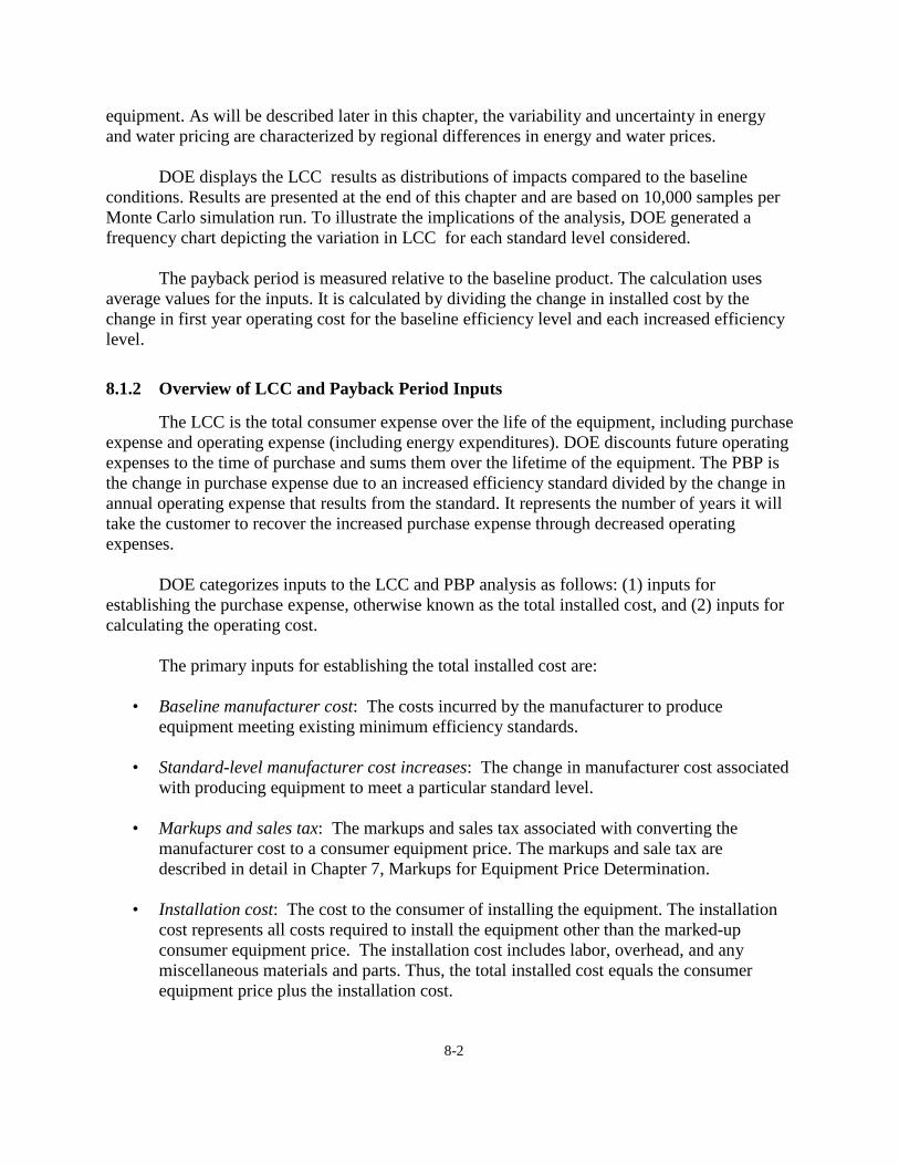
before O&P) and installation costs including O&P. DOE determined that installation costs would not be impacted with increased standard levels. Table 8.2.7 Commercial Clothes Washers: Baseline Installation Costs Bare Costs (2013$) Including Overhead & Profit (2013$)
Installation Type Material Labor Total Total Material* Labor**
Average $1,250 $149 $1,399 $1,600 $1,374 $225
Average (2013$) $225 * Material costs including O&P equal bare costs plus 10% profit. ** DOE derived labor cost including O&P by subtracting material with O&P from total with O&P. Source: RS Means, Mechanical Cost Data, 2013.
8.2.1.6 Total Installed Cost
The total installed cost is the sum of the consumer equipment price and the installation cost. Refer back to section 8.2.1 to see the equations that DOE used to calculate the total installed cost for baseline and standard-level products. Table 8.2.8 and Table 8.2.9 present the consumer equipment price, installation costs, and total installed costs for top-loading and front-loading washers, respectively. Prices and costs are presented at the baseline level and each standard level. Table 8.2.8 Top-Loading Commercial Clothes Washers: Consumer Equipment Prices,
Installation Costs, and Total Installed Costs
Efficiency Level
Modified Energy Factor
(cu.ft./kWh/cyc)
Integrated Water Factor
(gal/cu.ft.)
Equipment Price
(2013$)
Installation Cost
(2013$)
Total Installed Cost
(2013$)
Baseline 1.15 8.90 $1,004 $225 $1,229 1 1.35 8.80 $1,004 $225 $1,229 2 1.55 6.90 $1,068 $225 $1,293
8-11

Table 8.2.9 Front-Loading Commercial Clothes Washers: Consumer Equipment Prices, Installation Costs, and Total Installed Costs
Efficiency Level
Modified Energy Factor
(cu.ft./kWh/cyc)
Integrated Water Factor
(gal/cu.ft.)
Equipment Price
(2013$)
Installation Cost
(2013$)
Total Installed Cost
(2013$)
Baseline 1.65 5.20 $1,592 $225 $1,817 1 1.80 4.50 $1,592 $225 $1,817 2 2.00 4.10 $1,593 $225 $1,818 3 2.20 3.90 $1,623 $225 $1,848
8.2.1.7 Future Product Prices
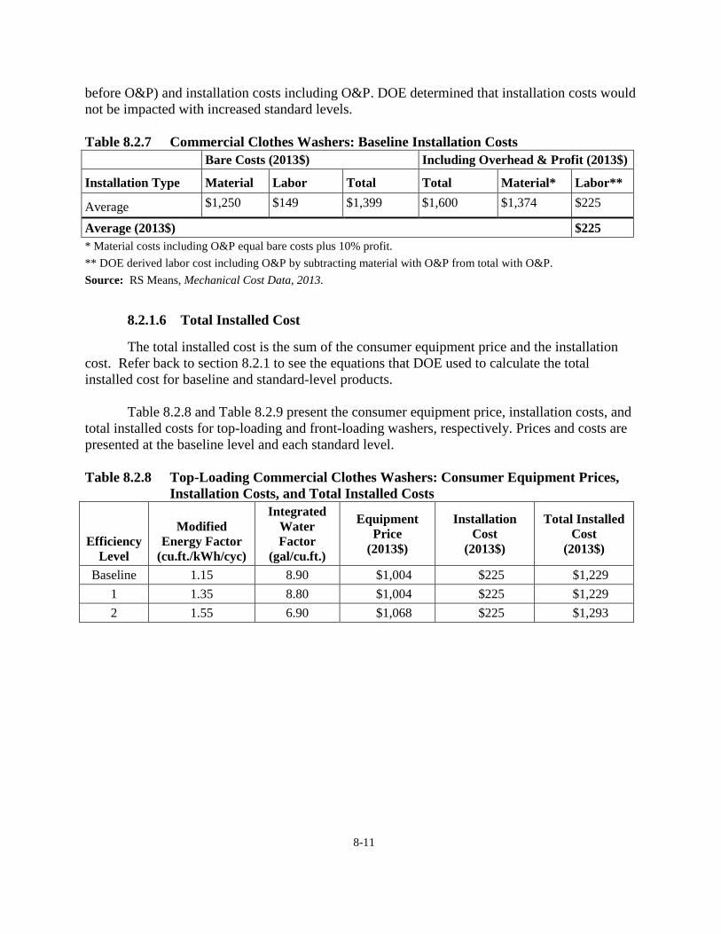
DOE obtained historical PPI data for commercial laundry and drycleaning machinery spanning the time period 1982-2013 from the Bureau of Labor Statistics’ (BLS).a The PPI data reflect nominal prices, adjusted for product quality changes. An inflation-adjusted (deflated) price index for commercial laundry and drycleaning machinery was calculated by dividing the PPI series by the Gross Domestic Product Chained Price Index (see Figure 8.2.1).
a Series ID PCU3333183333182; http://www.bls.gov/ppi/
8-12
Figure 8.2.1 Historic Nominal and Deflated Producer Price Indexes for
Commercial Laundry and Drycleaning Machinery From the early-1980s to early-1990s, the deflated price index for commercial laundry and drycleaning machinery was decreasing slowy. Since 1993, the deflated price index for this industry has risen consistently and only till the last forth year (2010), the prices started to stay flat and dropped slightly in 2013. The rising prices we observed in commercial laundry and drycleaning machinery industry from early-2000s to 2010 could partly attribute to the concurrent price increase in copper and steel products which are heavily used in commercial clothes washers; however, it is uncertain what was cauing the price to rise between 1993 to early-2000s. Although the prices in this industry remain roughly constant in the last three years, given the uncertain cuase of the long-lasting increasing price trend and the slowdown in global economic activity in recent years, DOE believes that the extent to how the trends will continue is very uncertain. Additionally, in terms of the types of commerial clothes washers considered in this rulemaking, they are largely similar to the residential clothes washers. Hence, DOE also referred to the household laundry equipment PPI for comparison and found that the deflated household laundry equipment PPI have actually been decreasing consistenly from 1947 to 2013 but the decreasing rate has slowed down in recent years, as shown in Figure 8.2.2. b
b Series ID PCU335224335224P; http://www.bls.gov/ppi/
8-13

Figure 8.2.2 Historic Nominal and Deflated Producer Price Indexes for
Household Laundry Equipment
Given the uncertainties mentioned above, DOE decided to use constant prices as the default price assumption to project future commercial clothes washer prices. Thus, projected prices for the LCC and PBP analysis are equal to the 2013 values for each efficiency level in each product class.
8.2.2 Operating Cost Inputs
DOE defines the operating cost by the following equation:
MCRCWCECOC +++= where:
EC = Energy expenditure associated with operating the equipment, WC = For dishwashers and commercial clothes washers, the water expenditure
associated with operating the equipment, RC = Repair cost associated with component failure, and MC = Service cost for maintaining equipment operation.
Table 8.2.10 shows the inputs for determining the operating costs. The inputs listed in Table 8.2.10 are also necessary for determining lifetime operating expenses, which include the
8-14

energy price trends (and water price trends), product lifetime, discount rate, and effective date of the standard.
Table 8.2.10 Inputs for Operating Cost Annual Energy (and Water) Consumption
Energy and Water Prices
Repair and Maintenance Costs
Energy and Water Price Trends
Product Lifetime
Discount Rate
Effective Date of Standard The annual energy consumption is the site energy use associated with operating the equipment. The annual water consumption, which is applicable to commercial clothes washers, is the site water use associated with operating the equipment. The annual energy (and water) consumption vary with the product efficiency. That is, the energy and water consumption associated with standard-level equipment (i.e., equipment with efficiencies greater than baseline equipment) are less than the consumptions associated with baseline equipment. Energy and water prices are the prices paid by consumers for energy (i.e., electricity, gas, or oil) and water. Multiplying the annual energy and water consumption by the energy and water prices yields the annual energy cost and water cost, respectively. Repair costs are associated with repairing or replacing components that have failed. Maintenance costs are associated with maintaining the operation of the equipment. DOE used energy and water price trends to forecast energy and water prices into the future and, along with the product lifetime and discount rate, to establish the lifetime energy and water costs. The product lifetime is the age at which the equipment is retired from service. The discount rate is the rate at which DOE discounted future expenditures to establish their present value. DOE calculated the operating cost for baseline products based on the following equation:
BASEBASEWATERBASEENERGYBASE
BASEBASEBASEBASEBASE
MCRCPRICEAWCPRICEAECMCRCWCECOC
++×+×=+++=
where:
OCBASE = Baseline operating cost, ECBASE = Energy expenditure associated with operating the baseline equipment, WCBASE = For commercial clothes washers, the water expenditure associated with
operating the baseline equipment, RCBASE = Repair cost associated with component failure for the baseline
equipment, MCBASE = Service cost for maintaining baseline equipment operation,
8-15

AECBASE = Annual energy consumption for baseline equipment, PRICEENERGY = Energy price, AWCBASE = Annual water consumption for baseline equipment, and PRICEWATER = Water price.
DOE calculated the operating cost for standard-level products based on the following equation:
( ) ( )( ) ( )STDBASESTDBASE
WATERSTDBASEENERGYSTDBASE
STDSTDWATERSTDENERGYSTD
STDSTDSTDSTDSTD
MCMCRCRCPRICEAWCAWCPRICEAECAEC
MCRCPRICEAWCPRICEAECMCRCWCECOC
D++D++×D+×D=
++×+×=+++=
____
where:
OCSTD = Standard-level operating cost, ECSTD = Energy expenditure associated with operating standard-level equipment, WCSTD = For commercial clothes washers, the water expenditure associated with
operating standard-level equipment, RCSTD = Repair cost associated with component failure for standard-level
equipment, MCSTD = Service cost for maintaining standard-level equipment operation, AECSTD = Annual energy consumption for standard-level equipment, PRICEENERGY = Energy price, AWCSTD = Annual water consumption for standard-level equipment, PRICEWATER = Water price, ΔAECSTD = Change in annual energy consumption caused by standard-level
equipment, ΔAWCSTD = Change in annual water consumption caused by standard-level
equipment, ΔRCSTD = Change in repair cost caused by standard-level equipment, and ΔMCSTD = Change in maintenance cost caused by standard-level equipment.
The remainder of this section provides information about each of the above input variables that DOE used to calculate the operating costs for cooking products, dishwashers, dehumidifiers, and commercial clothes washers.
8.2.2.1 Annual Energy and Water Consumption
Chapter 7, Energy and Water Use Analysis, details how DOE determined the annual energy and water consumption for baseline and standard-level products. DOE characterized the variability of commercial clothes washer usage based on several studies. For both multi-family as well as laundromat applications, DOE equally weighted each
8-16

study to establish the variability. Refer back to Chapter 7, section 7.4 to review how DOE characterized commercial clothes washer usage variability. The tables presented below are based on the energy and water use analysis described in Chapter 7. Keep in mind that the annual energy and water consumption values in the tables below are averages. DOE captured the variability in energy (and water) consumption when it conducted its LCC and PBP analysis. Table 8.2.11 and Table 8.2.12 provide the average annual energy and water consumption by efficiency level for top-loading commercial clothes washers. Table 8.2.13 and Table 8.2.14 provide the average annual energy and water consumption by efficiency level for front-loading commercial clothes washers. DOE presents annual consumption based on two applications: multi-family housing and laundromats. Table 8.2.11 Top-Loading Commercial Clothes Washers, Multi-Family Application:
Annual Energy and Water Use by Efficiency Level
Efficiency Level
MEF IWF
Annual Energy Use*
Annual Water Use
Water Heating** Drying*** Machine Electric Gas Electric Gas
cu.ft./kWh/cyc gal/cu.ft. kWh/yr MMBtu/yr kWh/yr MMBtu/yr kWh/yr 1000 gal/year Baseline 1.15 8.90 107.1 1.29 913.0 5.23 240.9 30.21
1 1.35 8.80 138.6 1.68 692.0 3.97 230.0 29.87 2 1.55 6.90 108.7 1.31 690.9 3.96 109.5 24.26
* Annual usage based on 3.0 cycles per day (1,095 cycles per year). ** Electric and gas water heating based on water heater efficiencies of 98% for electric and 83% for gas. Water
heater consumption is weighted by the share of buildings with electric (25%) and gas (75%) water heaters. *** Dryer consumption is weighted by the share of buildings with electric (40%) and gas (60%) dryers.
Table 8.2.12 Top-Loading Commercial Clothes Washers, Laundromat Application:
Annual Energy and Water Use by Efficiency Level
Efficiency Level
MEF IWF
Annual Energy Use*
Annual Water Use
Water Heating** Drying*** Machine Electric Gas Electric Gas
cu.ft./kWh/cyc gal/cu.ft. kWh/yr MMBtu/yr kWh/yr MMBtu/yr kWh/yr 1000 gal/year Baseline 1.15 8.90 0.0 2.36 0.0 11.92 329.3 41.30
1 1.35 8.80 0.0 3.05 0.0 9.04 314.4 40.84 2 1.55 6.90 0.0 2.39 0.0 9.02 149.7 33.17
* Annual usage based on 4.1 cycles per day (1,497 cycles per year). ** Electric and gas water heating based on water heater efficiencies of 98% for electric and 83% for gas. Water
heater consumption is weighted by the share of buildings with electric (0%) and gas (100%) water heaters. *** Dryer consumption is weighted by the share of buildings with electric (0%) and gas (100%) dryers.
8-17

Table 8.2.13 Front-Loading Commercial Clothes Washers, Multi-Family Application: Annual Energy and Water Use by Efficiency Level
Efficiency Level
MEF IWF
Annual Energy Use*
Annual Water Use
Water Heating** Drying*** Machine Electric Gas Electric Gas
cu.ft./kWh/cyc gal/cu.ft. kWh/yr MMBtu/yr kWh/yr MMBtu/yr kWh/yr 1000 gal/year Baseline 1.65 5.20 88.9 1.07 552.9 3.17 120.5 15.94
1 1.80 4.50 91.1 1.10 516.1 2.96 87.6 14.10 2 2.00 4.10 51.4 0.62 501.3 2.87 109.5 12.85 3 2.20 3.90 67.1 0.81 522.7 3.00 76.7 14.12
* Annual usage based on 3.0 cycles per day (1,095 cycles per year). ** Electric and gas water heating based on water heater efficiencies of 98% for electric and 83% for gas. Water
heater consumption is weighted by the share of buildings with electric (25%) and gas (75%) water heaters. *** Dryer consumption is weighted by the share of buildings with electric (40%) and gas (60%) dryers.
Table 8.2.14 Front-Loading Commercial Clothes Washers, Laundromat Application:
Annual Energy and Water Use by Efficiency Level
Efficiency Level
MEF IWF
Annual Energy Use*
Annual Water Use
Water Heating** Drying*** Machine Electric Gas Electric Gas
cu.ft./kWh/cyc gal/cu.ft. kWh/yr MMBtu/yr kWh/yr MMBtu/yr kWh/yr 1000 gal/year Baseline 1.65 5.20 0.0 1.96 0.0 7.22 164.7 21.80
1 1.80 4.50 0.0 2.01 0.0 6.74 119.8 19.28 2 2.00 4.10 0.0 1.13 0.0 6.55 149.7 17.57 3 2.20 3.90 0.0 1.48 0.0 6.83 104.8 19.30
* Annual usage based on 4.1 cycles per day (1,497 cycles per year). ** Electric and gas water heating based on water heater efficiencies of 98% for electric and 83% for gas. Water
heater consumption is weighted by the share of buildings with electric (0%) and gas (100%) water heaters. *** Dryer consumption is weighted by the share of buildings with electric (0%) and gas (100%) dryers.
8.2.2.2 Energy and Water Prices
DOE derived energy prices for 27 geographic areas in the U.S. and derived water prices
for the four Census regions. Using these data, DOE analyzed the variability of energy and water prices at the regional level for commercial clothes washers. DOE characterized energy and water price regional variability with probability distributions. It based the probability associated with each regional energy and water price on the population weight of each region.
8-18

The methodology that DOE used for deriving the energy and water prices is presented below. Included are tables that summarize the regional energy and water prices for each product.
Energy Prices DOE derived average commercial electricity prices from data that are published annually based on EIA Form 861.2 Those data include annual electricity sales in kilowatt-hours, revenues from electricity sales, and number of customers in the residential, commercial, and industrial sectors, for every utility serving final consumers. DOE calculated commercial electricity prices for each of the 27 U.S. geographic areas to accordance with RECS 2009 geographic areas. The calculation of an average commercial electricity price proceeds in two steps:
1. For each utility, estimate an average commercial price by dividing the commercial revenues by commercial sales.
2. Calculate a regional average price, weighting each utility with customers in a region by the number of commercial consumers served in that region.
Table 8.2.15 shows the results for each geographic region.
8-19

Table 8.2.15 Average Commercial Electricity Prices in 2012 Geographic Area 2012$/kWh
1 Connecticut, Maine, New Hampshire, Rhode Island, Vermont 0.138
2 Massachusetts 0.143 3 New York 0.156 4 New Jersey 0.133 5 Pennsylvania 0.106 6 Illinois 0.089 7 Indiana, Ohio 0.098 8 Michigan 0.114 9 Wisconsin 0.105
10 Iowa, Minnesota, North Dakota, South Dakota 0.087
11 Kansas, Nebraska 0.096 12 Missouri 0.085 13 Virginia 0.085
14 Delaware, District of Columbia, Maryland, West Virginia 0.109
15 Georgia 0.099 16 North Carolina, South Carolina 0.092 17 Florida 0.099 18 Alabama, Kentucky, Mississippi 0.100 19 Tennessee 0.106 20 Arkansas, Louisiana, Oklahoma 0.080 21 Texas 0.097 22 Colorado 0.095 23 Idaho, Montana, Utah, Wyoming 0.082 24 Arizona 0.100 25 Nevada, New Mexico 0.094 26 California 0.140 27 Alaska , Hawaii , Oregon, Washington 0.108 Source: EIA Form 861. Table 8.2.16 shows the national average commercial electricity prices for commercial clothes washers based on the relative residential consumer weight of each geographic area. DOE used 2013 population estimates from the U.S. Census as a proxy to estimate how the national saturation of commercial clothes washers was distributed over the 27 geographic areas.3 Because DOE conducted the LCC and PBP analysis in 2013$, all electricity prices are in 2013$. To perform the necessary monetary conversion, DOE used the CPI to convert the electricity prices from 2012$ to 2013$.
8-20

Table 8.2.16 Average Commercial Electricity Prices for Commercial Clothes Washers in
2013 Geographic Area 2013$/kWh Saturation
1 Connecticut, Maine, New Hampshire, Rhode Island, Vermont $0.140 2.5%
2 Massachusetts $0.145 2.1% 3 New York $0.159 6.2% 4 New Jersey $0.135 2.8% 5 Pennsylvania $0.108 4.0% 6 Illinois $0.091 4.1% 7 Indiana, Ohio $0.099 5.7% 8 Michigan $0.115 3.1% 9 Wisconsin $0.107 1.8%
10 Iowa, Minnesota, North Dakota, South Dakota $0.088 3.2%
11 Kansas, Nebraska $0.098 1.5% 12 Missouri $0.086 1.9% 13 Virginia $0.087 2.6%
14 Delaware, District of Columbia, Maryland, West Virginia $0.111 2.4%
15 Georgia $0.101 3.2% 16 North Carolina, South Carolina $0.093 4.6% 17 Florida $0.100 6.2% 18 Alabama, Kentucky, Mississippi $0.102 3.9% 19 Tennessee $0.107 2.1% 20 Arkansas, Louisiana, Oklahoma $0.081 3.6% 21 Texas $0.099 8.4% 22 Colorado $0.097 1.7% 23 Idaho, Montana, Utah, Wyoming $0.083 1.9% 24 Arizona $0.101 2.1% 25 Nevada, New Mexico $0.096 1.5% 26 California $0.142 12.1% 27 Alaska , Hawaii , Oregon, Washington $0.110 4.7% Source: EIA Form 861.
Commercial Natural Gas Prices DOE obtained the data for the natural gas price calculation from the EIA publication Natural Gas Prices.4 This publication includes a compilation of monthly natural gas delivery volumes and average consumer prices by State, for residential, commercial, and industrial customers. The Department used the complete annual data for 2012 to calculate an average annul price for each area. The calculation of average prices proceeds in two steps:
8-21

1. Calculate the annual price for each State using a simple average over the appropriate
months. 2. Calculate a regional price, weighting each State in a region by its population.
This method differs from the method used to calculate electricity prices because EIA does not provide consumer- or utility-level data on gas consumption and prices. Table 8.2.17 shows the national average commercial natural gas prices for commercial clothes washers based on the relative commercial consumer weight of each geographic area. DOE used 2013 population estimates from the U.S. Census as a proxy to estimate how the national saturation of commercial clothes washers was distributed over the 27 geographic areas. DOE also used the CPI to convert the natural gas prices from 2012$ to 2013$.
8-22

Table 8.2.17 Average Commercial Natural Gas Prices in 2012 Geographic Area 2013$/MMBtu Saturation
1 Connecticut, Maine, New Hampshire, Rhode Island, Vermont $10.21 2.5%
2 Massachusetts $10.20 2.1% 3 New York $7.38 6.2% 4 New Jersey $8.29 2.8% 5 Pennsylvania $10.54 4.0% 6 Illinois $8.76 4.1% 7 Indiana, Ohio $7.46 5.7% 8 Michigan $8.64 3.1% 9 Wisconsin $6.92 1.8%
10 Iowa, Minnesota, North Dakota, South Dakota $6.49 3.2%
11 Kansas, Nebraska $8.25 1.5% 12 Missouri $10.44 1.9% 13 Virginia $8.70 2.6%
14 Delaware, District of Columbia, Maryland, West Virginia $10.97 2.4%
15 Georgia $9.84 3.2% 16 North Carolina, South Carolina $8.47 4.6% 17 Florida $10.19 6.2% 18 Alabama, Kentucky, Mississippi $9.85 3.9% 19 Tennessee $8.27 2.1% 20 Arkansas, Louisiana, Oklahoma $8.88 3.6% 21 Texas $6.75 8.4% 22 Colorado $7.68 1.7% 23 Idaho, Montana, Utah, Wyoming $7.22 1.9% 24 Arizona $9.49 2.1% 25 Nevada, New Mexico $6.98 1.5% 26 California $6.97 12.1% 27 Alaska , Hawaii , Oregon, Washington $13.08 4.7% Source: EIA, Natural Gas Prices.
8-23
Water Prices DOE obtained water price data from the year 2012 from the Water and Wastewater Rate Survey conducted by Raftelis Financial Consultants and the American Water Works Association.5 The survey covers approximately 290 water utilities and 214 wastewater utilities, with each industry analyzed separately. The water survey includes, for each utility, the cost to consumers of purchasing a given volume of water. In this case, the data include a division of the total consumer cost into fixed and volumetric charges. The calculations use only the volumetric charge to calculate water prices, since only this charge would be affected by a change in water consumption. Including the fixed charge in the average would lead to a slightly higher water price. The Water and Wastewater Rate Survey provides prices separately for residential and non-residential customers. For wastewater utilities, the format is similar, but the cost refers to the cost of treating a given volume of wastewater. In both surveys, the non-residential sector is divided into four sub-sectors based on the average monthly volume of water delivered or, equivalently, the size of the delivery pipe. The sub-sectors are named non-manufacturing, commercial, industrial 1, and industrial 2. DOE’s analysis uses the commercial category to estimate prices for commercial consumers. A sample of 290 utilities is not large enough to calculate regional prices for all U.S. Census divisions and large States (for comparison, the EIA Form 861 data include more than 3000 utilities). For this reason, DOE calculated regional values at the Census region level (Northeast, South, Midwest, and West). The calculation of average per-unit-volume prices proceeds in three steps:
1. For each utility, calculate the per-unit-volume price by dividing the total volumetric cost by the volume delivered.
2. Calculate a State-level average price by weighting each utility in a given State by the number of commercial consumers it serves.
3. Calculate a regional average by combining the State-level averages, weighting each by the population of that State. This third step helps reduce any bias in the sample that may occur due to relative under-sampling of large States.
The results of the calculation for the commercial sector are presented in Table 8.2.18. The price units in the table are dollars per thousand gallons ($/tg).
8-24

Table 8.2.18 Average Per-Unit-Volume Water and Waste Water Prices in 2012 Commercial Region 2013$/tg Water 2013$/tg Wastewater Northeast 3.90 6.58 Midwest 3.32 3.97 South 3.33 4.74 West 4.04 4.76
Source: Raftelis, Raftelis Survey, 2013.
8.2.2.3 Energy and Water Price Trends
DOE used price forecasts by the EIA to estimate the trends in natural gas, oil, and electricity prices. To arrive at prices in future years, it multiplied the average prices described in the preceding section (section 8.2.2.2) by the forecast of annual average price changes in EIA’s AEO 2014.6 To estimate the trend after 2040, DOE followed past guidelines provided to the Federal Energy Management Program (FEMP) by EIA and used the average rate of change during 2030–2040. The Department set up its analysis to calculate LCC and PBP using three separate projections: Reference, Low Economic Growth, and High Economic Growth. These three cases reflect the uncertainty of economic growth in the forecast period. The high and low growth cases show the projected effects of alternative growth assumptions on energy markets. Figure 8.2.3 and Figure 8.2.4 show the commercial electricity and natural gas price trends, respectively, based on the three projections. For the LCC results presented in section 8.4, DOE used only the energy price forecasts from the AEO 2014 Reference Case.
8-25

Figure 8.2.3 Electricity Price Trends
Figure 8.2.4 Natural Gas Price Trends
To estimate the future trend for water and wastewater prices, DOE used data on the historic trend in the national water price index (U.S. city average) from 1970 through 2012.7 DOE extrapolated the future trend based on the linear growth from 1970 to 2012. But rather than use the extrapolated trend to forecast the prices for the eight years after 2012, DOE used the
0.90
0.95
1.00
1.05
1.10
1.15
1.20
1.25
1.30El
ectr
icity
Pric
e Tr
end
(201
2=10
0)
Reference High Low
0.90
1.10
1.30
1.50
1.70
1.90
2.10
2.30
Nat
ural
Gas
Pric
e Tr
end
(201
2=10
0)
Reference Case High Case Low Case
8-26

annual growth rate between 2012 and 2021 to project water price trend. Otherwise, forecasted prices for this eight-year time period would have been much lower than the price in 2012. Beyond the eight-year time period, DOE used the extrapolated trend to forecast prices out to the year 2047. Figure 8.2.5 shows the historical and projected water price trend data. DOE used the forecasted data to estimate water and wastewater prices for commercial clothes washers.
Figure 8.2.5 Water Price Trend
8.2.2.4 Repair and Maintenance Costs
Typically, small incremental changes in product efficiency incur no, or only very small, changes in repair and maintenance costs over baseline products. However, equipment with efficiencies that are significantly higher than the baseline are more likely to incur higher repair and maintenance costs because its higher complexity and higher part count typically increases the cumulative probability of failure. The Whirlpool Corporation estimates that the unit shipments of horizontal-axis commercial clothes washers are less than half that of vertical-axis machines while their in-warranty repair costs are double that of vertical-axis machines.8 This suggests that the repair of horizontal-axis machines is four times as costly as that of vertical-axis machines. Because in-warranty repair costs, based on Whirlpool’s experience, are greater for horizontal-axis machines that vertical-axis machines, DOE estimated that commercial clothes washer repair costs would increase as a function of equipment efficiency. DOE utilized an algorithm developed for central air conditioners and heat pumps to estimate repair cost increases.9 This algorithm calculates annualized repair costs by dividing the half the equipment retail price by the equipment lifetime as show in the expression below:
y = 8.502x - 16753R² = 0.9558
0.0
100.0
200.0
300.0
400.0
500.0
600.0
700.0
800.0 Water Price CPI Trend (1982-1984=100)
Historical Water Price CPI
Extrapolated Water Price CPI TrendLinear (Historical Water Price CPI)
8-27

LIFEEQPRC ANNUAL
×=
5.0
where:
RCANNUAL = Annualized repair cost associated with equipment, EQP = Consumer equipment price, and LIFE = Product lifetime.
Table 8.2.19 and Table 8.2.20 show for each product class and each product application (multi-family buildings and laundromats) the annualized repair costs for the commercial clothes washer baseline and efficiency levels. Annualized repair costs for each product application differ because commercial clothes washer lifetime is different for each application. (Product lifetimes are presented below is section 8.2.3). The tables also present the consumer equipment prices for the baseline level and each efficiency level. Table 8.2.19 Top-Loading Commercial Clothes Washer Annualized Repair Costs
Efficiency Level
Modified Energy Factor
(cu.ft./kWh/cyc)
Integrated Water Factor
(gal/cu.ft.)
Equipment Price
(2013$)
Annualized Repair Cost (2013$)
Multi-Family* Laundromat*
Baseline 1.15 8.90 $1,004 $46 $71 1 1.35 8.80 $1,004 $46 $71 2 1.55 6.90 $1,068 $49 $76
* Average product lifetime: Multi-family = 11.3 years; Laundromat = 7.1 years. Table 8.2.20 Front-Loading Commercial Clothes Washer Annualized Repair Costs
Efficiency Level
Modified Energy Factor
(cu.ft./kWh/cyc)
Integrated Water Factor
(gal/cu.ft.)
Equipment Price
(2013$)
Annualized Repair Cost (2013$)
Multi-Family* Laundromat*
Baseline 1.65 5.20 $1,592 $72 $113 1 1.80 4.50 $1,592 $72 $113 2 2.00 4.10 $1,593 $73 $113 3 2.20 3.90 $1,623 $74 $115
* Average product lifetime: Multi-family = 11.3 years; Laundromat = 7.1 years.
8.2.3 Product Lifetime
DOE used only primary sources of data to estimate product lifetimes. DOE considered the sources listed in Table 8.2.21 to estimate product lifetime.
8-28

Table 8.2.21 Commercial Clothes Washers: Product Lifetime Estimates and Sources Lifetime (years) Source 7 to 10 CEE (1998) 5 Top-Loading (12 to 14 lbs.): 5 to 8* Front-Loading (18 to 50 lbs.): 10 to 15** CLA10
8 to 9*** ACEEE (2001)11 5 (high-use)* to 13 (low-use)** Southern California Edison (2000)12 15** † CALMAC (2000)13 * Used to establish laundromat lifetime only. ** Used to establish multi-family lifetime only. *** Depending on the usage rate, the life can be shorter. † Based on engineering judgment.
Because DOE conducted the LCC analysis based on analyzing two product applications—multi-family and laundromats—it established separate lifetimes for each product application. Because clothes washers in multi-family applications are used less frequently than in laundromats, DOE decided to use only those sources that indicated lifetimes of seven years or greater for multi-family applications. For laundromat applications, where clothes washers receive heavier use, DOE decided to use only those sources that indicated lifetimes of 10 years or less. DOE then took an average of the lifetime estimates that met the above criteria. For multi-family applications the average lifetime turned out to be 11.3 years, while the average lifetime for laundromats was 7.1 years. DOE used the low estimate for the above applicable sources to establish the minimum product lifetime for each product application. For multi-family applications the minimum estimate is 7 years and for laundromats it is 5 years. To establish the maximum product lifetime, DOE took the difference between the minimum and average values (4.3 years for multi-family and 2.1 years for laundromats) and added it to the average product lifetime. The minimum, average, and maximum lifetime estimates for each product application are shown in Table 8.2.22. Table 8.2.22 Commercial Clothes Washers: Average, Minimum, and Maximum Product
Lifetimes
Product Minimum
years Average
years Maximum
years Multi-Family Laundromats
7.0 5.0
11.3 7.1
15.5 9.3
DOE characterized the clothes washer product lifetimes for each product application with Weibull distributions. Appendix 8C presents the Weibull distributions for commercial clothes washers that DOE used in the LCC and PBP analysis.
8-29
8.2.4 Discount Rates
The commercial discount rate is the rate at which future operating costs are discounted to establish their present value in the LCC analysis. The discount rate value is applied in the LCC to future year energy costs and non-energy operations and maintenance costs to calculate the estimated net life-cycle cost of products of various efficiency levels and life-cycle cost savings as compared to the baseline for a representative sample of commercial end users.
DOE’s method views the purchase of a higher efficiency appliance as an investment that
yields a stream of energy cost savings. DOE derived the discount rates for the LCC analysis by estimating the cost of capital for companies that purchase commercial clothes washers. The weighted average cost of capital (WACC) is commonly used to estimate the present value of cash flows to be derived from a typical company project or investment. Most companies use both debt and equity capital to fund investments, so their cost of capital is the weighted average of the cost to the firm of equity and debt financing, as estimated from financial data for publicly traded firms in the sectors that purchase commercial clothes washers.14 Damodaran Online is a widely used source of information about company debt and equity financing for most types of firms, and was the primary source of data for two sectors included in this analysis: property management and lodging.15 The Damodaran database does not include data on the personal services sector, which includes laundromats, or public sectors, such as state-run educational facilities. Discount rates for laundromats were estimated using sector-level financial data for the personal services sector published by Ibbotson Associates. 16 Ibbotson Associates is a leading authority on asset allocation with expertise in capital market expectations and portfolio implementation. DOE used the average state and local bond rate to represent the discount rate for education.17 DOE estimated the cost of equity using the capital asset pricing model (CAPM).18 The CAPM assumes that the cost of equity (ke) for a particular company is proportional to the systematic risk faced by that company, where high risk is associated with a high cost of equity and low risk is associated with a low cost of equity. The systematic risk facing a firm is determined by several variables: the risk coefficient of the firm (β), the expected return on risk-free assets (Rf), and the equity risk premium (ERP). The risk coefficient of the firm indicates the risk associated with that firm relative to the price variability in the stock market. The expected return on risk-free assets is defined by the yield on long-term government bonds. The ERP represents the difference between the expected stock market return and the risk-free rate. The cost of equity financing is estimated using the following equation, where the variables are defined as above:
( )ERPRk fe ×+= β
Where:
ke = cost of equity, Rf = expected return on risk-free assets,
8-30

β = risk coefficient of the firm, and ERP = equity risk premium.
Several parameters of the cost of capital equations can vary substantially over time, and therefore the estimates can vary with the time period over which data is selected and the technical details of the data averaging method. For guidance on the time period for selecting and averaging data for key parameters and the averaging method, DOE used Federal Reserve methodologies for calculating these parameters. In its use of the CAPM, the Federal Reserve uses a forty-year period for calculating discount rate averages, utilizes the gross domestic product price deflator for estimating inflation, and considers the best method for determining the risk free rate as one where “the time horizon of the investor is matched with the term of the risk-free security.”19 By taking a forty-year geometric average of Federal Reserve data on annual nominal returns for 10-year Treasury bills, DOE estimated the following risk free rates for 2004 - 2013 (Table 8.2.23).20 DOE also estimated the ERP by calculating the difference between risk free rate and stock market return for the same time period, as estimated using Damodaran Online data on the historical return to stocks.21 Table 8.2.23 Risk free rate and equity risk premium, 2004 – 2013
Year Risk free rate (%) ERP (%) 2004 7.10% 3.25%
2005 7.11% 3.68%
2006 7.10% 3.49%
2007 7.08% 3.36%
2008 7.01% 2.40%
2009 6.88% 3.07%
2010 6.74% 3.23%
2011 6.61% 2.94%
2012 6.41% 3.99%
2013 6.24% 5.30% The cost of debt financing (kd) is the interest rate paid on money borrowed by a company. The cost of debt is estimated by adding a risk adjustment factor (Ra) to the risk-free rate. This risk adjustment factor depends on the variability of stock returns represented by standard deviations in stock prices. So for firm i, the cost of debt financing is:
aifdi RRk += Where:
8-31

kd = cost of debt financing for firm, i, Rf = expected return on risk-free assets, and Rai = risk adjustment factor to risk-free rate for firm, i.
DOE estimates the WACC using the following equation:
ddee wkwkWACC ×+×= Where:
WACC = weighted average cost of capital, we = proportion of equity financing, and wd = proportion of debt financing.
By adjusting for the influence of inflation, DOE estimates the real weighted average cost of capital, or discount rate, for each company. DOE then aggregates the company real weighted average costs of capital to estimate the discount rate for each of the ownership types in the commercial clothes washer analysis. Table 8.2.24 shows the average WACC values for the major sectors that purchase commercial clothes washers. While WACC values for any sector may trend higher or lower over substantial periods of time, these values represent a cost of capital that is averaged over major business cycles. Table 8.2.24 Weighted Average Cost of Capital for Sectors that Purchase Washers
Sector Real Weighted Average Cost of Capital (%)
Standard Deviation (%)
Property 5.12% 0.90%
Lodging 5.96% 1.65%
Education 2.46% 2.15%
Personal Services a 4.67% -- a The Ibbotson Associates report provides only a single value for the personal services sector, so a standard deviation cannot be calculated.
8.2.5 Effective Date of Standard
The effective date is the future date when a new standard becomes operative. Based on DOE’s implementation report for energy conservation standards activities submitted pursuant to Section 136 of the Energy Policy Act of 2005, a final rule for the commercial clothes washers being considered for this standards rulemaking is scheduled for completion no later than January 1, 2015. Therefore, the effective date of any new energy efficiency standards for these products
8-32

will be three years after the final rule is published, which is January 1, 2018. The Department calculated the LCC for all consumers as if they each would purchase a new piece of equipment in the year the standard takes effect.
8.2.6 Equipment Assignment for the Base Case
For purposes of conducting the LCC analysis, DOE analyzed standard levels relative to a baseline efficiency level. However, some consumers already purchase products with efficiencies greater than the baseline levels. Thus, to accurately estimate the percentage of consumers that would be affected by a particular standard level, DOE took into account the distribution of product efficiencies currently in the marketplace. In other words, rather than analyzing the impacts of a particular standard level assuming that all consumers are currently purchasing products at the baseline level, DOE conducted the analysis by taking into account the full breadth of product efficiencies that consumers purchase under the base case (i.e., the case without new energy efficiency standards).
DOE took into account the mix of commercial clothes washer efficiencies by
characterizing the current mix of product efficiencies as a probability distribution. In other words, as DOE performed the Monte Carlo simulation, each standard level analyzed was evaluated against the distribution of product efficiencies in the base case. For top-loading commercial clothes washers, DOE utilized the market share efficiency data for 2010-2013 submitted by AHAM to establish the base-case efficiency distributions for 2013.22 The market share efficiency distribution for top-loading units submitted by AHAM provided a consolidated share for baseline (1.15 MEFJ2) and levels higher than the baseline. In order to accurately represent the higher efficiency levels through appropriate market shares, the analysis utilized available models data from DOE’s Compliance Certification Database for commercial clothes washers to allocate shares to higher efficiency levels.23 For front-loading washers, DOE used the data submitted by AHAM for 2013. DOE used the 2013 distribution to represent the market in the compliance year (2018). DOE found that the distribution based on Energy Star qualified products matched closely with the data submitted by AHAM.24 Table 8.2.25 and Table 8.2.26 present the market shares of the efficiency levels in the base case for top-loading and front-loading washers, respectively. The tables represent the equipment that establishments would have purchased in the year 2018 in the absence of new standards. Table 8.2.25 Top-Loading Commercial Clothes Washers: Base Case Market Shares
Efficiency Level MEF IWF Market Share Baseline 1.15 8.90 62.0%*
1 1.35 8.80 26.7%** 2 1.55 6.90 11.3%***
* Represents units with the following MEF and WF ratings: 1.15≤ MEF < 1.35; 8.9 ≥ IWF > 8.8. ** Represents units with the following MEF and WF ratings: 1.35 ≤ MEF < 1.55; 8.8 ≥ IWF > 6.9.
8-33

*** Represents units with the following MEF and WF ratings: MEF ≥ 1.55; IWF ≤ 6.9. Table 8.2.26 Front-Loading Commercial Clothes Washers: Base Case Market Shares
Efficiency Level MEF WF Market Share Baseline 1.65 5.20 0.0%*
1 1.80 4.50 31.0%** 2 2.00 4.10 69.0%*** 3 2.20 3.90 0.0%†
* Represents units with the following MEF and WF ratings: 1.65 ≤ MEF < 1.80; 5.2 ≥ IWF > 4.5. ** Represents units with the following MEF and WF ratings: 1.80 ≤ MEF < 2.00; 4.5 ≥ IWF > 4.1. *** Represents units with the following MEF and WF ratings: 2.00 ≤ MEF < 2.20; 4.9 ≥ IWF > 3.9. † Represents units with the following MEF and WF ratings: MEF ≥ 2.35; IWF ≤ 3.9.
8.3 PAYBACK PERIOD INPUTS
The payback period is the amount of time it takes the consumer to recover the assumed higher purchase expense of more energy-efficient equipment as a result of lower operating costs. Numerically, the PBP is the ratio of the increase in purchase expense (i.e., from a less efficient design to a more efficient design) to the decrease in annual operating expenditures. This type of calculation is known as a “simple” payback period, because it does not take into account changes in operating expense over time or the time value of money; i.e., the calculation is done at an effective discount rate of zero percent. The equation for PBP is:
OCICPBP
DD
=
where: ΔIC = Difference in the total installed cost between the more efficient standard level
and the baseline design, and ΔOC = difference in annual operating expenses. Payback periods are expressed in years. Payback periods greater than the life of the product mean that the increased total installed cost is not recovered in reduced operating expenses. The data inputs to PBP are the total installed cost of the equipment to the consumer for each efficiency level and the annual (first year) operating expenditures for each standard level. The inputs to the total installed cost are the equipment price and the installation cost. The inputs to the operating costs are the first-year costs of energy (and water) cost, the annual repair cost, and the annual maintenance cost. The PBP uses the same inputs as the LCC analysis as described in section 8.2, except that energy (and water) price trends and discount rates are not required.
8-34

Since the PBP is a “simple” payback, the required energy price is only for the year in which a new standard is to take effect—in this case, the year 2018. The energy price DOE used in the PBP calculation was the price projected for that year. Discount rates are also not required for the simple PBP calculation.
8.4 LIFE-CYCLE COST AND PAYBACK PERIOD RESULTS
This section presents the LCC and PBP results for commercial clothes washers. DOE’s approach for conducting the LCC analysis relied on characterizing the uncertainty and variability of many of the inputs to the analysis with probability distributions. DOE used a Monte Carlo simulation technique to perform the LCC calculations. DOE calculated the average LCC and LCC savings for each of the efficiency level.The payback period uses average values rather than distributions. It is calculated by dividing the change in average installed cost by the change in average first year operating cost over the baseline efficiency level for all considered efficiency levels in the standards case.
DOE calculated LCC savings relative to the base case equipment that it assigned to commercial consumers. As discussed in section 8.2.6, DOE assigned base case equipment that is more efficient than some of the standard levels. For that reason, the average LCC impacts are not equal to the difference between the LCC of a specific and the LCC of the baseline equipment. In the subsections below, DOE presents figures showing the distribution of LCCs in the base case for each product class. Also presented below for a specific are figures showing the distribution of LCC impacts. The figures are presented as frequency charts that show the distribution of LCCs, LCC impacts with their corresponding probability of occurrence. DOE generated the figures for the distributions from a Monte Carlo simulation run based on 10,000 samples. The LCC calculation was performed 10,000 times by sampling from the probability distributions that DOE developed to characterize many of the inputs. Based on the Monte Carlo simulations that DOE performed, for each standard-level, DOE calculated the share of commercial consumers with a net LCC cost. DOE considered a commercial user to receive no impact at a given efficiency level if DOE assigned it a base-case product having an efficiency equal to or greater than the efficiency level in question. To illustrate the range of LCC impacts among the commercial clothes washer users, the sections below present figures that provide such information for each product class.
8.4.1 Base Case LCC Distributions
Figure 8.4.1 and Figure 8.4.2 show the frequency charts for the base case LCC for both product applications of top-loading commercial clothes washers. Figure 8.4.3 and Figure 8.4.4 show the frequency charts for the base case LCC for both product applications of front-loading
8-35

commercial clothes washers.The figures below show the mean LCC of the base case distribution as well as the full range of LCCs.
Figure 8.4.1 Top-Loading Commercial Clothes Washers, Multi-
Family Application: Base Case LCC Distribution
Figure 8.4.2 Top-Loading Commercial Clothes Washers,
Laundromat Application: Base Case LCC Distribution
8-36

Figure 8.4.3 Front-Loading Commercial Clothes Washers, Multi-
Family Application: Base Case LCC Distribution
Figure 8.4.4 Front-Loading Commercial Clothes Washers,
Laundromat Application: Base Case LCC Distribution
8-37

8.4.2 Standard-Level Distributions of LCC Impacts
Figure 8.4.5 is an example of a frequency chart showing the distribution of LCC differences for the case of EL2 for front-loading washers, multi-family product application. In the figure, a text box next to a vertical line at that value on the x-axis shows the mean change in LCC (a savings of $271.59 in the example here). The note, “Certainty is 98.79% from $0 to +Infinity,” means that 98.79 percent of owners of CCW units will have LCC savings or not be impacted due to the EL compared to the base case. The large ‘spike’ in Figure 8.4.5 represents the percentage of consumers that are not impacted by an increase in the EL, i.e., consumers that already use commercial clothes washers with efficiencies greater than or equal to the EL. Refer back to section 8.2.6 on the distribution of product efficiencies under the base case. DOE can generate a frequency chart like the one shown in Figure 8.4.5 for every EL and each product application.
Figure 8.4.5 Front-Loading Commercial Clothes Washers, Multi-
Family Application: Distribution of LCC Impacts for EL2
8.4.3 LCC and PBP Results
Table 8.4.1 through Table 8.4.4 show the LCC and simple PBP results for both product applications of top-loading commercial clothes washers. Table 8.4.5 through Table 8.4.8 show the LCC and simple PBP results for both product applications of front-loading commercial clothes washers.
8-38
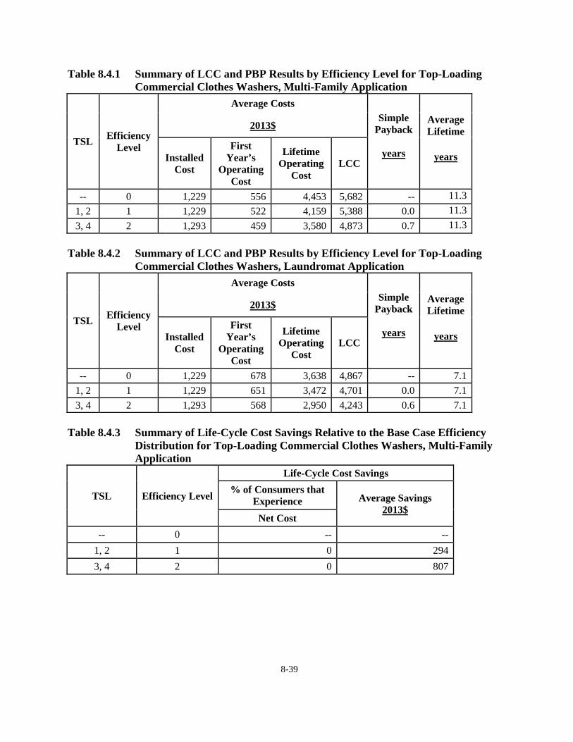
Table 8.4.1 Summary of LCC and PBP Results by Efficiency Level for Top-Loading Commercial Clothes Washers, Multi-Family Application
TSL Efficiency Level
Average Costs Simple
Payback
years
2013$ Average Lifetime
Installed Cost
First Year’s
Operating Cost
Lifetime Operating
Cost LCC
years
-- 0 1,229 556 4,453 5,682 -- 11.3 1, 2 1 1,229 522 4,159 5,388 0.0 11.3 3, 4 2 1,293 459 3,580 4,873 0.7 11.3
Table 8.4.2 Summary of LCC and PBP Results by Efficiency Level for Top-Loading
Commercial Clothes Washers, Laundromat Application
TSL Efficiency Level
Average Costs Simple
Payback
years
2013$ Average Lifetime
Installed Cost
First Year’s
Operating Cost
Lifetime Operating
Cost LCC
years
-- 0 1,229 678 3,638 4,867 -- 7.1 1, 2 1 1,229 651 3,472 4,701 0.0 7.1 3, 4 2 1,293 568 2,950 4,243 0.6 7.1
Table 8.4.3 Summary of Life-Cycle Cost Savings Relative to the Base Case Efficiency
Distribution for Top-Loading Commercial Clothes Washers, Multi-Family Application
TSL Efficiency Level
Life-Cycle Cost Savings % of Consumers that
Experience Average Savings 2013$
Net Cost -- 0 -- --
1, 2 1 0 294 3, 4 2 0 807
8-39

Table 8.4.4 Summary of Life-Cycle Cost Savings Relative to the Base Case Efficiency Distribution for Top-Loading Commercial Clothes Washers, Laundromat Application
TSL Efficiency Level
Life-Cycle Cost Savings
% of Consumers that Experience Average Savings
2013$ Net Cost
-- 0 -- -- 1, 2 1 0 166 3, 4 2 0 622
Table 8.4.5 Summary of LCC and PBP Results by Efficiency Level for Front-Loading
Commercial Clothes Washers, Multi-Family Application
TSL Efficiency Level
Average Costs Simple
Payback
years
2013$ Average Lifetime
Installed Cost
First Year’s
Operating Cost
Lifetime Operating
Cost LCC
years
-- 0 1,817 409 2,915 4,732 -- 11.3 1 1 1,817 384 2,695 4,512 0.0 11.3
2, 3 2 1,818 364 2,519 4,337 0.0 11.3 4 3 1,848 381 2,659 4,507 1.1 11.3
Table 8.4.6 Summary of LCC and PBP Results by Efficiency Level for Front-Loading
Commercial Clothes Washers, Laundromat Application
TSL Efficiency Level
Average Costs Simple
Payback
years
2013$ Average Lifetime
Installed Cost
First Year’s
Operating Cost
Lifetime Operating
Cost LCC
years
-- 0 1,817 524 2,452 4,269 -- 7.1 1 1 1,817 493 2,266 4,082 0.0 7.1
2, 3 2 1,818 471 2,133 3,951 0.0 7.1 4 3 1,848 491 2,243 4,092 1.0 7.1
8-40

Table 8.4.7 Summary of Life-Cycle Cost Savings Relative to the Base Case Efficiency Distribution for Front-Loading Commercial Clothes Washers, Multi-Family Application
TSL Efficiency Level
Life-Cycle Cost Savings % of Consumers that
Experience Average Savings 2013$
Net Cost -- 0 -- -- 1 1 0 221
2, 3 2 0 272 4 3 55 -3
Table 8.4.8 Summary of Life-Cycle Cost Savings Relative to the Base Case Efficiency
Distribution for Front-Loading Commercial Clothes Washers, Laundromat Application
TSL Efficiency Level
Life-Cycle Cost Savings % of Consumers that
Experience Average Savings 2013$
Net Cost -- 0 -- -- 1 1 0 184
2, 3 2 0 212 4 3 65 -10 Figure 8.4.6 and Figure 8.4.7 show the range of LCC savings for the efficiency levels for
both product applications of top-loading commercial clothes washers. Figure 8.4.8 and Figure 8.4.9 show the range of LCC savings for the efficiency levels for both product applications of front-loading commercial clothes washers. For each EL, the top and the bottom of the box indicate the 75th and 25th percentiles, respectively. The bar at the middle of the box indicates the median; 50 percent of the households have LCC savings above this value The ‘whiskers’ at the bottom and the top of the box indicate the 5th and 95th percentiles. The small box shows the average LCC savings for each EL.
8-41

Figure 8.4.6 Range of LCC Savings for Top-Loading Commercial
Clothes Washers, Multi-Family
Figure 8.4.7 Range of LCC Savings for Top-Loading Commercial
Clothes Washers, Laundromat
0
200
400
600
800
1,000
1,200
1,400
1,600
Level 1 Level 2
Life
Cyc
le Co
st Sa
ving
s ($)
Efficiency Level
median average
0
200
400
600
800
1,000
1,200
Level 1 Level 2
Life
Cyc
le C
ost S
avin
gs ($
)
Efficiency Level
median average
8-42
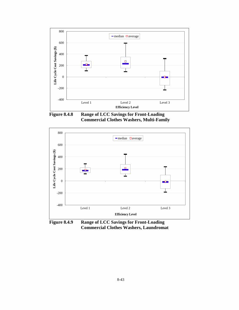
Figure 8.4.8 Range of LCC Savings for Front-Loading
Commercial Clothes Washers, Multi-Family
Figure 8.4.9 Range of LCC Savings for Front-Loading
Commercial Clothes Washers, Laundromat
-400
-200
0
200
400
600
800
Level 1 Level 2 Level 3
Life
Cyc
le C
ost S
avin
gs ($
)
Efficiency Level
median average
-400
-200
0
200
400
600
800
Level 1 Level 2 Level 3
Lif
e C
ycle
Cos
t Sav
ings
($)
Efficiency Level
median average
8-43

8.5 REBUTTABLE PAYBACK PERIOD
DOE presents rebuttable PBPs to provide the legally established rebuttable presumption that an energy efficiency standard is economically justified if the additional product costs attributed to the standard are less than three times the value of the first-year energy cost savings. (42 U.S.C. §6295 (o)(2)(B)(iii))
8.5.1 Metric
The basic equation for rebuttable PBP is the same as that shown in section 8.3, Payback Period Inputs. Unlike the analyses described in sections 8.2 and 8.3, however, the rebuttable PBP is not based on the use of household samples and probability distributions. Rather than distributions, the rebuttable PBP is based on discrete single-point values. For example, while DOE uses a probability distribution of regional energy prices in the distributional payback period analysis, it uses only the national average energy price from the probability distribution to determine the rebuttable PBP. Other than the use of single-point values, the most notable difference between the distribution PBP and the rebuttable PBP is the latter’s reliance on the DOE test procedure to determine a product’s annual energy and water consumption. The following identifies the differences between the annual energy and water consumptions determined for the distribution PBP and the rebuttable PBP. DOE based the annual energy and water consumption values that it used to determine the rebuttable PBP on the number of cycles per year specified in the DOE test procedure.25 The commercial clothes washer test procedure cites the residential clothes washer test procedure to establish efficiency ratings as well as annual energy and water consumption. As a result, the annual number of use cycles, 295 cycles per year, for determining the annual energy and water consumption of commercial clothes washers is representative of residential use, not commercial use. Because residential use is significantly lower than the average usage for commercial applications—1460 cycles per year in multi-family buildings and 2190 cycles per year in laundromats—the average annual energy and water consumption used to determine rebuttable PBP will be significantly less than the consumption associated with actual usage. As a result, the rebuttable PBP will be significantly longer than the distribution PBPs for both multi-family and laundromat applications.
8.5.2 Inputs
Inputs for the rebuttable PBP differ from the distribution PBP in that the calculation uses discrete values, rather than distributions, for inputs. Note that for the calculation of distribution PBP, because inputs for the determination of total installed cost were based on single-point values, only the variability and/or uncertainty in the inputs for determining operating cost contributed to variability in the distribution PBPs. The following summarizes the single-point values that DOE used in the determination of the rebuttable PBP.
8-44

• Manufacturing costs, markups, sales taxes, and installation costs were all based on the single-point values used in the distributional LCC and PBP analysis.
• As described in section 8.5.1, annual energy and water consumption is based on the DOE
test procedure.
• Energy and water prices are based on national average values for the year that new standards are assumed to take effect.
• An average discount rate or lifetime is not required in the rebuttable PBP calculation.
• The effective date of the standard is assumed to be 2018.
8.5.3 Results
DOE calculated rebuttable PBPs for each efficiency level relative to the distribution of product efficiencies assumed for the base case (refer back to section 8.2.6 for more details on the base case efficiency distributions for each product). In other words, DOE did not determine the rebuttable PBP relative to the baseline efficiency level, but relative to the current distribution of product efficiencies DOE determined for the base case (i.e., the case without new standards). The following sections present the results for the sets of products being analyzed for this standards rulemaking. Table 8.5.1 and Table 8.5.2 present the rebuttable PBPs for top-loading commercial clothes washers under both product applications; multi-family buildings and laundromats. Table 8.5.3 and Table 8.5.4 present the rebuttable PBPs for front-loading commercial clothes washers under both product applications; multi-family buildings and laundromats. Table 8.5.1 Top-Loading Commercial Clothes Washers, Multi-Family Application:
Rebuttable Payback Periods
Efficiency Level MEF IWF PBP years
Baseline 1.15 8.90 - 1 1.35 8.80 0 2 1.55 6.90 2.6
8-45

Table 8.5.2 Top-Loading Commercial Clothes Washers, Laundromat Application: Rebuttable Payback Periods
Efficiency Level MEF IWF PBP years
Baseline 1.15 8.90 - 1 1.35 8.80 0 2 1.55 6.90 3.1
Table 8.5.3 Front-Loading Commercial Clothes Washers, Multi-Family Application:
Rebuttable Payback Periods
Efficiency Level MEF IWF PBP years
Baseline 1.65 5.20 - 1 1.80 4.50 0 2 2.00 4.10 0.1 3 2.20 3.90 11.2
Table 8.5.4 Front-Loading Commercial Clothes Washers, Laundromat Application:
Rebuttable Payback Periods
Efficiency Level MEF IWF PBP years
Baseline 1.65 5.20 - 1 1.80 4.50 0 2 2.00 4.10 0.1 3 2.20 3.90 11.1
8-46

REFERENCES
1 RS Means Company Inc., RS Means Mechanical Cost Data, 36st Annual Edition. 2013. Kingston, MA.
2 U.S. Department of Energy–Energy Information Administration, Form EIA-861 for
2012, 2013. (Last accessed November, 2013.) http://www.eia.gov/electricity/data/eia861 3 U.S. Census Bureau, Population Estimates, National Totals: Vintage 2013, (Last
accessed November, 2013.) < http://www.census.gov/popest/data/national/totals/2013/index.html>
4 U.S. Department of Energy-Energy Information Administration, Natural Gas Prices,
2013. Washington, DC. http://www.eia.gov/dnav/ng/ng_pri_sum_dcu_nus_m.htm
5 Raftelis Financial Consultants Inc., 2012 RFC/AWWA Water and Wastewater Rate
Survey, 2013. Charlotte, NC, Kansas City, MO, and Pasadena, CA. http://www.raftelis.com/news/rfcawwa-2012-water-and-wastewater-rate-survey-now-available/
6 U.S. Department of Energy-Energy Information Administration, Annual Energy Outlook
2014 with Projections to 2040, 2014. Washington, DC. http://www.eia.gov/forecasts/aeo/ 7 U.S. Department of Labor-Bureau of Labor Statistics, Consumer Price Indexes, Item:
Water and sewerage maintenance, Series Id: CUUR0000SEHG01, U.S. city average (not seasonally adjusted), 2013. Washington, DC. http://www.bls.gov/cpi/
8 Whirlpool Corporation, Comment of Whirlpool Corporation Regarding the ANOPR for
Cooking Products and Commercial Clothes Washers. 9 U.S. Department of Energy-Energy Efficiency and Renewable Energy, Technical
Support Document: Energy Efficiency Standards for Consumer Products: Residential Central Air Conditioners and Heat Pumps Including: Regulatory Impact Analysis. Chapter 5, Life-Cycle Cost and Payback Analysis, May, 2002. Washington, D.C. http://www1.eere.energy.gov/buildings/appliance_standards/residential/ac_central_1000_r.html
10 Coin Laundry Association, Industry Overview. Downers Grove, IL.
http://www.coinlaundry.org/investor-resources/industry-overview 11 Southern California Edison, 2004-2005 Database for Energy Efficiency Resources
(DEER) Update Study, Final Report, December, 2005. Prepared for Southern California Edison by Itron, Inc. Vavcouver, WA. http://www.calmac.org/publications/2004-05_DEER_Update_Final_Report-Wo.pdf
8-47

12 Sullivan, G. P., J. W. Currie, T. C. Hillman, and G. B. Parker, High-Performance Clothes Washer Demonstration at Leisure World Laguna Woods Final Report, December, 2000. Prepared for Southern California Edison Company by Battelle Pacific Northwest Laboratory. Richland, WA. http://eere.pnl.gov/building-technologies/doc/scefinal%202-22-01.pdf
13 California Measurement Advisory Committee, CALMAC Protocols, Appendix F,
Effective Useful Live Values for Major Energy Efficiency Measures, September, 2000. http://www.calmac.org/events/APX_F.pdf
14 Modigliani, F. and M. Miller, The Cost of Capital, Corporation Finance and the Theory of
Investment. American Economic Review, 1958. June: pp. 261-297 . 15 Damodaran Online, The Data Page: Cost of Capital by Industry Sector, 2001-2013. (Last
accessed March, 2014.) http://pages.stern.nyu.edu/~adamodar/
16 Ibbotson Associates, Cost of Capital 2009 Yearbook. 2009. Ibbotson Associates:
Chicago, IL. 17 The Federal Reserve Board, Federal Reserve Statistical Release, Selected Interest Rates,
Historical Data, Instrument: State and local bonds, Maturity: 20-year, Frequency: Monthly, Description: Bond buyer go 20-bond municipal bond index, 2013. www.federalreserve.gov/releases/H15/data.htm
18 U.S. Energy Information Agency, Commercial Buildings Energy Consumption Survey,
1992. (Last accessed August, 2013.) http://www.eia.gov/consumption/commercial/data/1992/index.cfm?view=microdata
19 Federal Reserve Board, Federal Reserve Bank Services Private Sector Adjustment Factor,
2005, 2005. Washington, D.C. http://www.federalreserve.gov/boarddocs/Press/other/2005/20051012/attachment.pdf
20 U.S. Energy Information Agency, Commercial Buildings Energy Consumption Survey,
1995. (Last accessed August, 2013.) http://www.eia.gov/consumption/commercial/data/1995/index.cfm?view=microdata
21 Damodaran Online Data Page, The Data Page: Historical Returns on Stocks, Bonds and
Bills - United States, 2013. Damodaran. (Last accessed June, 2014.) http://pages.stern.nyu.edu/~adamodar/
22 Association of Home Appliance Manufacturers (AHAM), AHAM Data on Commercial
Clothes Washers for DOE Efficiency Standards Rulemaking, August 11, 2014. 2014, Letter to Building Technologies Program, U.S. Department of Energy.
8-48

23 DOE Compliance Certification Database for Commercial Clothes Washers, 2014.
<http://www.regulations.doe.gov/certification-data/CCMS-79222370561.html> 24 ENERGY STAR, Commercial Clothes Washers.
<http://www.energystar.gov/products/certified-products/detail/commercial-clothes-washers>
25 U.S. Office of the Federal Register, Code of Federal Regulations, Title 10, Part 431 -
Energy Conservation Program for Certain Commercial and Industrial Equipment, Subpart I—Commercial Clothes Washers, January 1, 2007. Washington, DC.
8-49