Chapter 8 Julia Tutorial - sas.upenn.edujesusfv/Chapter_HPC_8_Julia.pdf · Other members of the...
55
Chapter 8 Julia Tutorial 8.1 Why Julia? Julia is a modern, expressive, high-performance programming language designed for sci- entific computation and data manipulation. Originally developed by a group of computer scientists and mathematicians at MIT, Julia combines three key features for highly inten- sive computing tasks as perhaps no other contemporary programming language does: it is fast, easy to learn and use, and open source. Among its competitors, C/C++ is extremely fast and the open-source compilers available for it are excellent, but it is hard to learn, in particular for those with little programming experience, and cumbersome to use, for example when prototyping new code. 1 Python and R are open source and easy to learn and use, but their numerical performance can be disappointing. 2 Matlab is relatively fast (although quite less than Julia) and it is easy to learn and use, but it is rather costly to purchase and its age is starting to show. 3 Julia delivers its swift numerical speed thanks to the reliance on a LLVM (Low Level Virtual Machine)-based JIT (just-in-time) compiler. As a beginner, you do not have to be concerned much about what this means except to realize that you do not need to “compile” Julia in the way you compile other languages to achieve lightning-fast speed. Thus, you avoid an extra layer of complexity (and, often, maddening frustration while dealing with obscure compilation errors). 1 Although technically two different languages, C and C++ are sufficiently close that we can discuss them together for this chapter. Other members of the “curly-bracket” family of programming languages (C#, Java, Swift, Kotlin,...) face similar problems and are, for a variety of reasons, less suitable for numerical computations. 2 Using tools such as Cython, Numba, or Rcpp, these two languages can be accelerated. But, ultimately, these tools end up creating bottlenecks (for instance, if you want to have general user-defined types or operate with libraries) and limiting the scope of the language. These problems are especially salient in large projects. 3 GNU Octave and Scilab are open-source near-clones of Matlab, but their execution speed is generally poor. 57
Transcript of Chapter 8 Julia Tutorial - sas.upenn.edujesusfv/Chapter_HPC_8_Julia.pdf · Other members of the...

Chapter 8
Julia Tutorial
8.1 Why Julia?
Julia is a modern, expressive, high-performance programming language designed for sci-
entific computation and data manipulation. Originally developed by a group of computer
scientists and mathematicians at MIT, Julia combines three key features for highly inten-
sive computing tasks as perhaps no other contemporary programming language does: it is
fast, easy to learn and use, and open source. Among its competitors, C/C++ is extremely
fast and the open-source compilers available for it are excellent, but it is hard to learn, in
particular for those with little programming experience, and cumbersome to use, for example
when prototyping new code.1 Python and R are open source and easy to learn and use, but
their numerical performance can be disappointing.2 Matlab is relatively fast (although quite
less than Julia) and it is easy to learn and use, but it is rather costly to purchase and its
age is starting to show.3 Julia delivers its swift numerical speed thanks to the reliance on
a LLVM (Low Level Virtual Machine)-based JIT (just-in-time) compiler. As a beginner, you
do not have to be concerned much about what this means except to realize that you do not
need to “compile” Julia in the way you compile other languages to achieve lightning-fast
speed. Thus, you avoid an extra layer of complexity (and, often, maddening frustration while
dealing with obscure compilation errors).
1Although technically two different languages, C and C++ are sufficiently close that we can discuss themtogether for this chapter. Other members of the “curly-bracket” family of programming languages (C#,Java, Swift, Kotlin,...) face similar problems and are, for a variety of reasons, less suitable for numericalcomputations.
2Using tools such as Cython, Numba, or Rcpp, these two languages can be accelerated. But, ultimately,these tools end up creating bottlenecks (for instance, if you want to have general user-defined types or operatewith libraries) and limiting the scope of the language. These problems are especially salient in large projects.
3GNU Octave and Scilab are open-source near-clones of Matlab, but their execution speed is generallypoor.
57

58 CHAPTER 8. JULIA TUTORIAL
Furthermore, Julia incorporates in its design important advances in programming lan-
guages –such as a superb support for parallelization or practical functional programming
orientation– that were not fully fleshed out when other languages for scientific computation
were developed a few decades ago. Among other advances that we will discuss in the follow-
ing pages, we can highlight multiple dispatching (i.e., functions are evaluated with different
methods depending on the type of the operand), metaprogramming through Lisp-like macros
(i.e., a program that transforms itself into new code or functions that can generate other
functions), and the easy interoperability with other programming languages (i.e., the ability
to call functions and libraries from other languages such as C++ and Python). These advances
make Julia a general-purpose language capable of handling tasks that extend beyond scien-
tific computation and data manipulation (although we will not discuss this class of problems
in this tutorial).
Finally, a vibrant community of Julia users is contributing a large number of packages
(a package adds additional functionality to the base language; as of December 14, 2017, there
are 1686 registered packages). While Julia’s ecosystem is not as mature as C++, Python
or R’s, the growth rate of the penetration of the language is increasing. In the well-known
TIOBE Programming Community Index for January 2018, Julia appears in position 47,
close to venerable languages such as Logo and Lisp and at a striking distance of Fortran.
The next sections introduce elementary concepts in Julia. They assume some familiarity
with how to interact with scripting programming languages such as Python, R, Matlab, or
Stata and a basic knowledge of programming structures (loops and conditionals). The tuto-
rial is not, however, a substitute for a whole manual on Julia or the online documentation.4
If you have coded with Matlab for a while, you must resist the temptation of thinking that
Julia is a faster Matlab. It is true that Julia’s basic syntax (definition of vectors and matri-
ces, conditionals, and loops) is, by design, extremely close to Matlab’s. This similarity allows
Matlab’s users to start coding in Julia nearly right away. But, you should try to make an
effort to understand how Julia allows you to do many new things and to re-code old things in
more elegant and powerful ways than in Matlab. Pay close attention, for instance, to the fact
that Julia (quite sensibly) passes arguments by reference and not by value as Matlab or to
our description of currying and closures. Those readers experienced with compiled languages
such as C++ or Fortran will find that most of the material presented here is trivial, but they
nevertheless may learn a thing or two about the awesome features of Julia.
4Among recent books on Julia, you can check Balbaert, Sengupta, and Sherrington (2016) (whichcollates three previous books published by the authors) and Nagar (2017). The official documentationcan be found at https://docs.julialang.org/en/stable/index.html. See also the Quantitative Eco-nomics webpage at https://lectures.quantecon.org/jl/ for applications of Julia in economics andhttps://www.juliabloggers.com/ for an aggregator of blogs about Julia.

8.2. INSTALLING JULIA 59
8.2 Installing Julia
The best way to get all the capabilities from the language in a convenient environment is
to install JuliaPro from Julia Computing.5 The Personal version is free and comes with
extra material, including a profiler and more than 100 packages (other versions and products
from the company are available for a charge, but most likely you will not need them). The
webpage of the company provides with more detailed installation instructions for your OS
and the different ways in which you can interact with Julia.
Figure 8.1: JuliaPro
Once you have installed JuliaPro, you can open it by clicking in its icon. Technically,
JuliaPro lunches Juno, an IDE based on the atom editor. Figure 8.1 reproduces a screenshot
of JuliaPro on a Mac computer with the atom Dark user interface (UI) theme and the
Cobalt2 syntax theme (you can configure the user interface and syntax with hundreds of
existing color themes available for atom or even to design your own!).
5See https://juliacomputing.com/. Julia Computing is the company created by the original Juliadevelopers and two partners to monetize their research through the provision of extra services and technicalsupport. Julia itself is open source.

60 CHAPTER 8. JULIA TUTORIAL
In Figure 8.1, the console tab for commands with a prompt appears at the bottom center
of the window (the default), although you can move it to any position is convenient for you
(the same applies to all the other tabs of the IDE). This console implements a REPL: you
type a command, you enter return, and you see the result on the screen. REPL, pronounced
“repple,” stands for Read–Eval–Print Loop and it is just an interactive shell like the one you
might have seen in other programming languages.6 Thus, the console will be the perfect way
to test on your own the different commands and keywords that we will introduce in the next
pages and see the output they generate. For example, a first command you can learn is:
versioninfo() # version information
This command will tell you the version you have installed of Julia and its libraries and some
details about your computer and OS. Note that any text after the hashtag character # is a
comment and you can skip it:
# This is a comment
Below, we will write comments after the commands to help you read the code boxes.
As you start typing, you will note that JuliaPro has autocompletion: before you finish
typing a command, the REPL console or the editor will suggest completions. You will soon
realize that the number of suggestions is often large, a product of the richness of the language.
A space keystroke will allow you to eliminate the suggestions and continue with the regular
use of the console.
Julia will provide you with more information on a command or function if you type ?
followed by the name of the command or function.
? cos # info on function cos
The explanations in the help function are usually clear and informative and many times come
with a simple example of how to apply the command or function in question.
You can also navigate the history of REPL commands with the up and down arrow keys,
suppress the output with ; after the command (in that way, you can accumulate several
commands in the same line), and activate the shell of your OS by typing ; after the prompt
without any other command (then, for example, if you are a Unix user you can employ
directory navigation commands such as pwd , ls , and so on and pipelining). Finally, you
can clear the console either with a button at the top of the console or with the command
clearconsole() . The next box summarizes these commands:
6The REPL comes with several key bindings for standard operations (copy, paste, delete, etc.) and searches,but if you are using JuliaPro, you have buttons and menus to accomplish the same goals without memo-rization.

8.2. INSTALLING JULIA 61
? cos # info on function cos
up arrow key # previous command
down arrow key # next command
3+2; # ; suppresses output if working on the REPL
; # activates shell model
clearconsole() # clearconsole
The result from the last computation performed by Julia will always be stored in ans :
ans # previous answer
You can use ans as any other variable or even redefine it:
ans+1.0 # adds 1.0 to the previous answer
ans = 3.0 # makes ans equal to 3.0
println(ans) # prints ans in screen
If there was no previous computation, the value of ans will be nothing . Also, JuliaPro
will present the results of a computation in compact form (i.e., like 1.00e+3 ). Click on it
to get the full format (i.e., 1000.0 ).
Other parts of the IDE include an editor tab, to write longer blocks of code and save it
as files (you can keep multiple files opened simultaneously), a workspace tab, where values of
variables and functions will be displayed, a plots tab, for graphic visualization, and a toolbar
at the left to control Julia. As options, you can add Git and Github tabs to implement
version control, a tree view of your project tab (i.e., the structure of the directory with the
files in a software project), and a command palette tab.
However, before proceeding further, you want to type in the console tab:
Pkg.init()
Pkg.update()
Pkg.add("IJulia")
The first command, Pkg.init() , will initialize a package repository for your Julia’s
installation. The second command, Pkg.update() , will update all existing packages (this
is redundant after an initialization of a package repository, but a good check that everything
went well so far). The third command, Pkg.add("IJulia") , will add the package IJulia
that we will need below. Be patient: each command might take some time to complete, but
this only needs to be done when you first install JuliaPro. In Section 8.3, we will discuss
in more detail what a package is and how to install and maintain them, but these three
commands will suffice for the moment.

62 CHAPTER 8. JULIA TUTORIAL
There are other two ways to use JuliaPro. One is to lunch a terminal window in the OS
with the command Julia>Open Terminal that you can find in the top menu of JuliaPro.7
You can see a screenshot of such a REPL terminal in Figure 8.2 with a prompt to type a
command (the color theme of your console can be different than the one shown here). If
you install Julia directly from https://julialang.org/downloads/, you will have access
to this same command-line terminal, but not to the rest of JuliaPro.8
Figure 8.2: Julia terminal process
Finally, JuliaPro allows you to open IJulia, a graphical notebook interface with the
popular Project Jupyter that we introduced in Chapter 7 (recall that to run IJulia, you
need first to install the package IJulia ). In the REPL –either the console of JuliaPro or
a Julia terminal window,– you type:
using IJulia
notebook()
and a notebook will open in your default browser. The notebook will be connected with the
Julia’s kernel (lunched by the command IJulia ) and allow you to run the same commands
7If you find the path where JuliaPro installed Julia in your computer, you can call it directly from aterminal window of your OS or create a shortcut to do so.
8Unless you have more experience with computers, you do not want to have two simultaneous installa-tions of Julia, one from JuliaPro and one from https://julialang.org/downloads/, as this may createcompatibility problems.
8.2. INSTALLING JULIA 63
that the regular REPL.
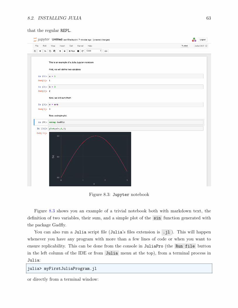
Figure 8.3: Jupyter notebook
Figure 8.3 shows you an example of a trivial notebook both with markdown text, the
definition of two variables, their sum, and a simple plot of the sin function generated with
the package Gadfly.
You can also run a Julia script file (Julia’s files extension is .jl ). This will happen
whenever you have any program with more than a few lines of code or when you want to
ensure replicability. This can be done from the console in JuliaPro (the Run file button
in the left column of the IDE or from Julia menu at the top), from a terminal process in
Julia:
julia> myFirstJuliaProgram.jl
or directly from a terminal window:
64 CHAPTER 8. JULIA TUTORIAL
$ julia myFirstJuliaProgram.jl
For this last option, though, you need to either work from the directory where Julia is
installed or configure your Path accordingly.
There are alternative ways to run Julia. For example, it can be bound to a large class of
editors and IDEs such as Emacs, Subversive, Eclipse, and many others. However, unless
you have a strong reason (i.e., long experience with one of the other tools, the need to integrate
with a larger team or project, multilanguage programming), our advice will be to stick with
JuliaPro.
8.3 Packages
As we explained in Section 8.1, a package is code that extends the basic capabilities Julia
with additional functions, data structures, etc. In such a way, Julia follows the modern
trend of open source software of having a base installation of a project and a lively ecosystem
of developers creating specialized tools that you can add or remove at will. LATEX, R, and
Atom, for example, work in a similar way.
We also saw in Section 8.2, that one of the first things you may want to do after installing
Julia is to initialize the package repository, Pkg.init() , and update all the packages that
come with the basic installation of JuliaPro, Pkg.update() . Julia comes with a built-in
package manager linked with a repository in GitHub called METaDaTa that will take care of
issues such as updating dependencies.
Other useful commands related with package management include:
Pkg.status()
Pkg.installed()
Pkg.add("Gadfly")
Pkg.rm("Gadfly")
Pkg.status() prints the status of all installed packages. Pkg.installed() accomplishes
the same task than the previous command, except that it returns a dictionary (an associative
array; we will explain below what dictionaries are and how to use them). Pkg.add("Gadfly")
checks whether the package Gadfly is already installed and, if not, installs it. This plotting
package will allow you to prepare beautiful plots.9 If Gadfly is already added (this will be
the case if you installed JuliaPro), you will get a message:
9You can check http://gadflyjl.org/stable/. Gadfly follows Hadley Wickhams’s ggplot2 for R andthe ideas of Wilkinson (2005).

8.3. PACKAGES 65
INFO: Package Gadfly is already installed
and you do not need to do anything else. Pkg.rm("Gadfly") will remove the package, but
hopefully you will be convinced that Gadfly is a good package to keep.
The same commands work if you substitute Gadfly for the name of any package. All
registered packages are listed at https://pkg.julialang.org/, but there are additional
unregistered ones that you can find on the internet or from colleagues. Finally, you might
want to run Pkg.update() periodically to update your packages.
The general command to use a package in your code or in the console is
using Gadfly
If, instead, you only want to use a function from a package (for instance, to avoid some
conflicts among functions from different packages or to get around some instability in a
package), you can use
import Gadfly: plot
In most occasions, however, importing the whole package will be the simplest approach and
the recommended default.
Other useful packages in economics are:
1. QuantEcon : Quantitative Economics functions for Julia.
2. Plots : easy plots.
3. PyPlot : plotting for Julia based on matplotlib.pyplot.
4. Distributions : probability distributions and associated functions.
5. DataFrames : to work with tabular data.
6. Pandas : a front-end to work with Python’s Pandas.
7. TensorFlow : a Julia wrapper for TensorFlow.
Several packages facilitate the interaction of Julia with other common programming
languages. Among those, we can highlight:
1. Pycall : call Python functions.
2. JavaCall : call Java from Julia.
66 CHAPTER 8. JULIA TUTORIAL
3. RCall : embedded R within Julia.
Recall, also, that Julia can directly call C++ and Python’s functions. And note that most of
these packages come already with the JuliaPro distribution.
There are additional commands to develop and distribute packages, but that material is
too advanced for an introductory tutorial.
8.4 Types
Julia has variables, values, and types. A variable is a name bound to a value. Julia is case
sensitive: a is a different variable than A . In fact, as we will see below, the variable can
be nearly any combination of Unicode characters. A value is a content (1, 3.2, ”economics”,
etc.). Technically, Julia considers that all values are objects (an object is an entity with
some attributes). This makes Julia closer to pure object-oriented languages such as Ruby
than to languages such as C++, where some values such as floating points are not objects.
Finally, values have types (i.e., integer, float, boolean, string, etc.). A variable does not have
a type, its value has. Types specify the attributes of the content. Functions in Julia will
look at the type of the values passed as operands and decide, according to them, how we
can operate on the values (i.e., which of the methods available to the function to apply).
Adding 1+2 (two integers) will be different than summing 1.0+2.0 (two floats) because the
method for summing two integers is different from the method to sum two floats. In the base
implementation of Julia, there are 181 different methods for the function sum! You can list
them with the command methods() as in:
methods(+) # methods for sum
This application of different methods to a common function is known as polymorphic multiple
dispatch and it is one of the key concepts in Julia you need to understand.10
The previous paragraph may help to see why Julia is a strongly dynamically typed
programming language. Being a typed language means that the type of each value must be
known by the compiler at run time to decide which method to apply to that value. Being a
dynamically typed language means that such knowledge can be either explicit (i.e., declared
by the user) or implicit (i.e., deduced by Julia with an intelligent type inference engine from
the context it is used). Dynamic typing makes developing code with Julia flexible and fast:
10Multiple dispatch is different from the overloading of operators existing in languages such as C++ becauseit is determined at run time, not compilation time. Later, when we introduce composite types, we will see asecond difference: in Julia methods are not defined within classes as you would do in most object-orientedlanguages.
8.4. TYPES 67
you do not need to worry about explicitly type every value as you go along (i.e., declaring to
which type the value belongs to). Being a strongly typed language means that you cannot
use a value of one type as another value, although you can convert it or let the compiler do it
for you. For example, Julia follows a promotion system where values of different types being
operated jointly are “promoted” to a common system: in the sum between an integer and a
float, the integer is “promoted” to float.11 You can, nevertheless, impose that the compiler
will not vary the type of a value to avoid subtle bugs in issues where the type is of critical
importance such as array indexing and, sometimes, to improve performance by providing
guidance to the JIT compiler on which methods to implement.
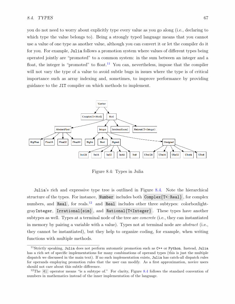
Figure 8.4: Types in Julia
Julia’s rich and expressive type tree is outlined in Figure 8.4. Note the hierarchical
structure of the types. For instance, Number includes both Complex{T<:Real} , for complex
numbers, and Real , for reals.12 and Real includes other three subtypes: colorboxlight-
grayInteger, Irrational{sim} , and Rational{T<Integer} . These types have another
subtypes as well. Types at a terminal node of the tree are concrete (i.e., they can instantiated
in memory by pairing a variable with a value). Types not at terminal node are abstract (i.e.,
they cannot be instantiated), but they help to organize coding, for example, when writing
functions with multiple methods.
11Strictly speaking, Julia does not perform automatic promotion such as C++ or Python. Instead, Juliahas a rich set of specific implementations for many combinations of operand types (this is just the multipledispatch we discussed in the main text). If no such implementation exists, Julia has catch-all dispatch rulesfor operands employing promotion rules that the user can modify. As a first approximation, novice usersshould not care about this subtle difference.
12The <: operator means “is a subtype of.” For clarity, Figure 8.4 follows the standard convention ofnumbers in mathematics instead of the inner implementation of the language.
68 CHAPTER 8. JULIA TUTORIAL
You do not need, though, to remember the type tree hierarchy, since Julia provides you
with commands to check the supertype (i.e., the type above a current type in the tree) and
subtype (i.e., the types below) of any given type:
supertype(Float64) # supertype of Float64
subtypes(Integer) # subtypes of Integer
This type tree can integrate and handle user-defined types (i.e., types with properties
defined by the programmer) as fast and compactly as built-in types. In Julia, this user-
defined types are called composite types. A composite type is the equivalent in Julia to
structs and objects in C/C++, Python, Matlab, and R, although they do not incorporate
methods, functions do. If these two last sentencess look obscure to you: do not worry! You
are not missing anything of importance right now. We will delay a more detailed discussion
of composite types until Section 8.8 and then you will be able to follow the argument much
better.
You can always check the type of a variable with
typeof(a) # type of a
Later, when we learn about iterated collections, you might find useful to check their type
with:
# determine type of elements in collection a
eltype(a)
You can fix the type a variable with the operator :: (read as “is an instance of”):
a::Float64 # fixes type of a to generate type-stable code
b::Int = 10 # fixes type and assigns a value
You can also check the memory address of a value
a = 1
pointer_from_objref(a)
which will return something that looks like PtrVoid @0x000000010f23c090 and its size in
memory:
sizeof(a)
which will return 8 (integers use little memory!).13
13If you are a C/C++ programer, do not use this pointer in the way your instinct will tell you to do it. Aswe will see later, Julia passes arguments by reference, a simpler way to manage memory.

8.4. TYPES 69
If you want to know more about the state of your memory at any given time, you can
check the workspace in JuliaPro or type
whos()
In comparision with Matlab, Julia does not have a command to clear the workspace. You
can always liberate memory by equating a large object to zero:
a = 0
or by running the garbage collector
gc() # garbage collector
Be careful though! Only run the garbage collector if you understand what a garbage collector
is. Chances are you will never need to do so.
Julia’s sophisticated type structure provides you with extraordinary capabilities. For
instance, you can use a greek letter as a variable by typing its LATEX’s name plus pressing
tab:
\alpha (+ press Tab)
This α is a variable that can operated upon like any other regular variable in Julia, i.e.,
we can sum to another variable, divide it, etc. This is particularly useful when coding
mathematical functions with parameters expressed in terms of greek letters, as we usually do
in economics. The code will be much easier to read and maintain.
You can extend this capability of to all Unicode characters and operate on exotic vari-
ables:14
# Create a variable called aleph with value 3
\aleph (+ press Tab) = 3
# Creates a whale with value 2
\:whale: (+ press Tab) = 2
# Sum both
\aleph (+ press Tab) + \:whale: (+ press Tab)
In addition, and quite unique among programming languages, Julia has an irrational
type, with variables such as π = 3.1415... or e = 2.7182... already predefined
14Unicode is an industry standard maintained by the Unicode Consortium (http://www.unicode.org/.In its latest June 2017 release, it includes 136,755 characters, including 139 modern and historic scripts. Ifyou need to perform, for example, an statistical analysis of a text written in Imperial aramaic, Julia is yourperfect choice.
70 CHAPTER 8. JULIA TUTORIAL
pi (+ press Tab) # returns 3.14...
e (+ press Tab) # returns 2.72...
typeof(pi (+ press Tab))
and rational type on which you can perform standard fraction operations:
a = 1 // 2 # note // operator instead of /
b = 3//7
c = a+b
numerator(c) # finds numerator of c
denominator(c) # finds denominator of c
Julia will reduce a rational if the numerator and denominator have common factors.
a = 15 // 9
returns a = 5 // 3 .
Infinite rational numbers are acceptable:
a = 1 // 0
but a NaN is not:
a = 0 // 0 # this will generate an error message
If you want to transform a rational back into a float, you only need to write:
float(c)
and to create a rational from a float:
# approximate representation of the float, the return that you expect
rationalize(1.20)
# exact representation of the float, perhaps not the return that you expect
Rational(1.20)
The presence of irrational and rational types show the strong numerical orientation of the
language.
8.5. FUNDAMENTAL COMMANDS 71
8.5 Fundamental commands
We enter now into four sections that constitute the core of the tutorial. In this section,
we introduce the fundamental commands in Julia: how to define variables, how to operate
on their values, etc. In Section 8.6, we will explain arrays, a first-class data structure in
the language. In Section 8.7, we will discuss the basic programming structures (functions,
loops, conditionals, etc.). In Section 8.8, we will briefly introduce other data structures, in
particular, the all-important composite types.
8.5.1 Variables
Here are some basic examples of how to declare a variable and assign it a value with different
types:
a = 3 # integer
a = 0x3 # unsigned integer, hexadecimal base
a = 0b11 # unsigned integer, binary base
a = 3.0 # Float64
a = 4 + 3im # imaginary
a = complex(4,3) # same as above
a = true # boolean
a = "String" # string
Julia has a style guide (https://docs.julialang.org/en/latest/manual/style-guide/)
for variables, functions, and types naming conventions that we will (mostly) follow in the
next pages. By default, integers values will be Int64 and floating point values will be
Float64 , but we also have shorter and longer types (see Figure 8.4 again).15 Particularly
useful for computations with absolute large numbers (this happens sometimes, for example,
when evaluating likelihood functions), we have BigFloat. In the unlikely case that BigFloat
does not provide you with enough precission, Julia can use the GNU Multiple Precision
arithmetic (GMP) (https://gmplib.org/) and the GNU MPFR Libraries (http://www.
mpfr.org/).
You can check the minimum and maximum value every type can store with the functions
typemin() and typemax() , the machine precision of a type with eps() and, if it is
a floating point, the effective bits in its mantissa by precision() . For example, for a
Float64 :
15This assumes that the architecture of your computer is 64-bits. Nearly all laptops on the market sincearound 2010 are 64-bits.

72 CHAPTER 8. JULIA TUTORIAL
typemin(Float64) # returns -Inf (just a convention)
typemin(Float64) # returns Inf (just a convention)
eps(Float64) # returns 2.22e-16
precision(Float64) # returns 53
Larger or smaller numbers than the limits will return an overflow error. You can also check
the binary representation of a value:
a = 1
bits(a) # binary representation of a
which returns “0000000000000000000000000000000000000000000000000000000000000001” .
Although, as mentioned above, Julia will take care of converting types automatically
most of the times, in some occasions you may want to convert and promote among types
explicitly:
convert(T,x) # convert variable x to a type T
T(x) # same as above
promote(1, 1.0) # promotes both variables to 1.0, 1.0
You can define your own types, conversions, and promotions. As an example of a user-defined
conversion:
convert(::Type{Bool}, x::Real) = x<=10.0 ? false : x>10.0 ? true : throw(
InexactError())
converts a real to a boolean variable following the rule that reals smaller or equal than 10.0
are false and reals larger than 10.0 are true. Any other input (i.e., a rational), will throw an
error. [TBC].
Some common manipulations with variables include:
eval(a) # evaluates expression a in a global scope
real(a) # real part of a
imag(a) # imaginary part of a
reim(a) # real and imaginary part of a (a tuple)
conj(a) # complex conjugate of a
angle(a) # phase angle of a in radians
cis(a) # exp(i*a)
sign(a) # sign of a

8.5. FUNDAMENTAL COMMANDS 73
Note that eval() is quite a general evaluation operator that will come handy in many
different situations. We will return to this operator in future sections when we deal with
functions, scopes, and expressions in metaprogramming.
We also have many rounding, truncation, and module functions:
round(a) # rounding a to closest floating point natural
ceil(a) # round up
floor(a) # round down
trunc(a) # truncate toward zero
clamp(a,low,high) # returns a clamped to [a,b]
mod2pi(a) # module after division by 2\pi
modf(a) # tuple with the fractional and integral part of a
The rounding and truncation functions have detailed options to accomplish a variety of
numerical goals (including changes in the default of ties, which is rounding down). Julia’s
documentation offers more details.
8.5.2 Arithmetic operators
Julia can handle all the common arithmetic operators:
+ - * / ^ # arithmetic operations
+. -. *. /. ^. # element-by-element operations (for vectors and matrices)
// # division for rationals that produces another rational
+a # identity operator
-a # negative of a
a+=1 # a = a+1, can be applied to any operator
a\b # a/b, truncated to an integer
div(a,b) # same as above
cld(a,b) # ceiling division
fld(a,b) # flooring division
rem(a,b) # remainder of a/b
mod(a,b) # module a,b
mod1(a,b) # module a,b after flooring division
gcd(a,b) # greatest positive common denominator of a,b
gcdx(a,b) # gcd of a and and and their minimal Bezout coefficients
lcm(a,b) # least common multiple of a,b
and some min-max operators

74 CHAPTER 8. JULIA TUTORIAL
min(a,b) # min of a and (can take as many arguments as desired)
max(a,b) # max of a and (can take as many arguments as desired)
minmax(a,b) # min and max of a and b (a tuple return)
middle(a,b) # middle of a and b
muladd(a,b,c) # a*b+c
Note, in particular, the use of the . to vectorize an operation (i.e., to apply an operation
to a vector or matrix instead of an scalar). While Julia does not require vectorized code to
achieve high performance (this is delivered through multiple dispatch and JIT compilation),
vectorized code is often easier to write, read, and debug. Julia also accepts the alternative
notation
+(a,b)
for all standard operators (arithmetic, logical, and boolean). This is the form the function
sum will appear in the documentation and it useful for long operations:
+(a,b,c,d,e,f,g,h,i)
Julia’s arithmetic operators follow the conventional order of precedence in mathematics
(exponentiation, fractions, mult-divs, plus/minus, comparisons) from left to right. You can
use parenthesis to force changes in this order of precedence. Also, as in normal mathematical
notation, you can skip the multiplication operator when it can be inferred from the context
of the computation:
x = 3
7*x # this delivers 21
7x # this also delivers 21
x7 # this delivers an error message (Julia searches for variable "x7")
A peculiarity of Julia is that booleans will be operated with integers and floats with
their natural values (i.e., a true is a 1 and a false a 0). This is convenient because it
resembles the way indicator functions work in mathematics and makes translating formulae
into code easy and transparent. For example, let’s define two booleans and a float
a = true
b = false
c = 1.0
Then:

8.5. FUNDAMENTAL COMMANDS 75
a+c # this delivers 2.0
b+c # this delivers 1.0
a*c # this delivers 1.0
b*c # this delivers 0.0
8.5.3 Logical operators
Julia has all the widely-used logical operators:
! # not
&& # and
|| # or
== # is equal?
!== # is not equal?
=== # is equal? (enforcing type 2===2.0 is false)
!=== # is not equal? (enforcing type)
> # bigger than
>= # bigger or equal than
< # less than
<= # less or equal than
Logical operators can be linked with as much depth as desired:
3 > 2 && 4<=8 || 7 < 7.1
Note that the logical operators are lazy in Julia (in fact, all functions in Julia are lazy and
logical operators are just one example of functions). That is, they are only evaluated when
needed:
2 > 3 && println("I am lazy")
prints false, since the second part of the operator is never evaluated. Lazy evaluation or
call-by-need can save considerable time with respect to call-by-name function evaluation of
other programming languages. Lazy evaluation also allows for the easier implementations of
some algorithms.16
16On the other hand, Julia does not use memoisation (i.e, storing the returns of a function for some inputsto return them when the same inputs are called again). You can always implement a short-cut memoisationby pre-computing some returns of a function that you know you may need to use repeatedly and storing themin an array.

76 CHAPTER 8. JULIA TUTORIAL
8.5.4 Boolean operators and ascertain functions
Julia includes all the boolean operators
~ # bitwise not
& # bitwise and
| # bitwise or
xor # bitwise xor (also typed by \xor or \veebar + tab)
>> # right bit shift operator
<< # left bit shift operator
>>> # unsigned right bit shift operator
and the ascertain functions
isa(a,Float64)
isnumber(a)
iseven(a)
isodd(a)
ispow2(a)
isfinite(a)
isinf(a)
isnan(a)
isnull(a)
with self-explanatory uses and same rules than for logical operators. All of them have also
their converse starting with ! . Just, for example:
!iseven(3) # returns true
!iseven(2) # returns false
8.5.5 Standard mathematical functions
Julia presents all the standard mathematical functions (later, we will present some functions
that are only defined for arrays). First, basic absolute values and roots:
abs(a) # absolute value of a
abs2(a) # square of a
sqrt(a) # square root of a
isqrt(a) # integer square root of a
cbrt(a) # cube root of a

8.5. FUNDAMENTAL COMMANDS 77
Second, exponents and logs:
exp(a) # exponent of a
exp2(a) # power a of 2
exp10(a) # power a of 10
expm1(a) # exponent e^a-1 (accurate)
ldexp(a,n) # a*(2^n)
log(a) # log of a
log2(a) # log 2 of a
log10(a) # decimal log of a
log(n,a) # log base n of a
log1p(a) # log of 1+a (accurate)
lfact(a) # logarithmic factorial of a
Third, trigonometric functions. We start with showing how to movie between degrees and
radians
deg2rad(a) # degrees to radians
rad2deg(a) # radians to degrees
Next, we show the 8 fundamental trigonometric functions for sine
sin(a) # sine of a in radians
sind(a) # sine of a in degrees
sinpi(a) # sine of pi*a (more accurate than sin(pi*a)
sinc(a) # (sine of pi*a)/(pi*a)
asin(a) # inverse sine of a in radians
asind(a) # inverse sine of a in degrees
sinh(a) # hyperbolic sine of a
asinh(a) # inverse hyperbolic sine of a
For the other 5 basic trigonometric functions, there are analogous functions substituting sin
for the names below:
cos(a) # cosine of a
tan(a) # tangent of a
sec(a) # secant of a
csc(a) # cosecant of a
cot(a) # cotangent of a
and we close with the hypotenuse
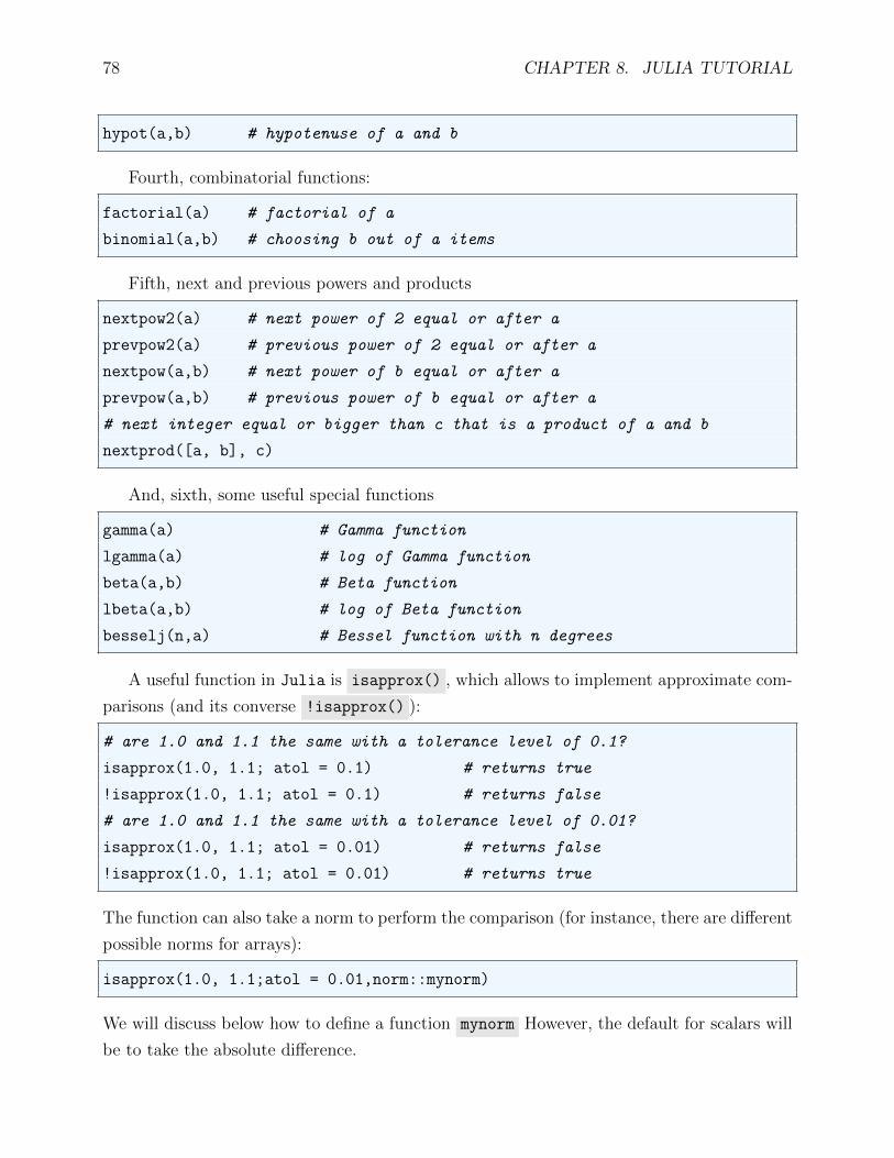
78 CHAPTER 8. JULIA TUTORIAL
hypot(a,b) # hypotenuse of a and b
Fourth, combinatorial functions:
factorial(a) # factorial of a
binomial(a,b) # choosing b out of a items
Fifth, next and previous powers and products
nextpow2(a) # next power of 2 equal or after a
prevpow2(a) # previous power of 2 equal or after a
nextpow(a,b) # next power of b equal or after a
prevpow(a,b) # previous power of b equal or after a
# next integer equal or bigger than c that is a product of a and b
nextprod([a, b], c)
And, sixth, some useful special functions
gamma(a) # Gamma function
lgamma(a) # log of Gamma function
beta(a,b) # Beta function
lbeta(a,b) # log of Beta function
besselj(n,a) # Bessel function with n degrees
A useful function in Julia is isapprox() , which allows to implement approximate com-
parisons (and its converse !isapprox() ):
# are 1.0 and 1.1 the same with a tolerance level of 0.1?
isapprox(1.0, 1.1; atol = 0.1) # returns true
!isapprox(1.0, 1.1; atol = 0.1) # returns false
# are 1.0 and 1.1 the same with a tolerance level of 0.01?
isapprox(1.0, 1.1; atol = 0.01) # returns false
!isapprox(1.0, 1.1; atol = 0.01) # returns true
The function can also take a norm to perform the comparison (for instance, there are different
possible norms for arrays):
isapprox(1.0, 1.1;atol = 0.01,norm::mynorm)
We will discuss below how to define a function mynorm However, the default for scalars will
be to take the absolute difference.
8.6. ARRAYS 79
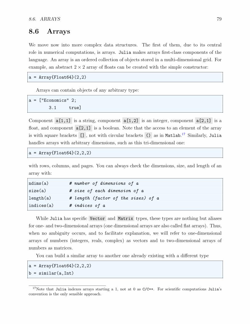
8.6 Arrays
We move now into more complex data structures. The first of them, due to its central
role in numerical computations, is arrays. Julia makes arrays first-class components of the
language. An array is an ordered collection of objects stored in a multi-dimensional grid. For
example, an abstract 2× 2 array of floats can be created with the simple constructor:
a = Array{Float64}(2,2)
Arrays can contain objects of any arbitrary type:
a = ["Economics" 2;
3.1 true]
Component a[1,1] is a string, component a[1,2] is an integer, component a[2,1] is a
float, and component a[2,1] is a boolean. Note that the access to an element of the array
is with square brackets [] , not with circular brackets () as in Matlab.17 Similarly, Julia
handles arrays with arbitrary dimensions, such as this tri-dimensional one:
a = Array{Float64}(2,2,2)
with rows, columns, and pages. You can always check the dimensions, size, and length of an
array with:
ndims(a) # number of dimensions of a
size(a) # size of each dimension of a
length(a) # length (factor of the sizes) of a
indices(a) # indices of a
While Julia has specific Vector and Matrix types, these types are nothing but aliases
for one- and two-dimensional arrays (one dimensional arrays are also called flat arrays). Thus,
when no ambiguity occurs, and to facilitate explanation, we will refer to one-dimensional
arrays of numbers (integers, reals, complex) as vectors and to two-dimensional arrays of
numbers as matrices.
You can build a similar array to another one already existing with a different type
a = Array{Float64}(2,2,2)
b = similar(a,Int)
17Note that Julia indexes arrays starting a 1, not at 0 as C/C++. For scientific computations Julia’sconvention is the only sensible approach.
80 CHAPTER 8. JULIA TUTORIAL
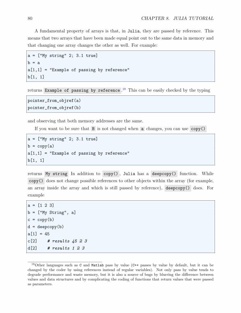
A fundamental property of arrays is that, in Julia, they are passed by reference. This
means that two arrays that have been made equal point out to the same data in memory and
that changing one array changes the other as well. For example:
a = ["My string" 2; 3.1 true]
b = a
a[1,1] = "Example of passing by reference"
b[1, 1]
returns Example of passing by reference .18 This can be easily checked by the typing
pointer_from_objref(a)
pointer_from_objref(b)
and observing that both memory addresses are the same.
If you want to be sure that B is not changed when a changes, you can use copy()
a = ["My string" 2; 3.1 true]
b = copy(a)
a[1,1] = "Example of passing by reference"
b[1, 1]
returns My string In addition to copy() , Julia has a deepcopy() function. While
copy() does not change possible references to other objects within the array (for example,
an array inside the array and which is still passed by reference), deepcopy() does. For
example
a = [1 2 3]
b = ["My String", a]
c = copy(b)
d = deepcopy(b)
a[1] = 45
c[2] # results 45 2 3
d[2] # results 1 2 3
18Other languages such as C and Matlab pass by value (C++ passes by value by default, but it can bechanged by the coder by using references instead of regular variables). Not only pass by value tends todegrade performance and waste memory, but it is also a source of bugs by blurring the difference betweenvalues and data structures and by complicating the coding of functions that return values that were passedas parameters.
8.6. ARRAYS 81
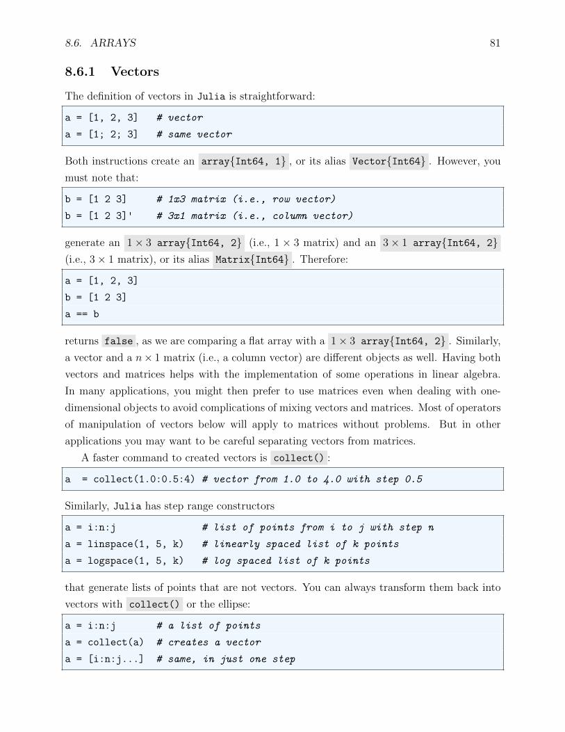
8.6.1 Vectors
The definition of vectors in Julia is straightforward:
a = [1, 2, 3] # vector
a = [1; 2; 3] # same vector
Both instructions create an array{Int64, 1} , or its alias Vector{Int64} . However, you
must note that:
b = [1 2 3] # 1x3 matrix (i.e., row vector)
b = [1 2 3]' # 3x1 matrix (i.e., column vector)
generate an 1× 3 array{Int64, 2} (i.e., 1 × 3 matrix) and an 3× 1 array{Int64, 2}(i.e., 3× 1 matrix), or its alias Matrix{Int64} . Therefore:
a = [1, 2, 3]
b = [1 2 3]
a == b
returns false , as we are comparing a flat array with a 1× 3 array{Int64, 2} . Similarly,
a vector and a n× 1 matrix (i.e., a column vector) are different objects as well. Having both
vectors and matrices helps with the implementation of some operations in linear algebra.
In many applications, you might then prefer to use matrices even when dealing with one-
dimensional objects to avoid complications of mixing vectors and matrices. Most of operators
of manipulation of vectors below will apply to matrices without problems. But in other
applications you may want to be careful separating vectors from matrices.
A faster command to created vectors is collect() :
a = collect(1.0:0.5:4) # vector from 1.0 to 4.0 with step 0.5
Similarly, Julia has step range constructors
a = i:n:j # list of points from i to j with step n
a = linspace(1, 5, k) # linearly spaced list of k points
a = logspace(1, 5, k) # log spaced list of k points
that generate lists of points that are not vectors. You can always transform them back into
vectors with collect() or the ellipse:
a = i:n:j # a list of points
a = collect(a) # creates a vector
a = [i:n:j...] # same, in just one step

82 CHAPTER 8. JULIA TUTORIAL
collect() is a generator that allows the use of general programming structures such as
loops or conditionals as the ones we will see in Section 8.7:
collect(x for x in 1:10 if isodd(x))
A related and versatile function is enumerate() , which returns an index of a collection
a=["micro","macro","econometrics"];
for (index, value) in enumerate(a)
println("$index$value")
end
# Prints
# 1 micro
# 2 macro
# 3 econometrics
The basic operators to manipulate vectors include:
show(a) # shows a
sum(a) # sum of a
maximum(a) # max of a
minimum(a) # min of a
dot(a, B) # inner product of two vectors
a[end] # gets last element of a
a[end-1] # gets element of a -1
Also, we can sort them:19
a = [2,1,3]
sort(a) # sorts a
sort(a,by=abs) # sorts a by absolute values
sortperm(a) # indices of sort of a
find the start and end
first(a) # returns 2
last(a) # returns 3
or any arbitrary elements in them:
19Sorting an array is a costly operation. Julia has four different sorting algorithms to do so depending onthe details of the array (you can change the defaults if you need to). Since this is more advanced material,you can check Julia’s documentation for details.

8.6. ARRAYS 83
a = [2,1,3]
first(a) # returns 2
last(a) # returns 3
find(isodd,a) # returns indices of occurrences (here 2,3)
findfirst(isodd,a) # returns first index of occurrence
# returns next index of occurrence
findnext(isodd,a,findfirst(a))
# returns next+b index of occurrence
findnext(isodd,a,findfirst(a)+b)
Note that we can check in any collection, including arrays, the presence of an element
with the short yet powerful function in :
a = [1,2,3]
2 in a # returns true
in(2,a) # same as above
4 in a # returns false
This is a good moment to introduce a Julia convention: the use of ! at the end of a
function. The suffix means that the function is changing the operand. For example:
sort!(a) # sorts a and changes it
shift!(a) # eliminates first element of a
unshift!(a,c) # adds c as an additional element of a at its start
pop!(a) # eliminates last element of a
push!(a,c) # adds c as an additional element of a at its end
To save space, we will not repeat the ! form of many of the functions that we will introduce
in the next paragraphs, but you can check the documentation about them in case you want
to use the version in your code.
Finally, Julia defines set operations
a = [2,1,3]
b = [2,4,5]
union(a,b) # returns 2,1,3,4,5
intersect(a,b) # returns 2
setdiff(a,b) # returns 1,3
setdiff(b,a) # returns 4,5
84 CHAPTER 8. JULIA TUTORIAL
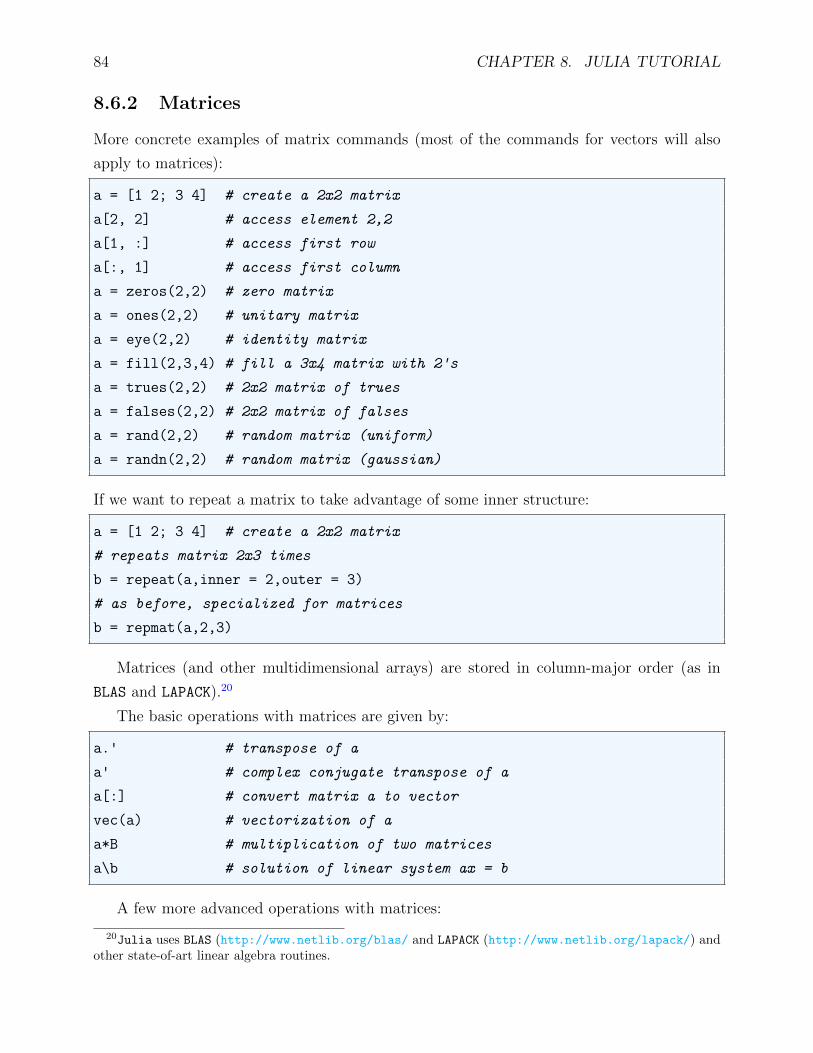
8.6.2 Matrices
More concrete examples of matrix commands (most of the commands for vectors will also
apply to matrices):
a = [1 2; 3 4] # create a 2x2 matrix
a[2, 2] # access element 2,2
a[1, :] # access first row
a[:, 1] # access first column
a = zeros(2,2) # zero matrix
a = ones(2,2) # unitary matrix
a = eye(2,2) # identity matrix
a = fill(2,3,4) # fill a 3x4 matrix with 2's
a = trues(2,2) # 2x2 matrix of trues
a = falses(2,2) # 2x2 matrix of falses
a = rand(2,2) # random matrix (uniform)
a = randn(2,2) # random matrix (gaussian)
If we want to repeat a matrix to take advantage of some inner structure:
a = [1 2; 3 4] # create a 2x2 matrix
# repeats matrix 2x3 times
b = repeat(a,inner = 2,outer = 3)
# as before, specialized for matrices
b = repmat(a,2,3)
Matrices (and other multidimensional arrays) are stored in column-major order (as in
BLAS and LAPACK).20
The basic operations with matrices are given by:
a.' # transpose of a
a' # complex conjugate transpose of a
a[:] # convert matrix a to vector
vec(a) # vectorization of a
a*B # multiplication of two matrices
a\b # solution of linear system ax = b
A few more advanced operations with matrices:
20Julia uses BLAS (http://www.netlib.org/blas/ and LAPACK (http://www.netlib.org/lapack/) andother state-of-art linear algebra routines.

8.6. ARRAYS 85
inv(a) # inverse of a
pinv(a) # pseudo-inverse of a
rank(a) # rank of a
norm(a) # Euclidean norm of a
det(a) # determinant of a
trace(a) # trace of a
val, vec = eig(a) # eigenvalues and eigenvectors
tril(a) # lower triangular matrix of a
triu(a) # upper triangular matrix of a
rot90(a,n) # rotate a 90 degrees n times
rot180(a,n) # rotate a 180 degrees n times
cat(i,a,b) # concatenate a and b along dimension i
a = [[1 2] [1 2]] # concatenate horizontally
vcat([1 2],[1 2]) # alternative notation to above
a = [[1 2]; [1 2]] # concatenate vertically
hcat([1 2],[1 2]) # alternative notation to above
a = diagm([1; 2; 3]) # diagonal matrix
a = reshape(1:10, 5, 2) # reshape
a = squeeze(a) # collapse a into 1 dimension
flipdim(a, 1) # flip up/down
flipdim(a, 2) # flip left/right
sortrows(a) # sorts rows lexicographically
sortcolumns(a) # sorts columns lexicographically
A powerful (but tricky!) function is broadcast() , which extends a non-conforming
matrix to the required dimensions in a function:
a = [1,2]
b = [1 2;3 4]
broadcast(+,a,b) # returns [2 3;5 6]
Finally, a few ascertain functions for matrices
issymmetric(a)
isposdef(a)
ishermitian(a)

86 CHAPTER 8. JULIA TUTORIAL
8.6.3 Sparse matrices
a = spzeros(100,100) # create a 100x100 sparse matrix
s = sparse(a) # converts dense matrix a into a sparse matrix s
a = full(s) # converts sparse matrix s into a dense matrix a
# finds indices for non-zero entries; returns two arrays for rows and
columns
findn(s)
# as before, plus a third array with the non-zero values
findnz(s)
8.6.4 Characters
Julia deals with characters with ease: they are regular objects that can be manipulated with
standard functions.
We can move between a Char and Int32 as follows:
Int32('a') # returns 97
Int64('a') # also returns 97
Int128('a') # also returns 97
Char(97) # returns a
and you can operate on them:
'a'+1 # returns b
You cannot, however, sum two characters (to avoid confusion with creating a string; see next
subsection).
8.6.5 Strings
Modern scientific computing is data intensive. Web scraping or data mining often required
intense search and manipulation of text. Thus, Julia has made string manipulation (i.e.,
dealing with finite sequences of characters) quite straightforward. More concretely, Julia
follows a syntax similar to the one of arrays and, therefore, you can extend most of what you
already know:
a ="I like economics" # string
b = a[1] # second component of string (here, 'I')
b = a[end] # last component of string (here, 's')

8.6. ARRAYS 87
Note that b is a character, not a string:
typeof(b) # returns Char
although we can make it a string with:
string(b) # returns "b"
and
b = a[1:1]
is a string. Also, \ and $ are not valid strings (like in LATEX). In particular, the operator $is used for variable interpolation in expressions (see below) and you can use $ as a substitute
if you need the currency sign.
Note that Julia uses " " for strings and ‘ ’ . If you want to have quotes inside the
string, you use triple quotes """
println("""I like economics "with" quotes""")
# returns I like economics "with" quotes
We can create strings by concatenating characters or smaller strings
string('a','b') # returns ab
string("a","b") # returns ab
"a"*"b" # returns ab
" " # white space
"a"*" "*"b" # returns a b
*("a","b") # returns ab
repeat("a",2) # returns aa
"a"^2 # returns aa also
join(["a","b"]," and ") # returns "a and b"
or randomly
randstring(n) # random string of n characters
We can insert a variable inside a string
a = 3
string("a=$a") # returns a=3
b = true
string(b) # returns "true"

88 CHAPTER 8. JULIA TUTORIAL
Note the use of operator $ to interpolate the variable a and the return of a boolean.
Some other commands to manipulate strings include
start("Economics") # returns 1
endof("Economics") # returns 9
next("Economics",2) # returns ('c',3)
uppercase("Economics") # returns ECONOMICS
lowercase("ECONOMICS") # returns economics
replace("Economics","cs","a") # returns Economia
reverse("Economics") # returns scimonocE
strip(" Economics ") # strips leading and trailing whitespace
lstrip(" Economics") # strips leading whitespace
rstrip("Economics ") # strips trailing whitespace
lpad("Economics",10) # returns Economics with left padding (10)
rpad("Economics",10) # returns Economics with right padding (10)
Searching in a string is done through search()
search("Economics","E") # returns 1:1 (from position 1 to 1)
search("Economics", "o") # returns 3:3 (first appearance of "o")
search("Economics", "Econ") # returns 1:4
search("Economics", "Macro") # returns 0:-1
ascertain of a substring through contains()
contains("Economics","E") # returns true
contains("Economics","M") # returns false
and splitting into substrings with split()
split("Economics","n") # returns ("Eco" "omics")
split("I like economics") # returns ("I" "like" "economics")
Julia also allows the standard syntax of regular expressions.21 When strings are compared
by logical operators, Julia follows a lexicographic order.
Finally, the ability of Julia to handle Unicode characters will allow you to use strings
with advanced mathematical symbols.
21See http://www.regular-expressions.info/reference.html for a complete reference.
8.6. ARRAYS 89
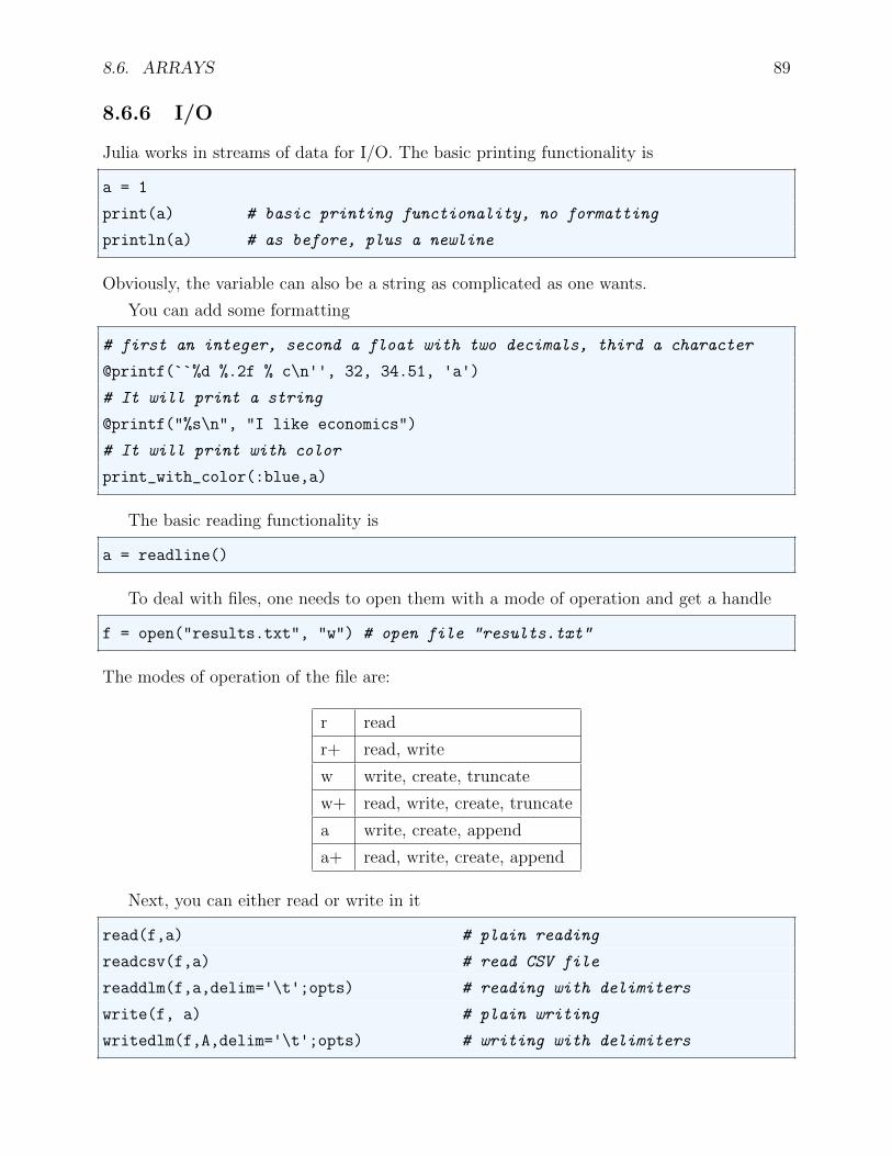
8.6.6 I/O
Julia works in streams of data for I/O. The basic printing functionality is
a = 1
print(a) # basic printing functionality, no formatting
println(a) # as before, plus a newline
Obviously, the variable can also be a string as complicated as one wants.
You can add some formatting
# first an integer, second a float with two decimals, third a character
@printf(``%d %.2f % c\n'', 32, 34.51, 'a')
# It will print a string
@printf("%s\n", "I like economics")
# It will print with color
print_with_color(:blue,a)
The basic reading functionality is
a = readline()
To deal with files, one needs to open them with a mode of operation and get a handle
f = open("results.txt", "w") # open file "results.txt"
The modes of operation of the file are:
r read
r+ read, write
w write, create, truncate
w+ read, write, create, truncate
a write, create, append
a+ read, write, create, append
Next, you can either read or write in it
read(f,a) # plain reading
readcsv(f,a) # read CSV file
readdlm(f,a,delim='\t';opts) # reading with delimiters
write(f, a) # plain writing
writedlm(f,A,delim='\t';opts) # writing with delimiters

90 CHAPTER 8. JULIA TUTORIAL
and close it
close(f)
An alternative, compact notation is
open("results.txt", "w") do f
write(f, "I like economics")
close(f)
end
open("results.txt", "r") do f
mystring = readdlm(f)
close(f)
end

8.7. PROGRAMMING STRUCTURES 91
8.7 Programming Structures
Julia has a flexible specification for functions (including abstract ones), MapReduce (a
particular set of functions), loops, and conditionals. We start our presentation discussing
functions in general.
8.7.1 Functions
In the tradition of programming languages in the functional approach, Julia considers func-
tions “first-class citizens” (i.e., an entity that can implement all the operations -which are
themselves functions- available to other entities). This means, among other things, that
Julia likes to work with functions without side effects and that you can follow the recent
boom in functional programming without jumping into purely functional language.
Recall that functions in Julia use methods with multiple dispatch: each function can
be associated with hundreds of different methods. Furthermore, you can add methods to an
already existing function.
There are two ways to create a function
# One-line
myfunction1(var) = var+1
# Several lines
function myfunction2(var1, var2="Float64", var3=1)
output1 = var1+2
output2 = var2+4
output3 = var3+3 # var3 is optional, by default var3=1
return output1 output2 output3
end
Note that tab indentation is not required by Julia; we only introduce it for visual appeal. In
the second function, var2 = ”Float64” fixed the type of the second argument and var3 = 1
pins a default value for the third argument, which becomes optional. We can also have
keyword argument, which can be ommitted
function myfunction3(var1, var2; keyword=2)
output1 = var1+var2+keyword
end
The difference between an optional argument and a keyword is that the keyword can appear
in any place of the function call while the optional argument must appear in order
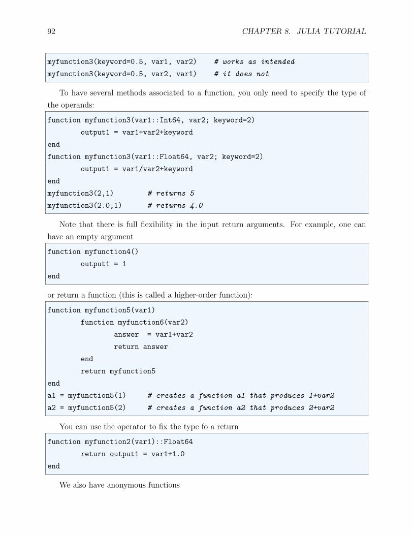
92 CHAPTER 8. JULIA TUTORIAL
myfunction3(keyword=0.5, var1, var2) # works as intended
myfunction3(keyword=0.5, var2, var1) # it does not
To have several methods associated to a function, you only need to specify the type of
the operands:
function myfunction3(var1::Int64, var2; keyword=2)
output1 = var1+var2+keyword
end
function myfunction3(var1::Float64, var2; keyword=2)
output1 = var1/var2+keyword
end
myfunction3(2,1) # returns 5
myfunction3(2.0,1) # returns 4.0
Note that there is full flexibility in the input return arguments. For example, one can
have an empty argument
function myfunction4()
output1 = 1
end
or return a function (this is called a higher-order function):
function myfunction5(var1)
function myfunction6(var2)
answer = var1+var2
return answer
end
return myfunction5
end
a1 = myfunction5(1) # creates a function a1 that produces 1+var2
a2 = myfunction5(2) # creates a function a2 that produces 2+var2
You can use the operator to fix the type fo a return
function myfunction2(var1)::Float64
return output1 = var1+1.0
end
We also have anonymous functions

8.7. PROGRAMMING STRUCTURES 93
x ->x^2 # anonymous function
a = x ->x^2 # named anonymous function
and you can define arrays of functions
a = [exp, abs]
8.7.2 Recursion, closures, and currying
abstract functions allow for easy coding of advanced techniques such as recursion, closures,
and currying. Recursions is a function that calls itself:
function outer(a)
b = a +2
function inner(b)
b = a+3
end
inner(b)
end
This is particularly useful for recursive computations, such as the canonical Fibonacci number
example:
fib(n) = n < 2 ? n : fib(n-1) + fib(n-2)
Unfortunately, recursions can be memory intensive and Julia does not implement tail call
(i.e., performed the required task at the very end of the recursion, and thus reducing memory
requirements to the same than would be required in a loop).
a closure is a record storing a function:
# We create a function that adds one
function counter()
n = 0
() -> n += 1
end
# we name it
addOne = counter()
addOne() # Produces 1
addOne() # Produces 2

94 CHAPTER 8. JULIA TUTORIAL
Closures allow for handling functions while keeping states hidden. This is known as continuation-
passing style (in contrast with the direct style of standard imperative programming).
Currying transforms the evaluation of a function with multiple arguments into the eval-
uation of a sequence of functions, each with a single argument:
function mult(a)
return function f(b)
return a*b
end
end
Currying allows for easier reuse of abstract functions and to avoid determining parameters
that are not required at the moment of evaluation.
Although in this tutorial we are not discussing the details of the LLVM-JIT compiler, you
can see the bitcode generated by some of these functions with:
code_llvm(x ->x^2, (Float64,))
You can also see the assembly code:
code_native(x ->x^2, (Float64,))
8.7.3 MapReduce
Julia supports generic function applicators. First, we have map() :
map(floor,[1.2, 5.6, 2.3]) # applies floor to vector [1.2, 5.6, 2.3]
map(x ->x^2,[1.2, 5.6, 2.3]) # applies abstract to vector [1.2, 5.6, 2.3]
map() also works for multiple inputs:
map((x,y) ->x+2*y,[1,2], [3,4])
An alternative syntax is with do-end
map([1.2, 5.6, 2.3]) do x
floor(x)
end
Second, we have reduce() and associated folding functions
reduce(+,[1,2,3]) # generic reduce
foldl(-,[1,2,3]) # folding (reduce) from the left
foldr(-,[1,2,3]) # folding (reduce) from the right
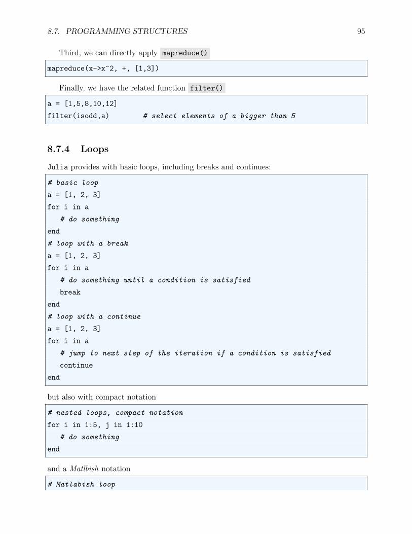
8.7. PROGRAMMING STRUCTURES 95
Third, we can directly apply mapreduce()
mapreduce(x->x^2, +, [1,3])
Finally, we have the related function filter()
a = [1,5,8,10,12]
filter(isodd,a) # select elements of a bigger than 5
8.7.4 Loops
Julia provides with basic loops, including breaks and continues:
# basic loop
a = [1, 2, 3]
for i in a
# do something
end
# loop with a break
a = [1, 2, 3]
for i in a
# do something until a condition is satisfied
break
end
# loop with a continue
a = [1, 2, 3]
for i in a
# jump to next step of the iteration if a condition is satisfied
continue
end
but also with compact notation
# nested loops, compact notation
for i in 1:5, j in 1:10
# do something
end
and a Matlbish notation
# Matlabish loop

96 CHAPTER 8. JULIA TUTORIAL
for i = 1:N
# do something
end
In contrast with other languages, in Julia if the counter variable did not exist before the
loop starts, it will be killed at the end of the loop.
Loops can be used to define arrays in comprehensions (a ruled-defined array)
[n^2 for n in 1:5] # basic comprehensions
Float64[n^2 for n in 1:5] # comprehension fixing type
Julia complements standard loops with comprehensions and whiles
# Comprehensions
[foo(i) for i in 1:5]
# basic while
while i <= N
# do something
end
8.7.5 Conditionals
Julia has both traditional if-then statements
if i <= N
# do something
elseif
# do something else
else
# do something even more different
end
and efficient ternary expressions condition ? do something : do something else such
as
a<2 ? b = 1 : b = 2
8.8. OTHER DATA STRUCTURES 97
8.8 Other Data Structures
Now it is a good time to introduce the more sophisticated data structures that Julia offers,
including user-defined ones.
8.8.1 Tuples
Tuples is a data type of that contains an ordered collection of elements. The elements of a
tuple cannot be changed once they have been defined
a = ("This is a tuple", 2018) # definition of a tuple
a[2] # accessing element 2 of tuple a
We can create tuples with zip
a = [1 2]
b = [3 4]
zip(a,b)
8.8.2 Dictionaries
Dictionaries are associative collections with keys (names of elements) are values of elements
# Creating a dictionary
a = Dict("University of Pennsylvania" => "Philadelphia", "Boston College" =>
"Boston")
a["University of Pennsylvania"] # access one key
a["Harvard"] = "Cambridge" # adds an additional key
delete!["Harvard"] # deletes a key
keys(a)
values(a)
haskey(a,"University of Pennsylvania") # returns true
haskey(a,"MIT") # returns false
Dictionaries are most convenient to deal with large sets of text.
8.8.3 Sets
[TBC]

98 CHAPTER 8. JULIA TUTORIAL
8.8.4 Composite types
Composite types are user-defined objects that store structured data. They are defined in
Julia with the construct struct . A good way to illustrate the usefulness of composite
types is to deal with a concrete example. Imagine that you have a survey of households
from the country of Deatonland. The survey, called MicroSurvey is done as in many other
countries, by recording detailed microdata from a representative sample of households for a
series of quarters. In each record, we have data with the id of the household (an integer),
the year of the survey (an integer), the quarter of the survey (an integer), the name of the
region in which the household resides (a string), the age of the household head in years
(an integer), the family size (an integer), the number children under 18 (an integer), and
the total consumption expenditure in the quarter (a floating). The Survey of Consumer
Expenditures in the U.S. and similar surveys in other countries have a structure close to
this one, only with even richer information.22
You want to read, store, and manipulate the information from the survey, perhaps with
thousands of observations. You soon realize that you have plenty of data that comes in a
non-conventional form: part of it is in terms of integers, part in terms of a string, part in
terms of a floating, etc. In some datasets, the information may even contain complex Unicode
characters, images, maps, etc. You could construe arrays to store that information (Julia
allows for arrays with multiple types), but, after some time you will find that the approach
generates complex code.
a much simpler strategy is to design your own type. In particular, we can define a type
called MicroSurveyObservation . To do so, we invoke a construct struct followed by a
block of field names and closed by end . More concretely, the syntax is
struct MicroSurveyObservation
id::Int
year::Int
quarter::Int
region::String
ageHouseholdHead::Int
familySize::Int
numberChildrenunder18::Int
consumption::Float64
end
22In fact, we deal with an abstract survey to emphasize how general the technique of composite types is.We could be dealing with a survey of firms, a panel of establishments, social security records, census tractinformation, or any of the other myriad of forms in which micro data comes.

8.8. OTHER DATA STRUCTURES 99
In this example, we have annotated all fields with the operator :: . This is not necessary: a
field not annotated will default to any , as in this alternative formulation:
# alternative constructor of MicroSurveyObservation
struct MicroSurveyObservation
id
# other fields here
end
Creating an instance of MicroSurveyObservation is straightforward:
household1 = MicroSurveyObservation(12,2017,3,"angushire",23,2,0,345.34)
household1 is an instance with id=12, observed in the year 2017.Q3, which lives in the
region of “angushire,” where the head of the household is 23 years old, where there are
2 people in the household, none of them a child under 18, and with a total consumption
expenditure of 354.34 units.
If we try to create a instance with the wrong type in one of the fields:
household1 = MicroSurveyObservation(12,2017,3,"angushire",23,2.3,0,345.34)
we will get an error message InexactError() : a household cannot have a size of 2.3!
You can check the names of all the fields with
fieldnames(MicroSurveyObservation)
To access to any of these fields, you only need to use a . after the name of the variable
followed by the field:
household1.family_size
returns 2 . Also, we can use household1.familySize to operate as you would do with
other values:
totalPopulation = household1.familySize
However, household1 , like any other object created by struct , is immutable. If you
try to change id from 12 to 31:
household1.id = 31
you would get type MicroSurveyObservation is immutable . In the next subsection, we
will introduce mutable composite types and discuss why it makes sense that the default is
immutability.
100 CHAPTER 8. JULIA TUTORIAL
Obviously creating a different variable for each observation in our survey is not very
efficient. Imagine that we have 10 observations. Then, we can define an abstract array 10×1
and populate it with repeated applications of the constructor:
household = array{any}(10,1)
household[1] = MicroSurveyObservation(12,2017,3,"angushire", 23, 2,0,345.34)
household[2] = MicroSurveyObservation(13,2015,2,"Wolpex", 35, 5,2,645.34)
...
Even more efficiently, you can build a loop that reads data from a file and builds each element
of the array:
household = array{any}(10,1)
for i in 1:10
# read file with observation
household[1] = MicroSurveyObservation(#data from previous step)
end
If you have experience with other object-oriented languages you would have recognized
that a composite type is similar to a class in C++, Python, R, or Matlab or a structure in
C/C++ or Matlab.23 at the same time, you might miss the definition of methods in the class.
In comparison with object-oriented languages, in Julia functions are not tied with objects.
This is a second key difference of multiple dispatch with respect to operator overloading: in
Julia you will take an existing function and add a new method to it to deal with a concrete
composite type or create a new function with its specific method if you want to have a
completely new operation.
an example of adding a new method is
# importing + from base package
import Base: +
# definition of sum function for MicroSurveyObservation composite types
(x::MicroSurveyObservation,y::MicroSurveyObservation) = x.consumption + y.
consumption
# an example of how to apply the sum
household[1]+household[2]
23Originally Matlab only had structures, classes were added later on; to maintain the language backward-compatible, both types survive. Something similar happens in C++ to maintain nearly all C programs com-patible.

8.8. OTHER DATA STRUCTURES 101
This function extends the sum operator + to instances of MicroSurveyObservation . We
first import Base: + and then specify that a sum in this context means summing the
total consumption expenditure of both households. This function returns 991... . Obviously
there is nothing special about defining the sum operator on total consumption expenditure.
We could have done it, for example, on total household size.
an example of a new function is:
equivConsumption(x::MicroSurveyObservation) = x.consumption/sqrt(x.
familySize)
Why do we want to divide these two fields? Many economists have highlighted the presence
of increasing returns to scale in household consumption: when the size of a household goes
from 1 to 2, total household consumption expenditure does not need to double to produce the
same level of utility than before the increase. For example, a household of 2 only needs one
Netflix subscription, exactly the same than a household of 1. A rough approximation to the
economies of scale estimated by researchers is that consumption needs grow with the square
root of household size: a household of 2 requires√
(2) units of consumption.24 To implement
this idea, equivConsumption() takes an instance of of MicroSurveyObservation , extracts
its information on consumption and family size and computes the equivalence scale.
Note the flexibility of working with composite types in this way: if you decide to define a
new household equivalence scale you only need to change the function equivConsumption()
without worrying about the data structure itself. In comparison, with classes in C++ or
Matlab, you would need to change the definition of the class itself by introducing a new
operator.
8.8.5 Mutable Composite Types
Sometimes it is convenient to have composite types that are mutable.
mutable struct MicroSurveyObservation
id::Int
...
end
The default, however, is of immutability. An immutable object can safely be stored in
memory and passed by copy. This makes the code more efficient and safer. In particular, a
24There is a large literature on household equivalence scale that we do not need to review here. Moresophisticated scales take care of issues such distinguishing between adults and children, age of the children,etc.

102 CHAPTER 8. JULIA TUTORIAL
function cannot accidentally change a field value. When you are dealing with complex types
such as composite ones, functions may have unexpected effects. A mutable object will be
stored in the heap and have a stable memory address.
8.8.6 Parametric Composite Types
[TBC]
8.8.7 Type Union
[TBC]
8.9 Metaprogramming
Metaprogramming writes code that can modify itself. One natural application is for writing
repetitive code: if you can come up, for example, for a rule of how to define a large number
of arrays, perhaps you can write a code that writes the code to define all these arrays. Julia,
influenced by Lisp, has a strong metaprogramming orientation.25
A simple instance of metaprogramming, which you might have seen in other contexts, is
macros, blocks of code that can be recycled:
macro welcome(name)
return :(println("Hello ", $name, " likes economics"))
end
@welcome("Jesus")
But Julia offers more sophisticated capabilities. First, note that every task in Julia is
an expression. You can get a handle of that expression with quote()-end
a = quote
"I like economics"
end
typeof(a) # returns Expr
If you then apply eval()
eval(a)
25In fact, some knowledge of Lisp or a more modern descendant such as Clojure is a great complementfor those economists who acquire an advanced level of proficiency with Julia.
8.10. PLOTS 103
the console will print I like economics .
A more concise notation to define an expression is with the operator :
:(a = "I like economics")
Thus, you can build code such as
name = "Jesus"
a = :(name*" likes economics")
eval(a) # returns "Jesus likes economics"
name = "Pablo"
eval(a) # returns "Pablo likes economics"
This, for example, will allow you to build files of data changing a variable. If you modify the
expression to
a = :($name*" likes economics")
you can also see the vale of “name” in any given moment.
We can look at the fields of the expression with fieldnames() and the whole details
with dump()
fieldnames(a)
dump(a)
Each of the fields can be accessed with .
a.args
# returns
# Any[2]
# console, line 1:
# "I like economics"
which allows you to change them
a.args[2] = "I really like economics"
eval(a) # prints "I really like economics"
8.10 Plots
Julia’s base package does not include plotting capabilities. This allows the use of differ-
ent packages to adapt to the needs of each user and to separate plotting from numerical
considerations.
104 CHAPTER 8. JULIA TUTORIAL
A simple plot can be done with the Plots package
using Plots
x = 1:10
y = x.^2
plot(x,y)
From now on, we will assume that Plots has already been imported
A more sophisticated plot, still using Plots
square(x) = x^2
plot(square,1:10,title="A nice plot", label = "Square function",line = (:
blue,0.9,3, :dot), xlabel = "x-axis", ylabel ="y-axis")
cube(x) = x^3
plot!(cube,1:10, label = "Cube function",line =(:red,0.9,3, :dot))
savefig("figure1.pdf")
where we have added a second line (note the suffix).
A scatter plot
x = 1:10
y = x.^2
Plots.scatter(x,y,label = "3d plot",line =(:red,0.9,3, :dot))
Several other plots:
x = 1:10
Plots.pie(x) # a pie-chart
Plots.bar(x) # a bar-chart
Plots.histogram(x) # a histogram
A 3-d graph:
x = 1:10
y = x.^2
z = x.^3
Plots.plot3d(x,y,z,label = "3d plot",line =(:red,0.9,3, :dot))
8.11 Random Numbers
randn(10) # a draw from a standardized normal distribution

8.12. MULTIPLE FILES 105
8.12 Multiple Files
include("myfunctions.jl")
Files need to be in the present working directory, which you can determine with pwd()
8.13 Timing
time() # current time
tic() # start time counter
toc() # end time counter
@time main() # Measures time execution of main()
Note that @time is a built-in macro.
8.14 Parallel
Julia has been designed for straightforward parallelization. The first step is to add workers
to a task
addprocs(2)
Next, we can have a parallel loop
simulation = Sharedarray{Float64}(100)
@parallel for i in 1:100
simulation[i] = i
end
8.15 Some Advanced Topics
We conclude with some advanced functionality. We will assume now that you have more ex-
perience with programming to appreciate the essence of each topic without much explanation.
First, try-catch errors follow a syntax of the form:
function square(x)
try
sqrt(x)

106 CHAPTER 8. JULIA TUTORIAL
catch err
println(err)
end
end
square(2) # returns 1.41...
square("economics") # returns MethodError(sqrt, ("economics",), 0....)
8.16 A Worked-out Example
## Basic RBC model with full depreciation
#
# Jesus Fernandez-Villaverde
# Haverford, July 29, 2013
function main()
## 1. Calibration
aalpha = 1/3 # Elasticity of output w.r.t. capital
bbeta = 0.95 # Discount factor
# Productivity values
vProductivity = [0.9792 0.9896 1.0000 1.0106 1.0212]
# Transition matrix
mTransition = [0.9727 0.0273 0.0000 0.0000 0.0000;
0.0041 0.9806 0.0153 0.0000 0.0000;
0.0000 0.0082 0.9837 0.0082 0.0000;
0.0000 0.0000 0.0153 0.9806 0.0041;
0.0000 0.0000 0.0000 0.0273 0.9727]
# 2. Steady State
capitalSteadyState = (aalpha*bbeta)^(1/(1-aalpha))
outputSteadyState = capitalSteadyState^aalpha
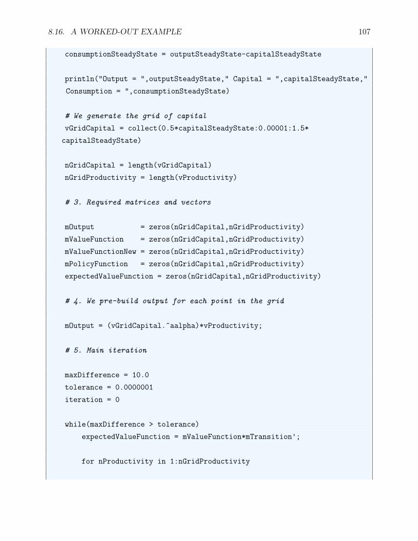
8.16. A WORKED-OUT EXAMPLE 107
consumptionSteadyState = outputSteadyState-capitalSteadyState
println("Output = ",outputSteadyState," Capital = ",capitalSteadyState,"
Consumption = ",consumptionSteadyState)
# We generate the grid of capital
vGridCapital = collect(0.5*capitalSteadyState:0.00001:1.5*
capitalSteadyState)
nGridCapital = length(vGridCapital)
nGridProductivity = length(vProductivity)
# 3. Required matrices and vectors
mOutput = zeros(nGridCapital,nGridProductivity)
mValueFunction = zeros(nGridCapital,nGridProductivity)
mValueFunctionNew = zeros(nGridCapital,nGridProductivity)
mPolicyFunction = zeros(nGridCapital,nGridProductivity)
expectedValueFunction = zeros(nGridCapital,nGridProductivity)
# 4. We pre-build output for each point in the grid
mOutput = (vGridCapital.^aalpha)*vProductivity;
# 5. Main iteration
maxDifference = 10.0
tolerance = 0.0000001
iteration = 0
while(maxDifference > tolerance)
expectedValueFunction = mValueFunction*mTransition';
for nProductivity in 1:nGridProductivity

108 CHAPTER 8. JULIA TUTORIAL
# We start from previous choice (monotonicity of policy
function)
gridCapitalNextPeriod = 1
for nCapital in 1:nGridCapital
valueHighSoFar = -1000.0
capitalChoice = vGridCapital[1]
for nCapitalNextPeriod in gridCapitalNextPeriod:nGridCapital
consumption = mOutput[nCapital,nProductivity]-
vGridCapital[nCapitalNextPeriod]
valueProvisional = (1-bbeta)*log(consumption)+bbeta*
expectedValueFunction[nCapitalNextPeriod,nProductivity]
if (valueProvisional>valueHighSoFar)
valueHighSoFar = valueProvisional
capitalChoice = vGridCapital[
nCapitalNextPeriod]
gridCapitalNextPeriod = nCapitalNextPeriod
else
break # We break when we have achieved the
max
end
end
mValueFunctionNew[nCapital,nProductivity] = valueHighSoFar
mPolicyFunction[nCapital,nProductivity] = capitalChoice
end
end
maxDifference = maximum(abs.(mValueFunctionNew-mValueFunction))
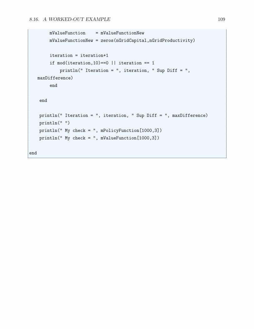
8.16. A WORKED-OUT EXAMPLE 109
mValueFunction = mValueFunctionNew
mValueFunctionNew = zeros(nGridCapital,nGridProductivity)
iteration = iteration+1
if mod(iteration,10)==0 || iteration == 1
println(" Iteration = ", iteration, " Sup Diff = ",
maxDifference)
end
end
println(" Iteration = ", iteration, " Sup Diff = ", maxDifference)
println(" ")
println(" My check = ", mPolicyFunction[1000,3])
println(" My check = ", mValueFunction[1000,3])
end

110 CHAPTER 8. JULIA TUTORIAL
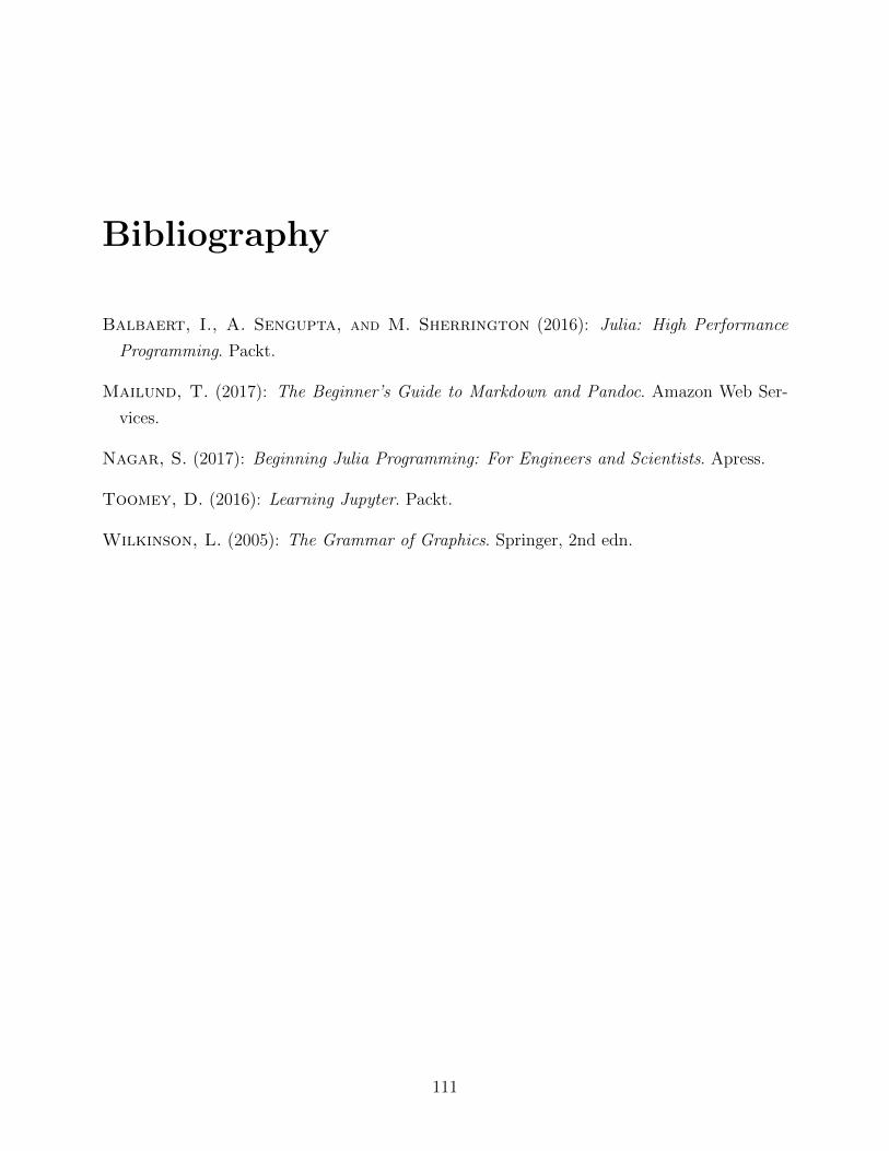
Bibliography
Balbaert, I., A. Sengupta, and M. Sherrington (2016): Julia: High Performance
Programming. Packt.
Mailund, T. (2017): The Beginner’s Guide to Markdown and Pandoc. Amazon Web Ser-
vices.
Nagar, S. (2017): Beginning Julia Programming: For Engineers and Scientists. Apress.
Toomey, D. (2016): Learning Jupyter. Packt.
Wilkinson, L. (2005): The Grammar of Graphics. Springer, 2nd edn.
111