© 2002 Thomson / South-Western Slide 9-1 Chapter 9 Hypothesis Testing with Single Samples.

1
Hypothesis Testing with
Two Samples
Chapter 8
§ 8.1
Testing the Difference
Between Means (Large
Independent Samples)
Larson & Farber, Elementary Statistics: Picturing the World, 3e 3
Two Sample Hypothesis Testing
In a two-sample hypothesis test, two parameters from two
populations are compared.
For a two-sample hypothesis test,
1. the null hypothesis H0 is a statistical hypothesis that usually
states there is no difference between the parameters of two
populations. The null hypothesis always contains the symbol ≤, =, or ≥.
2. the alternative hypothesis Ha is a statistical hypothesis that is
true when H0 is false. The alternative hypothesis always
contains the symbol >, ≠, or <.

2
Larson & Farber, Elementary Statistics: Picturing the World, 3e 4
Two Sample Hypothesis Testing
To write a null and alternative hypothesis for a two-sample
hypothesis test, translate the claim made about the population
parameters from a verbal statement to a mathematical statement.
H0: µ1 = µ2
Ha: µ1 ≠ µ2
H0: µ1 ≤ µ2Ha: µ1 > µ2
H0: µ1 ≥ µ2Ha: µ1 < µ2
Regardless of which hypotheses used, µ1 = µ2 is always
assumed to be true.
Larson & Farber, Elementary Statistics: Picturing the World, 3e 5
Two Sample z-Test
Three conditions are necessary to perform a z-test for the
difference between two population means µ1 and µ2.
1. The samples must be randomly selected.
2. The samples must be independent. Two samples are
independent if the sample selected from one population is
not related to the sample selected from the second
population.
3. Each sample size must be at least 30, or, if not, each
population must have a normal distribution with a known
standard deviation.
Larson & Farber, Elementary Statistics: Picturing the World, 3e 6
Two Sample z-Test
If these requirements are met, the sampling distribution for
(the difference of the sample means) is a normal distribution with
mean and standard error of
1 2 1 21 2x x x xµ µ µ µ µ− = − = −
1 2x x−
and
1 2 1 2
2 22 2 1 2
1 2
.x x x x
σ σσ σ σ
n n− = + = +
1 2µ µ−1 2x xσ −−
1 2x xσ −
Sampling distribution
for 1 2x x− 1 2x x−
3
Larson & Farber, Elementary Statistics: Picturing the World, 3e 7
Two Sample z-Test
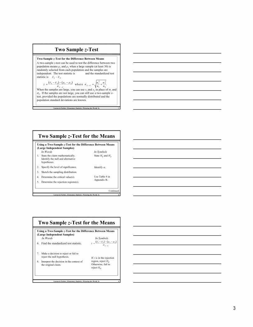
Two-Sample z-Test for the Difference Between Means
A two-sample z-test can be used to test the difference between two
population means µ1 and µ2 when a large sample (at least 30) is
randomly selected from each population and the samples are
independent. The test statistic is and the standardized test
statistic is
When the samples are large, you can use s1 and s2 in place of σ1 and σ2. If the samples are not large, you can still use a two-sample z-test, provided the populations are normally distributed and the
population standard deviations are known.
( ) ( )1 2
1 2
2 21 2 1 2 1 2
1 2
where .x xx x
x x µ µ σ σz σ
σ n n−−
− − −= = +
1 2x x−
Larson & Farber, Elementary Statistics: Picturing the World, 3e 8
Two Sample z-Test for the Means
1. State the claim mathematically.
Identify the null and alternative
hypotheses.
2. Specify the level of significance.
3. Sketch the sampling distribution.
4. Determine the critical value(s).
5. Determine the rejection regions(s).
Continued.
Using a Two-Sample z-Test for the Difference Between Means
(Large Independent Samples)
In Words In Symbols
State H0 and Ha.
Identify α.
Use Table 4 in
Appendix B.
Larson & Farber, Elementary Statistics: Picturing the World, 3e 9
Two Sample z-Test for the Means
In Words In Symbols
If z is in the rejection
region, reject H0.
Otherwise, fail to
reject H0.
6. Find the standardized test statistic.
7. Make a decision to reject or fail to
reject the null hypothesis.
8. Interpret the decision in the context of
the original claim.
Using a Two-Sample z-Test for the Difference Between Means
(Large Independent Samples)
( ) ( )1 2
1 2 1 2
x x
x x µ µz
σ −
− − −=
4
Larson & Farber, Elementary Statistics: Picturing the World, 3e 10
Two Sample z-Test for the Means
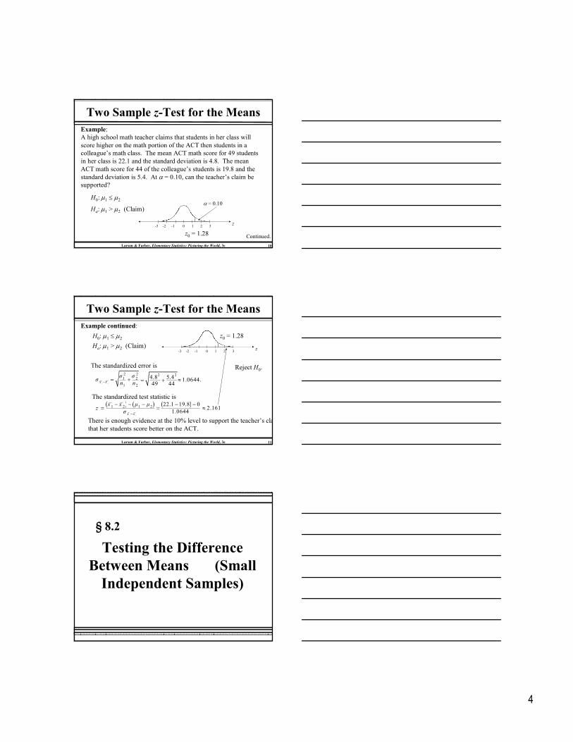
Example:
A high school math teacher claims that students in her class will
score higher on the math portion of the ACT then students in a
colleague’s math class. The mean ACT math score for 49 students
in her class is 22.1 and the standard deviation is 4.8. The mean
ACT math score for 44 of the colleague’s students is 19.8 and the
standard deviation is 5.4. At α = 0.10, can the teacher’s claim be
supported?
Ha: µ1 > µ2 (Claim)
H0: µ1 ≤ µ2
Continued.z0 = 1.28
z0 1 2 3-3 -2 -1
α = 0.10
Larson & Farber, Elementary Statistics: Picturing the World, 3e 11
Two Sample z-Test for the Means
( ) ( )1 2
1 2 1 2
x x
x x µ µz
σ −
− − −=
Example continued:
The standardized error is
( )22.1 19.8 0
1.0644
− −=
Ha: µ1 > µ2 (Claim)
H0: µ1 ≤ µ2
1 2
2 21 2
1 2x x
σ σσ
n n− = + 1.0644.≈2 24.8 5.4
49 44= +
The standardized test statistic is
2.161≈
z0 = 1.28
z0 1 2 3-3 -2 -1
Reject H0.
There is enough evidence at the 10% level to support the teacher’s claim
that her students score better on the ACT.
§ 8.2
Testing the Difference
Between Means (Small
Independent Samples)
5
Larson & Farber, Elementary Statistics: Picturing the World, 3e 13
Two Sample t-Test
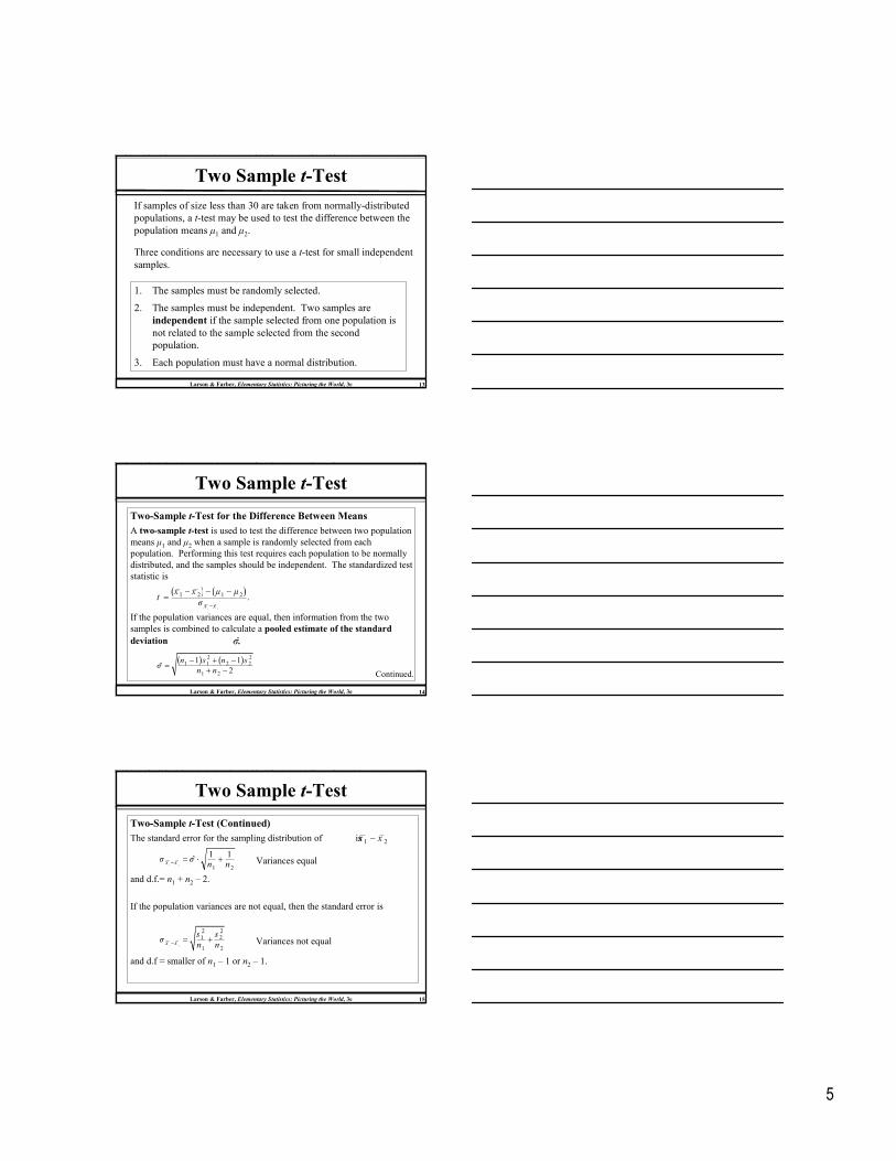
1. The samples must be randomly selected.
2. The samples must be independent. Two samples are
independent if the sample selected from one population is
not related to the sample selected from the second
population.
3. Each population must have a normal distribution.
If samples of size less than 30 are taken from normally-distributed
populations, a t-test may be used to test the difference between the
population means µ1 and µ2.
Three conditions are necessary to use a t-test for small independent
samples.
Larson & Farber, Elementary Statistics: Picturing the World, 3e 14
Two Sample t-Test
Two-Sample t-Test for the Difference Between Means
A two-sample t-test is used to test the difference between two population
means µ1 and µ2 when a sample is randomly selected from each
population. Performing this test requires each population to be normally
distributed, and the samples should be independent. The standardized test
statistic is
If the population variances are equal, then information from the two
samples is combined to calculate a pooled estimate of the standard
deviation
( ) ( )1 2
1 2 1 2 . x x
x x µ µt
σ −
− − −=
σ̂.
( ) ( )2 21 1 2 2
1 2
1 1ˆ
2
n s n sσ
n n
− + −=
+ − Continued.
Larson & Farber, Elementary Statistics: Picturing the World, 3e 15
Two Sample t-Test
Two-Sample t-Test (Continued)
The standard error for the sampling distribution of is
and d.f.= n1 + n2 – 2.
If the population variances are not equal, then the standard error is
and d.f = smaller of n1 – 1 or n2 – 1.
1 2
1 2
1 1ˆx xσ σ
n n− = ⋅ +
1 2x x−
Variances equal
1 2
2 21 2
1 2x x
s sσ
n n− = + Variances not equal
6
Larson & Farber, Elementary Statistics: Picturing the World, 3e 16
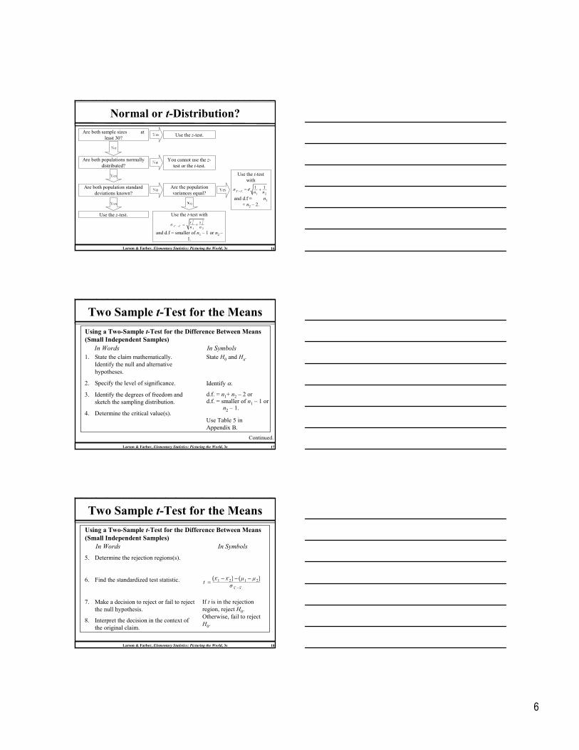
Normal or t-Distribution?
Are both sample sizes at
least 30?
Are both populations normally
distributed?
You cannot use the z-
test or the t-test.
No
Yes
Are both population standard
deviations known?
Use the z-test.Yes
No
Are the population
variances equal?
Use the z-test. Use the t-test with
and d.f = smaller of n1 – 1 or n2 –
1.
1 2
2 21 2
1 2
x x
s sσ
n n− = +
Use the t-test
with
and d.f = n1+ n2 – 2.
1 2
1 2
1 1 ˆx xσ σ
n n− = +
Yes
No
No
Yes
Larson & Farber, Elementary Statistics: Picturing the World, 3e 17
Two Sample t-Test for the Means
1. State the claim mathematically.
Identify the null and alternative
hypotheses.
2. Specify the level of significance.
3. Identify the degrees of freedom and
sketch the sampling distribution.
4. Determine the critical value(s).
Continued.
Using a Two-Sample t-Test for the Difference Between Means
(Small Independent Samples)
In Words In Symbols
State H0 and Ha.
Identify α.
Use Table 5 in
Appendix B.
d.f. = n1+ n2 – 2 ord.f. = smaller of n1 – 1 or
n2 – 1.
Larson & Farber, Elementary Statistics: Picturing the World, 3e 18
Two Sample t-Test for the Means
In Words In Symbols
If t is in the rejection
region, reject H0.
Otherwise, fail to reject
H0.
5. Determine the rejection regions(s).
6. Find the standardized test statistic.
7. Make a decision to reject or fail to reject
the null hypothesis.
8. Interpret the decision in the context of
the original claim.
Using a Two-Sample t-Test for the Difference Between Means
(Small Independent Samples)
( ) ( )1 2
1 2 1 2
x x
x x µ µt
σ −
− − −=
7
Larson & Farber, Elementary Statistics: Picturing the World, 3e 19
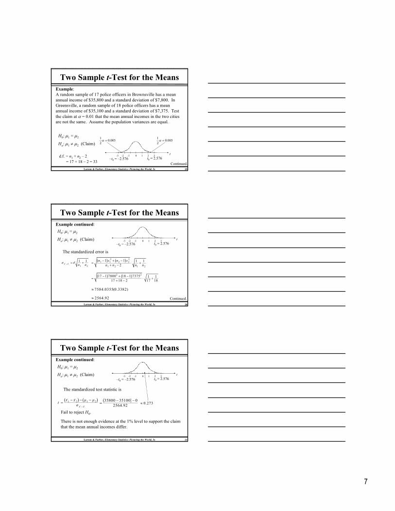
Two Sample t-Test for the Means
Example:
A random sample of 17 police officers in Brownsville has a mean
annual income of $35,800 and a standard deviation of $7,800. In
Greensville, a random sample of 18 police officers has a mean
annual income of $35,100 and a standard deviation of $7,375. Test
the claim at α = 0.01 that the mean annual incomes in the two cities
are not the same. Assume the population variances are equal.
Ha: µ1 ≠ µ2 (Claim)
H0: µ1 = µ2
Continued.
–t0 = –2.576d.f. = n1 + n2 – 2
= 17 + 18 – 2 = 33t0 = 2.576
t0 1 2 3-3 -2 -1
005.02
1=α 005.0
2
1=α
Larson & Farber, Elementary Statistics: Picturing the World, 3e 20
Two Sample t-Test for the Means
Example continued:
The standardized error is
1 2
1 2
1 1 ˆx xσ σ
n n− = +
( ) ( )2 217 1 7800 18 1 7375 1 117 18 2 17 18
− + −= ⋅ +
+ −
( ) ( )2 21 1 2 2
1 2 1 2
1 1 1 12
n s n s
n n n n
− + −= ⋅ +
+ −
Ha: µ1 ≠ µ2 (Claim)
H0: µ1 = µ2
–t0 = –2.576
t0 1 2 3-3 -2 -1
t0 = 2.576
7584.0355(0.3382)≈
Continued.2564.92≈
Larson & Farber, Elementary Statistics: Picturing the World, 3e 21
Two Sample t-Test for the Means
( ) ( )1 2
1 2 1 2
x x
x x µ µt
σ −
− − −=
Example continued:
The standardized test statistic is
0.273≈
Fail to reject H0.
There is not enough evidence at the 1% level to support the claim
that the mean annual incomes differ.
Ha: µ1 ≠ µ2 (Claim)
H0: µ1 = µ2
–t0 = –2.576
t0 1 2 3-3 -2 -1
t0 = 2.576
( )35800 35100 0
2564.92
− −=

8
§ 8.3
Testing the Difference
Between Means
(Dependent Samples)
Larson & Farber, Elementary Statistics: Picturing the World, 3e 23
Two samples are independent if the sample selected from one
population is not related to the sample selected from the second
population. Two samples are dependent if each member of one
sample corresponds to a member of the other sample. Dependent
samples are also called paired samples or matched samples.
Independent and Dependent Samples
Independent Samples Dependent Samples
Larson & Farber, Elementary Statistics: Picturing the World, 3e 24
Example:
Classify each pair of samples as independent or dependent.
Independent and Dependent Samples
Sample 1: The weight of 24 students in a first-grade class
Sample 2: The height of the same 24 students
These samples are dependent because the weight and height can
be paired with respect to each student.
Sample 1: The average price of 15 new trucks
Sample 2: The average price of 20 used sedans
These samples are independent because it is not possible to pair
the new trucks with the used sedans. The data represents prices
for different vehicles.

9
Larson & Farber, Elementary Statistics: Picturing the World, 3e 25
t-Test for the Difference Between Means
To perform a two-sample hypothesis test with dependent samples,
the difference between each data pair is first found:
Three conditions are required to conduct the test.
d = x1 – x2 Difference between entries for a data pair.
The test statistic is the mean of these differences.d
.d
dn∑=
Mean of the differences between paired data
entries in the dependent samples.
Larson & Farber, Elementary Statistics: Picturing the World, 3e 26
t-Test for the Difference Between Means
1. The samples must be randomly selected.
2. The samples must be dependent (paired).
3. Both populations must be normally distributed.
d
If these conditions are met, then the sampling distribution for is
approximated by a t-distribution with n – 1 degrees of freedom,
where n is the number of data pairs.
d–t0 t0µd
Larson & Farber, Elementary Statistics: Picturing the World, 3e 27
t-Test for the Difference Between Means
The following symbols are used for the t-test for .dµ
DescriptionSymbol
n The number of pairs of data
d The difference between entries for a data pair, d = x1 – x2
dµ The hypothesized mean of the differences of paired data in the
population
d The mean of the differences between the paired data entries in the
dependent samples
dsThe standard deviation of the differences between the paired data
entries in the dependent samples
dd
n∑=
( )22( )
( 1)d
n d ds
n n
∑ − ∑=
−

10
Larson & Farber, Elementary Statistics: Picturing the World, 3e 28
t-Test for the Difference Between Means
t-Test for the Difference Between Means
A t-test can be used to test the difference of two population means when a
sample is randomly selected from each population. The requirements for
performing the test are that each population must be normal and each
member of the first sample must be paired with a member of the second
sample.
The test statistic is
and the standardized test statistic is
The degrees of freedom are
d.f. = n – 1.
.d
d
d µt
s n
−=
dd
n∑=
Larson & Farber, Elementary Statistics: Picturing the World, 3e 29
t-Test for the Difference Between Means
1. State the claim mathematically.
Identify the null and alternative
hypotheses.
2. Specify the level of significance.
3. Identify the degrees of freedom and
sketch the sampling distribution.
4. Determine the critical value(s).
Continued.
Using the t-Test for the Difference Between Means
(Dependent Samples)
In Words In Symbols
State H0 and Ha.
Identify α.
Use Table 5 in
Appendix B.
d.f. = n – 1
Larson & Farber, Elementary Statistics: Picturing the World, 3e 30
t-Test for the Difference Between Means
In Words In Symbols
5. Determine the rejection region(s).
6. Calculate and Use a table.
7. Find the standardized test statistic.
Using a Two-Sample t-Test for the Difference Between Means
(Small Independent Samples)
dd
n∑=d .ds
2 2( ) ( )
( 1)d
n d ds
n n
∑ − ∑=−
d
d
d µt
s n
−=
11
Larson & Farber, Elementary Statistics: Picturing the World, 3e 31
t-Test for the Difference Between Means
In Words In Symbols
If t is in the rejection
region, reject H0.
Otherwise, fail to
reject H0.
8. Make a decision to reject or fail to
reject the null hypothesis.
9. Interpret the decision in the context
of the original claim.
Using a Two-Sample t-Test for the Difference Between Means
(Small Independent Samples)
Larson & Farber, Elementary Statistics: Picturing the World, 3e 32
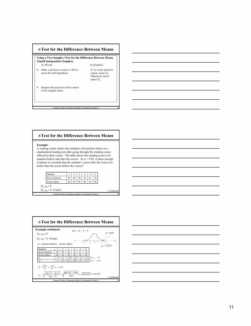
t-Test for the Difference Between Means
Example:
A reading center claims that students will perform better on a
standardized reading test after going through the reading course
offered by their center. The table shows the reading scores of 6
students before and after the course. At α = 0.05, is there enough
evidence to conclude that the students’ scores after the course are
better than the scores before the course?
Continued.
899286898588Score (after)
788176709685Score (before)
654321Student
Ha: µd > 0 (Claim)H0: µd ≤ 0
Larson & Farber, Elementary Statistics: Picturing the World, 3e 33
t-Test for the Difference Between Means
899286898588Score (after)
−11−11−10−1911−3d
1211211003611219d 2
788176709685Score (before)
654321Student
Example continued:
Ha: µd > 0 (Claim)
H0: µd ≤ 0
Continued.
d.f. = 6 – 1 = 5
t0 = 2.015
t0 1 2 3-3 -2 -1
α = 0.05
dd
n∑= 43
7.1676−= ≈ −
6(833) 1849
6(5)
−= 104.967≈ 10.245≈2 2( ) ( )
( 1)d
n d ds
n n
∑ − ∑=−
43d∑ = −2 833d∑ =
d = (score before) – (score after)
12
Larson & Farber, Elementary Statistics: Picturing the World, 3e 34
t-Test for the Difference Between Means
Example continued:
Ha: µd > 0 (Claim)
H0: µd ≤ 0
t0 = 2.015
t0 1 2 3-3 -2 -1
Fail to reject H0.
There is not enough evidence at the 5% level to support the claim
that the students’ scores after the course are better than the scores
before the course.
d
d
d µt
s n
−=
The standardized test statistic is
7.167 0
10.245 6
− −= 1.714.≈ −
§ 8.4
Testing the Difference
Between Proportions
Larson & Farber, Elementary Statistics: Picturing the World, 3e 36
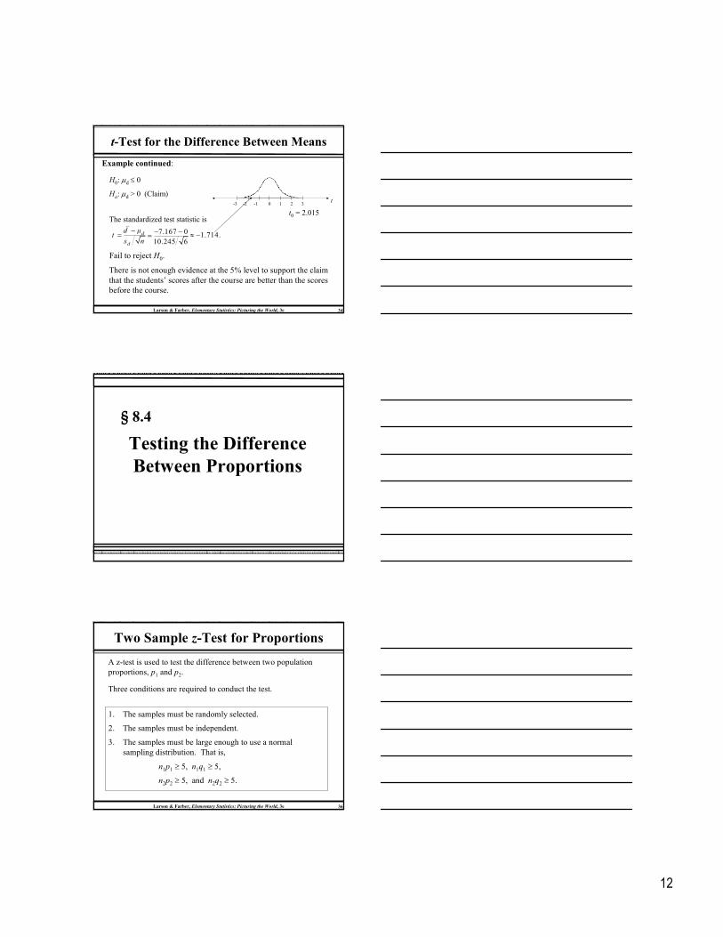
Two Sample z-Test for Proportions
A z-test is used to test the difference between two population
proportions, p1 and p2.
Three conditions are required to conduct the test.
1. The samples must be randomly selected.
2. The samples must be independent.
3. The samples must be large enough to use a normal
sampling distribution. That is,
n1p1 ≥ 5, n1q1 ≥ 5,
n2p2 ≥ 5, and n2q2 ≥ 5.
13
Larson & Farber, Elementary Statistics: Picturing the World, 3e 37
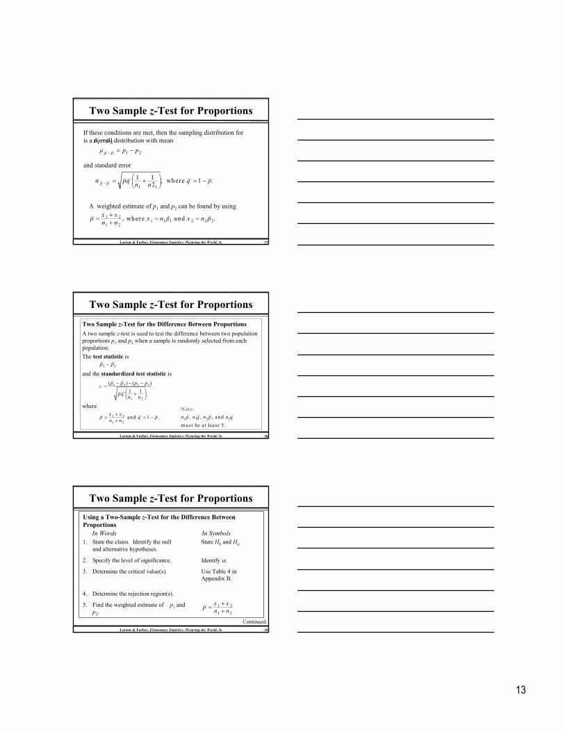
Two Sample z-Test for Proportions
If these conditions are met, then the sampling distribution for
is a normal distribution with mean1 2ˆ ˆp p−
1 21 2ˆ ˆp pµ p p− = −
and standard error
1 2ˆ ˆ
1 1
1 1, where 1 .
2p pσ pq q pn n− = + = −
A weighted estimate of p1 and p2 can be found by using
1 21 1 1 2 2 2
1 2
, where and .ˆ ˆx x
p x n p x n pn n
+= = =
+
Larson & Farber, Elementary Statistics: Picturing the World, 3e 38
Two Sample z-Test for Proportions
Two Sample z-Test for the Difference Between Proportions
A two sample z-test is used to test the difference between two population
proportions p1 and p2 when a sample is randomly selected from each
population.
The test statistic is
and the standardized test statistic is
where
1 2 1 2
1 2
( ) ( )ˆ ˆ
1 1
p p p pz
pqn n
− − −=
+
1 1ˆ ˆp p−
1 2
1 2
and 1 .x x
p q pn n
+= = −
+ 1 1 2 2, , , and
must b
Note:
e a t least 5.
n p n q n p n q
Larson & Farber, Elementary Statistics: Picturing the World, 3e 39
Two Sample z-Test for Proportions
1. State the claim. Identify the null
and alternative hypotheses.
2. Specify the level of significance.
3. Determine the critical value(s).
4. Determine the rejection region(s).
5. Find the weighted estimate of p1 and
p2.
Continued.
Using a Two-Sample z-Test for the Difference Between
Proportions
In Words In Symbols
State H0 and Ha.
Identify α.
Use Table 4 in
Appendix B.
1 2
1 2
x xp
n n
+=
+

14
Larson & Farber, Elementary Statistics: Picturing the World, 3e 40
Two Sample z-Test for Proportions
In Words In Symbols
6. Find the standardized test statistic.
7. Make a decision to reject or fail to reject
the null hypothesis.
8. Interpret the decision in the context of
the original claim.
Using a Two-Sample z-Test for the Difference Between
Proportions
1 2 1 2
1 2
( ) ( )ˆ ˆ
1 1
p p p pz
pqn n
− − −=
+
If z is in the rejection
region, reject H0.
Otherwise, fail to
reject H0.
Larson & Farber, Elementary Statistics: Picturing the World, 3e 41
Two Sample z-Test for Proportions
Example:
A recent survey stated that male college students smoke less than
female college students. In a survey of 1245 male students, 361
said they smoke at least one pack of cigarettes a day. In a survey of
1065 female students, 341 said they smoke at least one pack a day.
At α = 0.01, can you support the claim that the proportion of male
college students who smoke at least one pack of cigarettes a day is
lower then the proportion of female college students who smoke at
least one pack a day?
Ha: p1 < p2 (Claim)
H0: p1 ≥ p2
Continued.−z0 = −2.33
z0 1 2 3-3 -2 -1
α = 0.01
Larson & Farber, Elementary Statistics: Picturing the World, 3e 42
Two Sample z-Test for Proportions
Example continued:
Ha: p1 < p2 (Claim)
H0: p1 ≥ p2
Continued.
−z0 = −2.33
z0 1 2 3-3 -2 -1
1 2
1 2
x xp
n n
+=
+1 1 2 2
1 2
ˆ ˆn p n p
n n
+=
+361 341
1245 1065+=+
7022310
= 0.304≈
1 1 0.304 0.696q p= − = − =
Because 1245(0.304), 1245(0.696), 1065(0.304), and 1065(0.696) are all
at least 5, we can use a two-sample z-test.
15
Larson & Farber, Elementary Statistics: Picturing the World, 3e 43
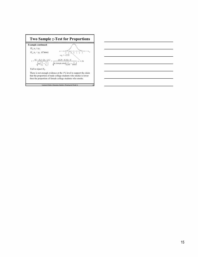
Two Sample z-Test for Proportions
Example continued:
Ha: p1 < p2 (Claim)
H0: p1 ≥ p2
−z0 = −2.33
z0 1 2 3-3 -2 -1
1 2 1 2
1 2
( ) ( )ˆ ˆ
1 1
p p p pz
pqn n
− − −=
+
( )(0.29 0.32) 0
1 1(0.304)(0.696)
1245 1065
− −=+
1.56≈ −
Fail to reject H0.
There is not enough evidence at the 1% level to support the claim
that the proportion of male college students who smoke is lower
then the proportion of female college students who smoke.