Chapter 8
99
Chapter 8 Profit Maximization and Competitive Supply
-
Upload
octavio-tyson -
Category
Documents
-
view
33 -
download
1
description
Chapter 8. Profit Maximization and Competitive Supply. Topics to be Discussed. Perfectly Competitive Markets Profit Maximization Marginal Revenue, Marginal Cost, and Profit Maximization Choosing Output in the Short-Run. Topics to be Discussed. The Competitive Firm’s Short-Run Supply Curve - PowerPoint PPT Presentation
Transcript of Chapter 8
Chapter 8Profit Maximization
and Competitive Supply
Profit Maximization and Competitive
Supply
Chapter 8 Slide 2
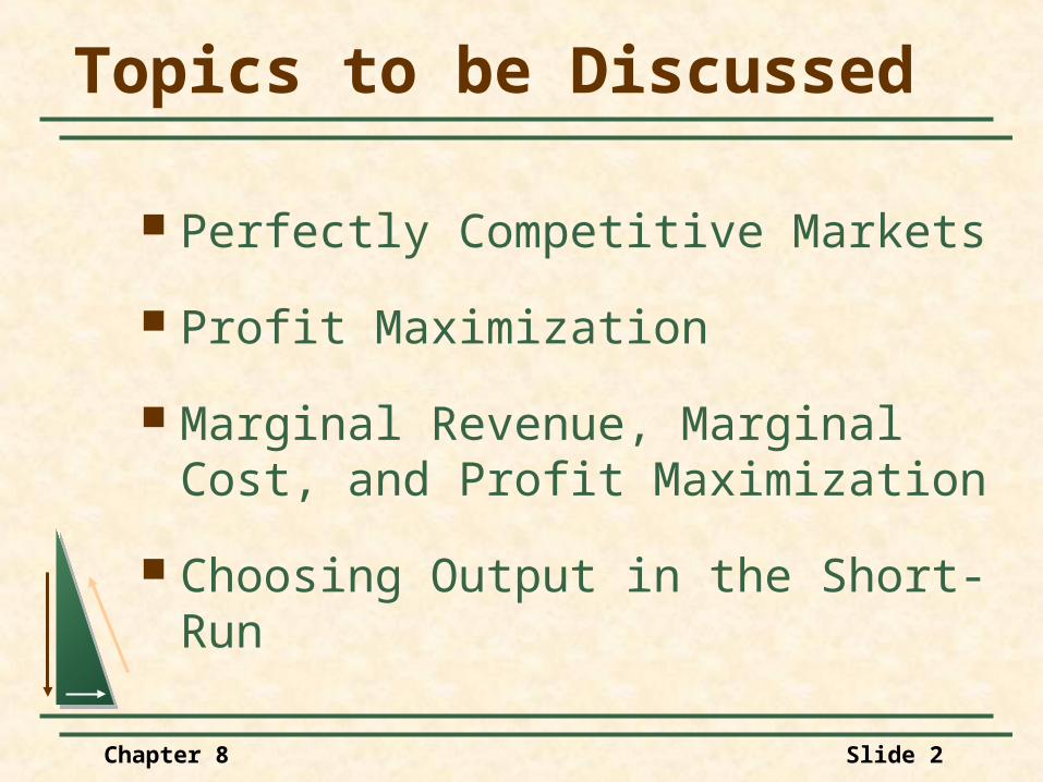
Topics to be Discussed
Perfectly Competitive Markets
Profit Maximization
Marginal Revenue, Marginal Cost, and Profit Maximization
Choosing Output in the Short-Run
Chapter 8 Slide 3
Topics to be Discussed
The Competitive Firm’s Short-Run Supply Curve
Short-Run Market Supply
Choosing Output in the Long-Run
The Industry’s Long-Run Supply Curve
Chapter 8 Slide 4
Perfectly Competitive Markets
Characteristics of Perfectly Competitive Markets
1) Price taking
2) Product homogeneity
3) Free entry and exit
Chapter 8 Slide 5
Perfectly Competitive Markets
Price Taking
The individual firm sells a very small share of the total market output and, therefore, cannot influence market price.
The individual consumer buys too small a share of industry output to have any impact on market price.
Chapter 8 Slide 6
Perfectly Competitive Markets
Product Homogeneity
The products of all firms are perfect substitutes.
Examples
Agricultural products, oil, copper, iron, lumber
Chapter 8 Slide 7
Perfectly Competitive Markets
Free Entry and Exit
Buyers can easily switch from one supplier to another.
Suppliers can easily enter or exit a market.
Chapter 8 Slide 8
Perfectly Competitive Markets
Discussion Questions
What are some barriers to entry and exit?
Are all markets competitive?
When is a market highly competitive?

Chapter 8 Slide 9
Profit Maximization
Do firms maximize profits?
Possibility of other objectivesRevenue maximizationDividend maximizationShort-run profit maximization

Chapter 8 Slide 10
Profit Maximization
Do firms maximize profits?
Implications of non-profit objectiveOver the long-run investors would not
support the companyWithout profits, survival unlikely
Chapter 8 Slide 11
Profit Maximization
Do firms maximize profits?
Long-run profit maximization is valid and does not exclude the possibility of altruistic behavior.

Chapter 8 Slide 12
Marginal Revenue, Marginal Cost,and Profit Maximization
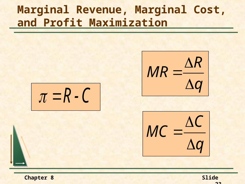
Determining the profit maximizing level of outputProfit ( ) = Total Revenue - Total Cost
Total Revenue (R) = Pq
Total Cost (C) = Cq
Therefore:
)()()( qCqRq
Chapter 8 Slide 13
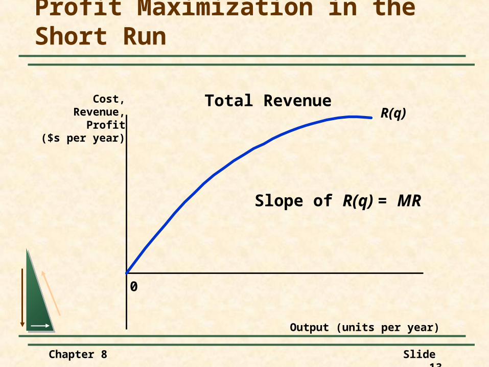
Profit Maximization in the Short Run
0
Cost,Revenue,
Profit($s per year)
Output (units per year)
R(q)Total Revenue
Slope of R(q) = MR
Chapter 8 Slide 14
0
Cost,Revenue,
Profit$ (per year)
Output (units per year)
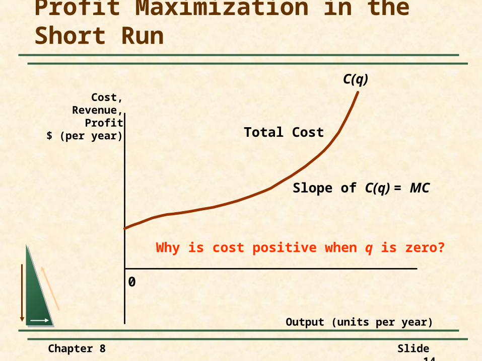
Profit Maximization in the Short Run
C(q)
Total Cost
Slope of C(q) = MC
Why is cost positive when q is zero?
Chapter 8 Slide 15
Marginal revenue is the additional revenue from producing one more unit of output.
Marginal cost is the additional cost from producing one more unit of output.
Marginal Revenue, Marginal Cost,and Profit Maximization

Chapter 8 Slide 16
Comparing R(q) and C(q)
Output levels: 0- q0:
C(q)> R(q) Negative profit
FC + VC > R(q) MR > MC
Indicates higher profit at higher output 0
Cost,Revenue,
Profit($s per year)
Output (units per year)
R(q)
C(q)
A
B
q0 q*
)(q
Marginal Revenue, Marginal Cost,and Profit Maximization

Chapter 8 Slide 17
Comparing R(q) and C(q) Question: Why is profit
negative when output is zero?
Marginal Revenue, Marginal Cost,and Profit Maximization
R(q)
0
Cost,Revenue,
Profit$ (per year)
Output (units per year)
C(q)
A
B
q0 q*
)(q

Chapter 8 Slide 18
Comparing R(q) and C(q)
Output levels: q0 - q*
R(q)> C(q) MR > MC
Indicates higher profit at higher output
Profit is increasing
R(q)
0
Cost,Revenue,
Profit$ (per year)
Output (units per year)
C(q)
A
B
q0 q*
)(q
Marginal Revenue, Marginal Cost,and Profit Maximization
Chapter 8 Slide 19
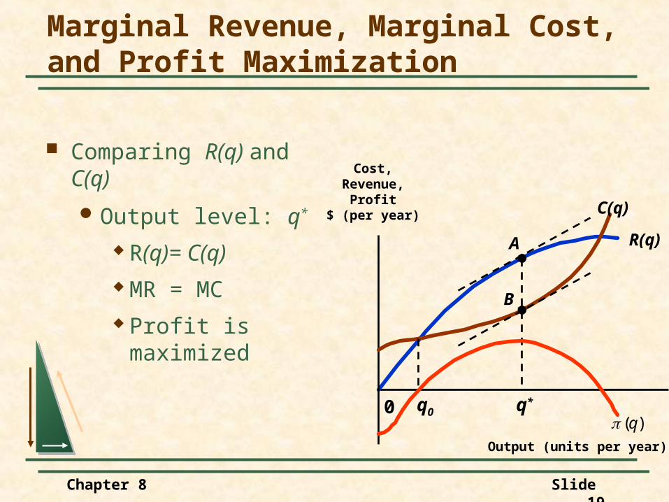
Comparing R(q) and C(q)
Output level: q*
R(q)= C(q) MR = MC Profit is maximized
R(q)
0
Cost,Revenue,
Profit$ (per year)
Output (units per year)
C(q)
A
B
q0 q*
)(q
Marginal Revenue, Marginal Cost,and Profit Maximization
Chapter 8 Slide 20
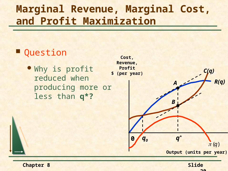
Question
Why is profit reduced when producing more or less than q*?
R(q)
0
Cost,Revenue,
Profit$ (per year)
Output (units per year)
C(q)
A
B
q0 q*
)(q
Marginal Revenue, Marginal Cost,and Profit Maximization

Chapter 8 Slide 21
Comparing R(q) and C(q)
Output levels beyond q*: R(q)> C(q) MC > MR Profit is decreasing
Marginal Revenue, Marginal Cost,and Profit Maximization
R(q)
0
Cost,Revenue,
Profit$ (per year)
Output (units per year)
C(q)
A
B
q0 q*
)(q
Chapter 8 Slide 22
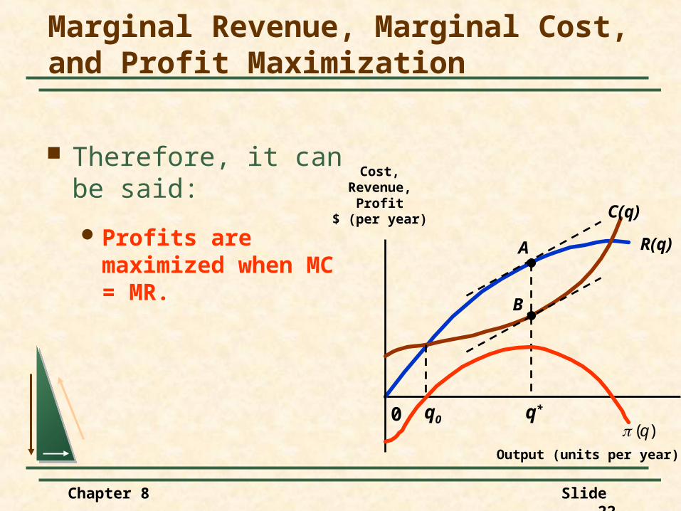
Therefore, it can be said:
Profits are maximized when MC = MR.
Marginal Revenue, Marginal Cost,and Profit Maximization
R(q)
0
Cost,Revenue,
Profit$ (per year)
Output (units per year)
C(q)
A
B
q0 q*
)(q
Chapter 8 Slide 23
C - R
Marginal Revenue, Marginal Cost,and Profit Maximization
q
R MR
q
CMC

Chapter 8 Slide 24
orq
C
q
R 0
q
: whenmaximized are Profits
MC(q)MR(q)
MCMR
thatso0
Marginal Revenue, Marginal Cost,and Profit Maximization

Chapter 8 Slide 25
The Competitive Firm
Price taker
Market output (Q) and firm output (q)
Market demand (D) and firm demand (d)
R(q) is a straight line
Marginal Revenue, Marginal Cost,and Profit Maximization
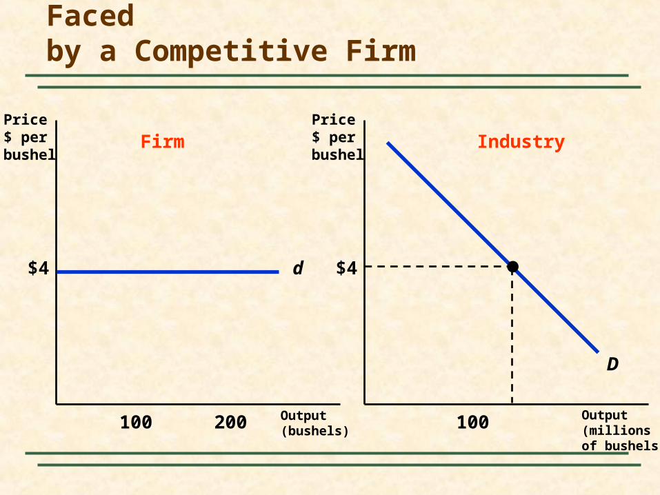
Demand and Marginal Revenue Facedby a Competitive Firm
Output (bushels)
Price$ per bushel
Price$ per bushel
Output (millions of bushels)
d$4
100 200 100
Firm Industry
D
$4
Chapter 8 Slide 27
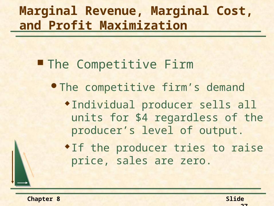
The Competitive Firm
The competitive firm’s demand Individual producer sells all units for $4
regardless of the producer’s level of output.
If the producer tries to raise price, sales are zero.
Marginal Revenue, Marginal Cost,and Profit Maximization
Chapter 8 Slide 28
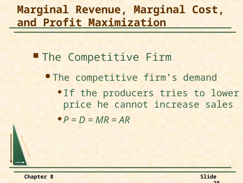
The Competitive Firm
The competitive firm’s demand If the producers tries to lower price he
cannot increase salesP = D = MR = AR
Marginal Revenue, Marginal Cost,and Profit Maximization

Chapter 8 Slide 29
The Competitive Firm
Profit MaximizationMC(q) = MR = P
Marginal Revenue, Marginal Cost,and Profit Maximization
Chapter 8 Slide 30
Choosing Output in the Short Run
We will combine production and cost analysis with demand to determine output and profitability.
Chapter 8 Slide 31
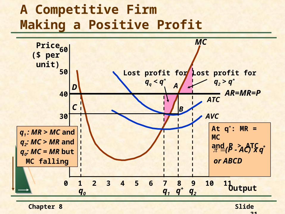
q0
Lost profit forqq < q*
Lost profit forq2 > q*
q1 q2
A Competitive FirmMaking a Positive Profit
10
20
30
40
Price($ per
unit)
0 1 2 3 4 5 6 7 8 9 10 11
50
60MC
AVC
ATCAR=MR=P
Outputq*
At q*: MR = MCand P > ATC
ABCDor
qx AC) -(P *
D A
BC
q1 : MR > MC andq2: MC > MR andq0: MC = MR but
MC falling

Chapter 8 Slide 32
Would this producercontinue to produce with a loss?
A Competitive FirmIncurring Losses
Price($ per
unit)
Output
AVC
ATCMC
q*
P = MR
B
F
C
A
E
DAt q*: MR = MCand P < ATCLosses = P- AC) x q* or ABCD
Chapter 8 Slide 33
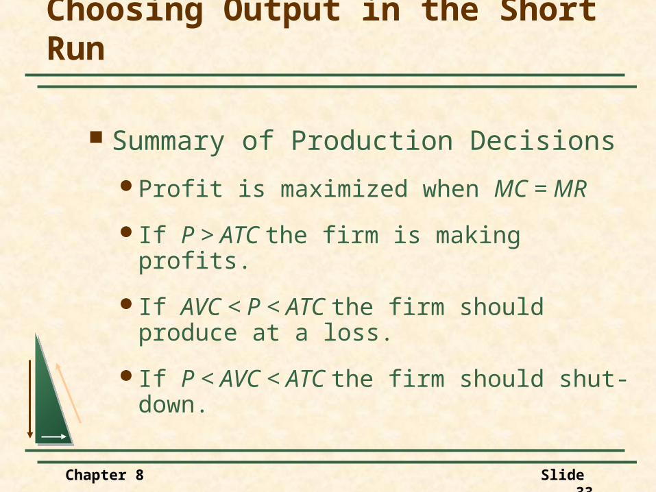
Choosing Output in the Short Run
Summary of Production Decisions
Profit is maximized when MC = MR
If P > ATC the firm is making profits.
If AVC < P < ATC the firm should produce at a loss.
If P < AVC < ATC the firm should shut-down.
Chapter 8 Slide 34
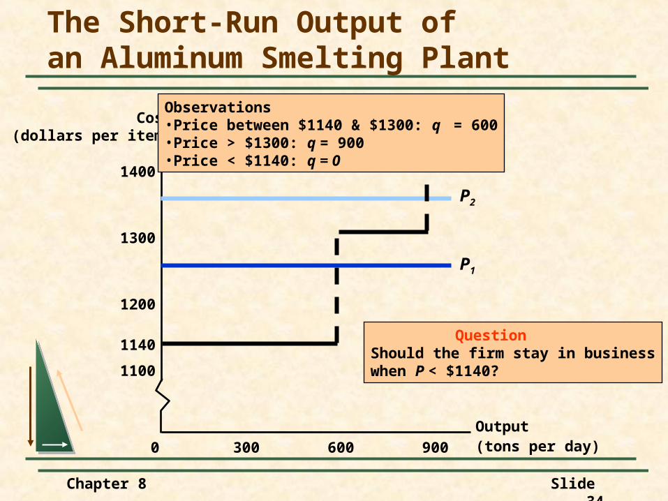
The Short-Run Output ofan Aluminum Smelting Plant
Output (tons per day)
Cost(dollars per item)
300 600 9000
1100
1200
1300
1400
1140
P1
P2
Observations•Price between $1140 & $1300: q = 600•Price > $1300: q = 900•Price < $1140: q = 0
QuestionShould the firm stay in businesswhen P < $1140?

Chapter 8 Slide 35
Some Cost Considerations for Managers
Three guidelines for estimating marginal cost:
1) Average variable cost should not be used as a substitute for marginal
cost.
Chapter 8 Slide 36
Some Cost Considerations for Managers
Three guidelines for estimating marginal cost:
2) A single item on a firm’s accounting ledger may have two components, only one of which involves marginal cost.

Chapter 8 Slide 37
Three guidelines for estimating marginal cost:
3) All opportunity cost should be included in determining
marginal cost.
Some Cost Considerations for Managers
Chapter 8 Slide 38
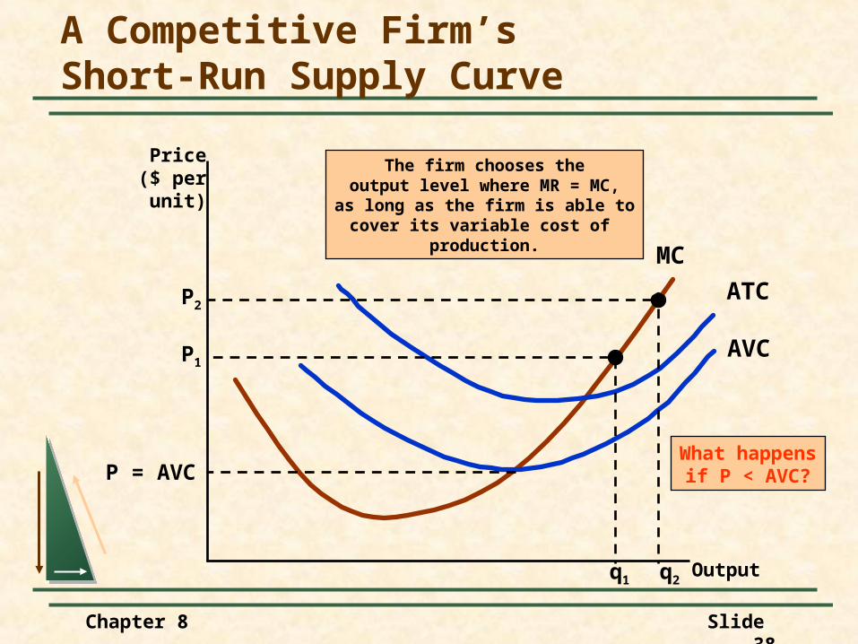
A Competitive Firm’sShort-Run Supply Curve
Price($ per
unit)
Output
MC
AVC
ATC
P = AVCWhat happens
if P < AVC?
P2
q2
P1
q1
The firm chooses theoutput level where MR = MC,as long as the firm is able to
cover its variable cost of production.

Chapter 8 Slide 39
Observations:P = MRMR = MCP = MC
Supply is the amount of output for every possible price. Therefore:If P = P1, then q = q1
If P = P2, then q = q2
A Competitive Firm’sShort-Run Supply Curve
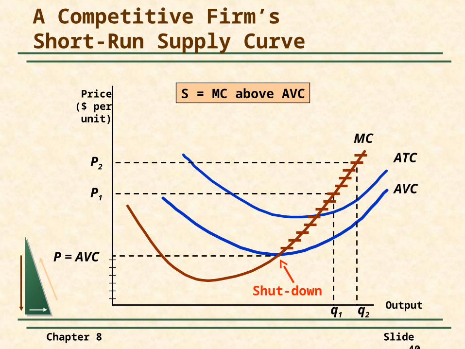
Chapter 8 Slide 40
Price($ per
unit)
MC
Output
AVC
ATC
P = AVC
P1
P2
q1 q2
S = MC above AVC
A Competitive Firm’sShort-Run Supply Curve
Shut-down
Chapter 8 Slide 41
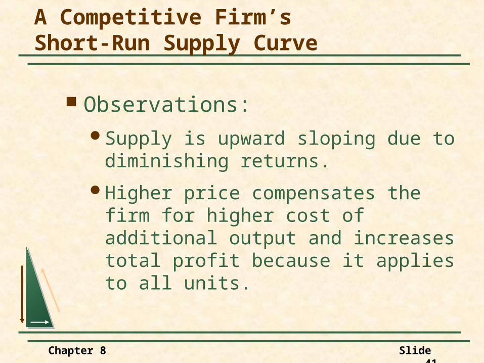
Observations:Supply is upward sloping due to
diminishing returns.
Higher price compensates the firm for higher cost of additional output and increases total profit because it applies to all units.
A Competitive Firm’sShort-Run Supply Curve

Chapter 8 Slide 42
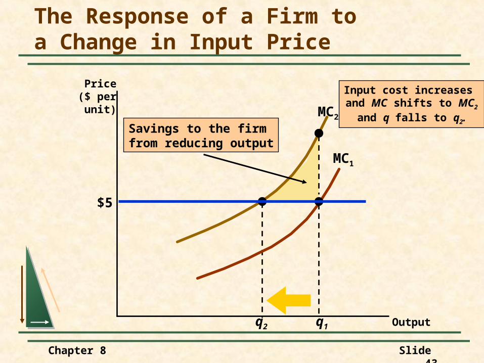
Firm’s Response to an Input Price ChangeWhen the price of a firm’s product
changes, the firm changes its output level, so that the marginal cost of production remains equal to the price.
A Competitive Firm’sShort-Run Supply Curve
Chapter 8 Slide 43
MC2
q2
Input cost increases and MC shifts to MC2
and q falls to q2.
MC1
q1
The Response of a Firm toa Change in Input Price
Price($ per
unit)
Output
$5
Savings to the firmfrom reducing output
Chapter 8 Slide 44
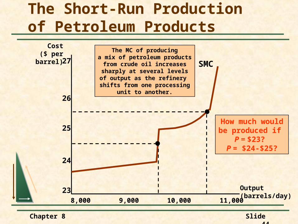
The Short-Run Productionof Petroleum Products
Cost($ per
barrel)
Output(barrels/day)
8,000 9,000 10,000 11,000
23
24
25
26
27 SMC
How much wouldbe produced if
P = $23? P = $24-$25?
The MC of producinga mix of petroleum products
from crude oil increasessharply at several levelsof output as the refinery
shifts from one processingunit to another.
Chapter 8 Slide 45
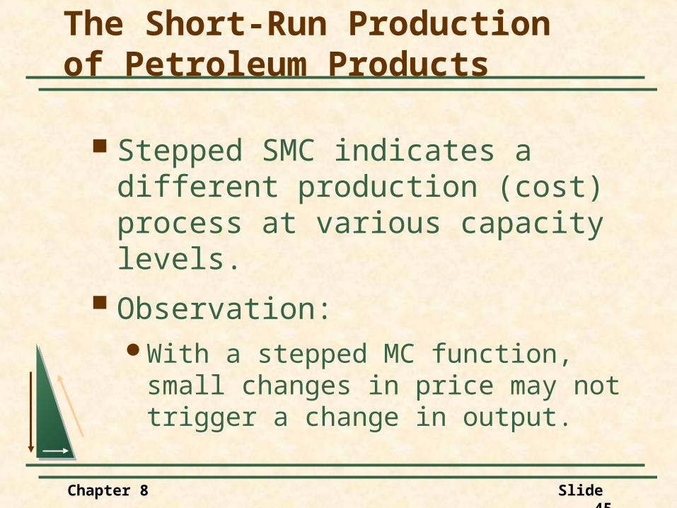
Stepped SMC indicates a different production (cost) process at various capacity levels.
Observation:With a stepped MC function, small
changes in price may not trigger a change in output.
The Short-Run Productionof Petroleum Products
Chapter 8 Slide 46
The short-run market supply curve shows the amount of output that the industry will produce in the short-run for every possible price.
Consider, for simplicity, a competitive market with three firms:
The Short-Run Productionof Petroleum Products
Chapter 8 Slide 47
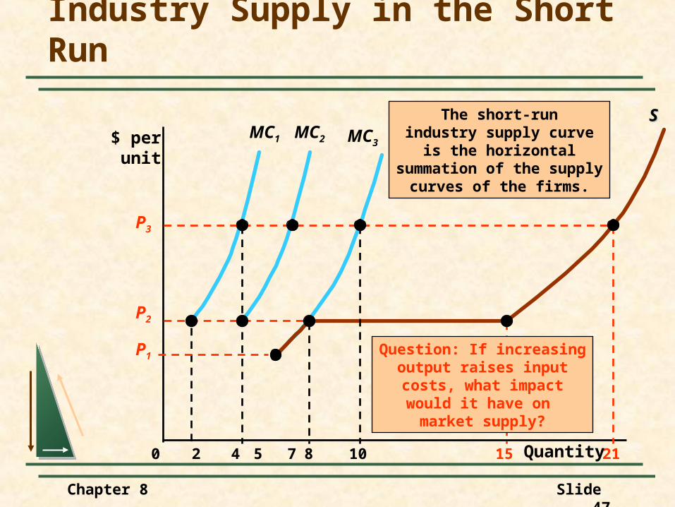
MC3
Industry Supply in the Short Run
$ perunit
0 2 4 8 105 7 15 21
MC1
SSThe short-runindustry supply curve
is the horizontalsummation of the supply
curves of the firms.
Quantity
MC2
P1
P3
P2
Question: If increasingoutput raises inputcosts, what impactwould it have on market supply?

Chapter 8 Slide 48
The Short-Run Market Supply Curve
Elasticity of Market Supply
)//()/( PPQQEs
Chapter 8 Slide 49
Perfectly inelastic short-run supply arises when the industry’s plant and equipment are so fully utilized that new plants must be built to achieve greater output.
Perfectly elastic short-run supply arises when marginal costs are constant.
The Short-Run Market Supply Curve
Chapter 8 Slide 50
Questions
1) Give an example of a perfectly inelastic supply.
2) If MC rises rapidly, would the supply be more or less elastic?
The Short-Run Market Supply Curve
Chapter 8 Slide 51
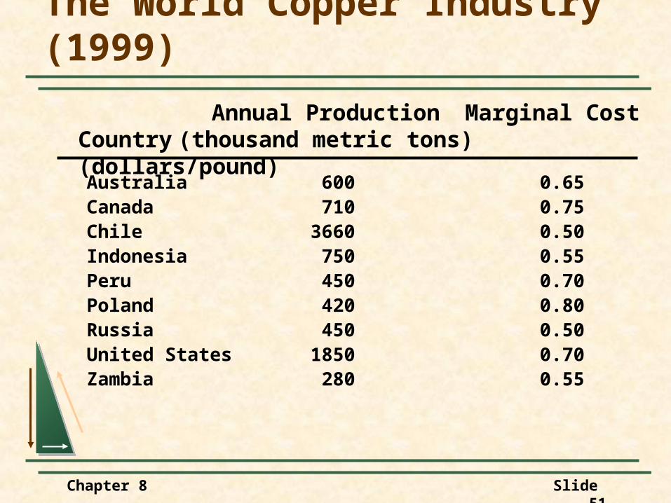
The World Copper Industry (1999)
Annual Production Marginal CostCountry (thousand metric tons) (dollars/pound)
Australia 600 0.65Canada 710 0.75Chile 3660 0.50Indonesia 750 0.55Peru 450 0.70Poland 420 0.80Russia 450 0.50United States 1850 0.70Zambia 280 0.55
Chapter 8 Slide 52
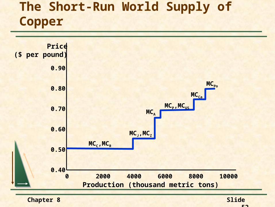
The Short-Run World Supply of Copper
Production (thousand metric tons)
Price($ per pound)
0 2000 4000 6000 8000 100000.40
0.50
0.60
0.70
0.80
0.90
MCC,MCR
MCJ,MCZ
MCA
MCP,MCUS
MCCa
MCPo
Chapter 8 Slide 53
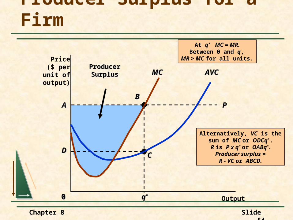
Producer Surplus in the Short RunFirms earn a surplus on all but the last unit
of output.
The producer surplus is the sum over all units produced of the difference between the market price of the good and the marginal cost of production.
The Short-Run Market Supply Curve
Chapter 8 Slide 54
AA
DD
BB
CC
ProducerProducerSurplusSurplus
Alternatively, VC is thesum of MC or ODCq* .R is P x q* or OABq*.Producer surplus =
R - VC or ABCD.
Producer Surplus for a Firm
Price($ per
unit ofoutput)
Output
AVCAVCMCMC
00
PP
qq**
At q* MC = MR.Between 0 and q ,
MR > MC for all units.
Chapter 8 Slide 55
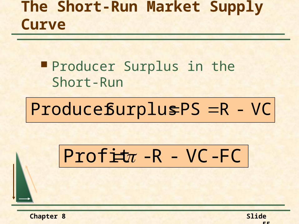
Producer Surplus in the Short-Run
The Short-Run Market Supply Curve
VC- R PS Surplus Producer
FC - VC- R - Profit
Chapter 8 Slide 56
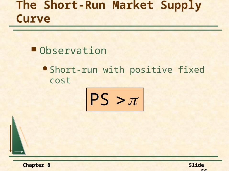
Observation
Short-run with positive fixed cost
The Short-Run Market Supply Curve
PS
Chapter 8 Slide 57
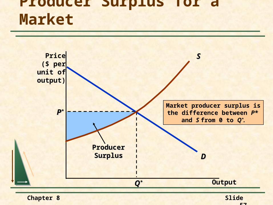
DD
PP**
QQ**
ProducerProducerSurplusSurplus
Market producer surplus isthe difference between P*
and S from 0 to Q*.
Producer Surplus for a Market
Price($ per
unit ofoutput)
Output
SS
Chapter 8 Slide 58
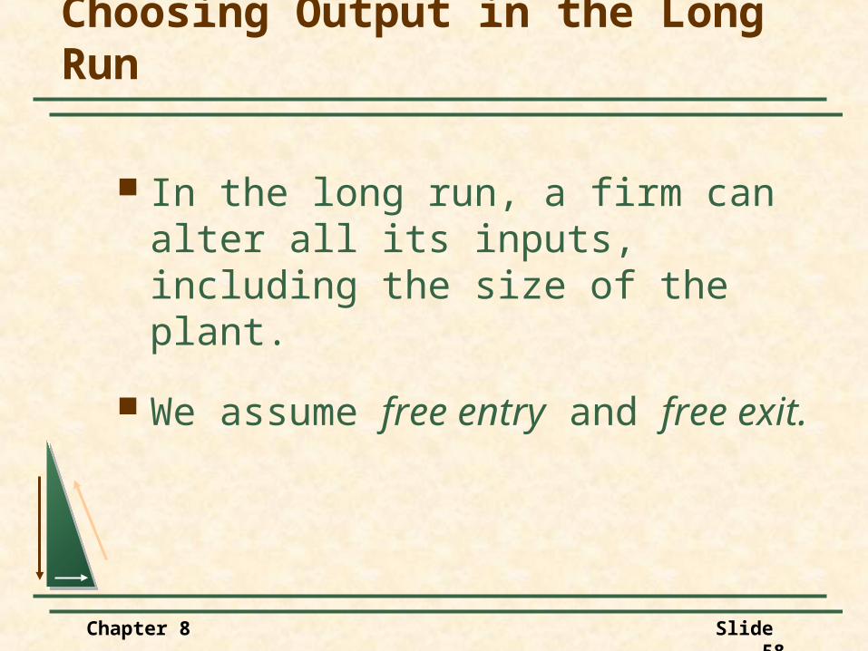
Choosing Output in the Long Run
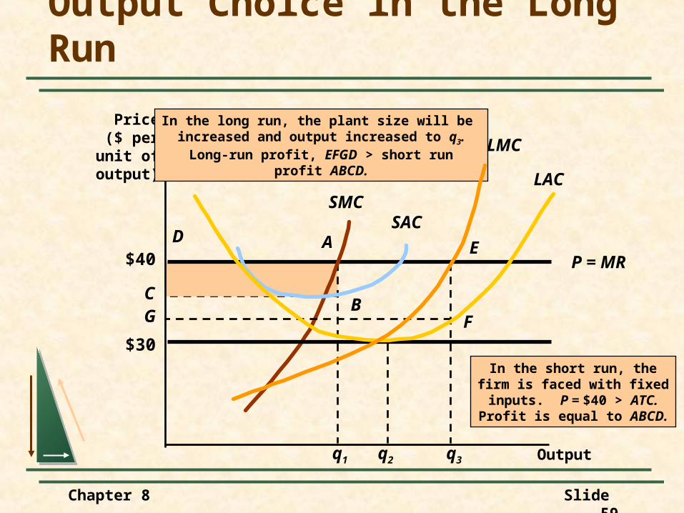
In the long run, a firm can alter all its inputs, including the size of the plant.
We assume free entry and free exit.
Chapter 8 Slide 59
q1
A
BC
D
In the short run, thefirm is faced with fixedinputs. P = $40 > ATC.Profit is equal to ABCD.
Output Choice in the Long Run
Price($ per
unit ofoutput)
Output
P = MR$40
SACSMC
In the long run, the plant size will be increased and output increased to q3.
Long-run profit, EFGD > short runprofit ABCD.
q3q2
G F$30
LAC
E
LMC
Chapter 8 Slide 60
q1
A
BC
D
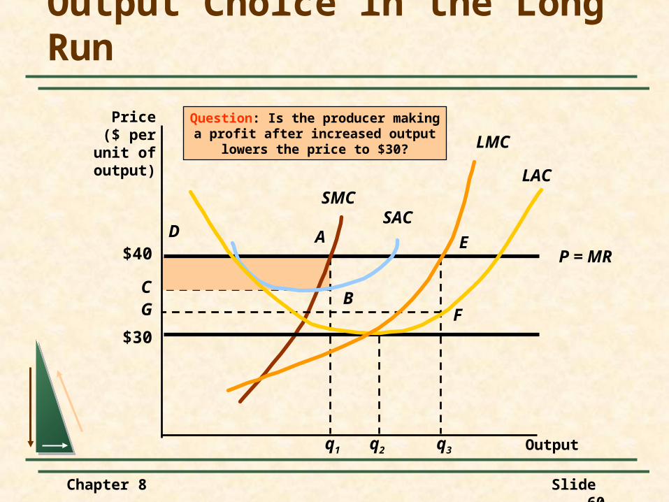
Output Choice in the Long Run
Price($ per
unit ofoutput)
Output
P = MR$40
SACSMC
Question: Is the producer makinga profit after increased output
lowers the price to $30?
q3q2
G F$30
LAC
E
LMC

Chapter 8 Slide 61
Choosing Output in the Long Run
Accounting Profit & Economic ProfitAccounting profit = R - wL
Economic profit = R = wL - rKwl = labor cost
rk = opportunity cost of capital
)()(
Chapter 8 Slide 62
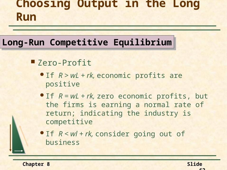
Choosing Output in the Long Run
Zero-ProfitIf R > wL + rk, economic profits are positive
If R = wL + rk, zero economic profits, but the firms is earning a normal rate of return; indicating the industry is competitive
If R < wl + rk, consider going out of business
Long-Run Competitive EquilibriumLong-Run Competitive Equilibrium

Chapter 8 Slide 63
Choosing Output in the Long Run
Entry and ExitThe long-run response to short-run profits
is to increase output and profits.
Profits will attract other producers.
More producers increase industry supply which lowers the market price.
Long-Run Competitive EquilibriumLong-Run Competitive Equilibrium

S1
Long-Run Competitive Equilibrium
Output Output
$ per unit ofoutput
$ per unit ofoutput
$40LAC
LMC
D
S2
P1
Q1q2
Firm Industry
$30
Q2
P2
•Profit attracts firms•Supply increases until profit = 0

Chapter 8 Slide 65
Choosing Output in the Long Run
Long-Run Competitive Equilibrium
1) MC = MR
2) P = LAC
No incentive to leave or enter
Profit = 0
3) Equilibrium Market Price
Chapter 8 Slide 66
Choosing Output in the Long Run
Questions
1) Explain the market adjustment when P < LAC and firms have identical costs.
2) Explain the market adjustment when firms have different costs.
3) What is the opportunity cost of land?

Chapter 8 Slide 67
Choosing Output in the Long Run
Economic RentEconomic rent is the difference between
what firms are willing to pay for an input less the minimum amount necessary to obtain it.

Chapter 8 Slide 68
Choosing Output in the Long Run
An Example
Two firms A & B
Both own their land
A is located on a river which lowers A’s shipping cost by $10,000 compared to B.
The demand for A’s river location will increase the price of A’s land to $10,000
Chapter 8 Slide 69
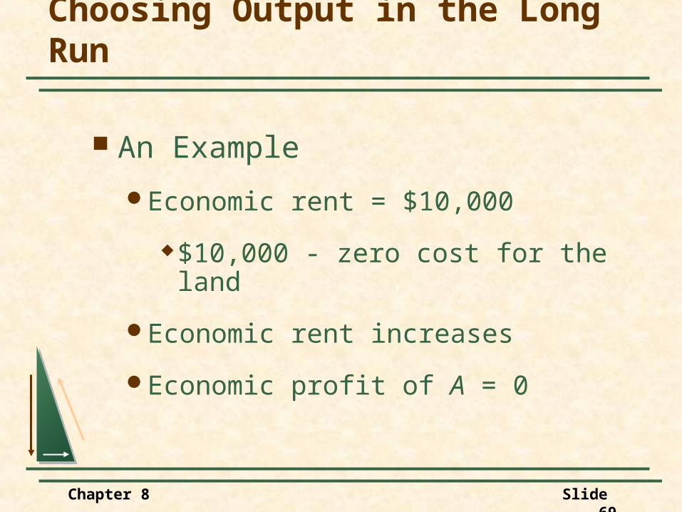
Choosing Output in the Long Run
An Example
Economic rent = $10,000
$10,000 - zero cost for the land
Economic rent increases
Economic profit of A = 0

Chapter 8 Slide 70
Firms Earn Zero Profit inLong-Run Equilibrium
TicketPrice
Season TicketsSales (millions)
LAC
$7$7
1.01.0
A baseball teamin a moderate-sized city
sells enough tickets so that price is equal to marginal
and average cost(profit = 0).
LMC
Chapter 8 Slide 71
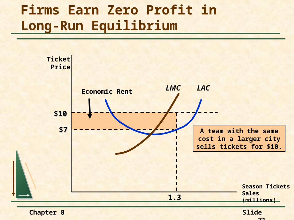
1.31.3
$10$10
Economic Rent
TicketPrice
$7$7
LAC
A team with the samecost in a larger citysells tickets for $10.
Firms Earn Zero Profit inLong-Run Equilibrium
Season TicketsSales (millions)
LMC

Chapter 8 Slide 72
With a fixed input such as a unique location, the difference between the cost of production (LAC = 7) and price ($10) is the value or opportunity cost of the input (location) and represents the economic rent from the input.
Firms Earn Zero Profit inLong-Run Equilibrium
Chapter 8 Slide 73
If the opportunity cost of the input (rent) is not taken into consideration it may appear that economic profits exist in the long-run.
Firms Earn Zero Profit inLong-Run Equilibrium

Chapter 8 Slide 74
The shape of the long-run supply curve depends on the extent to which changes in industry output affect the prices the firms must pay for inputs.
The Industry’s Long-Run Supply Curve
Chapter 8 Slide 75
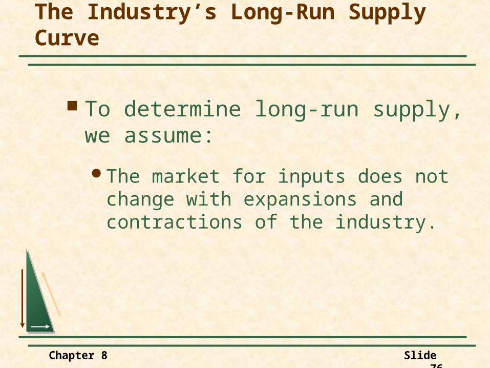
The Industry’s Long-Run Supply Curve
To determine long-run supply, we assume:
All firms have access to the available production technology.
Output is increased by using more inputs, not by invention.
Chapter 8 Slide 76
The Industry’s Long-Run Supply Curve
To determine long-run supply, we assume:
The market for inputs does not change with expansions and contractions of the industry.

AP1
AC
P1
MC
q1
D1
S1
Q1
C
D2
P2P2
q2
B
S2
Q2
Economic profits attract newfirms. Supply increases to S2 and
the market returns to long-run equilibrium.
Long-Run Supply in aConstant-Cost Industry
Output Output
$ per unit ofoutput
$ per unit ofoutput
SL
Q1 increase to Q2.Long-run supply = SL = LRAC.
Change in output has no impact on input cost.

Chapter 8 Slide 78
In a constant-cost industry, long-run supply is a horizontal line at a price that is equal to the minimum average cost of production.
Long-Run Supply in aConstant-Cost Industry
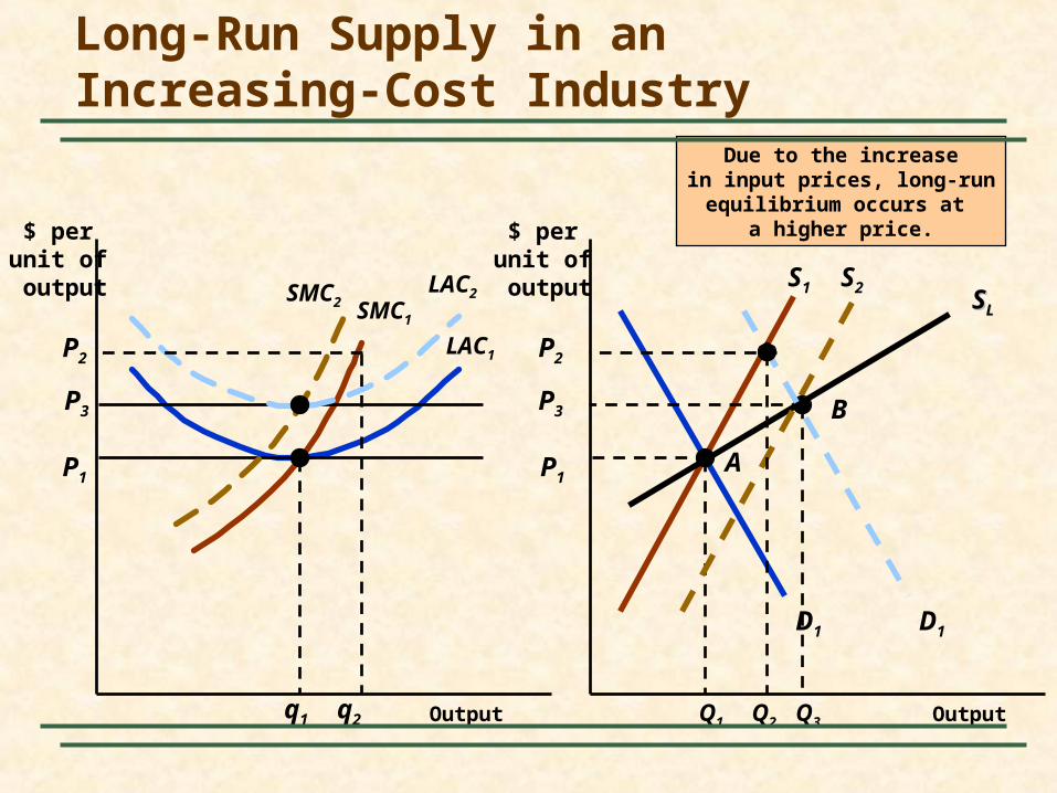
Long-Run Supply in anIncreasing-Cost Industry
Output Output
$ per unit ofoutput
$ per unit ofoutput S1
D1
P1
LAC1
P1
SMC1
q1 Q1
A
SSLL
P3
SMC2
Due to the increasein input prices, long-runequilibrium occurs at
a higher price.
LAC2
B
S2
P3
Q3q2
P2 P2
D1
Q2

Chapter 8 Slide 80
In a increasing-cost industry, long-run supply curve is upward sloping.
Long-Run Supply in aIncreasing-Cost Industry
Chapter 8 Slide 81
The Industry’sLong-Run Supply Curve
Questions
1) Explain how decreasing-cost is possible.
2) Illustrate a decreasing cost industry.
3) What is the slope of the SL in a decreasing-cost industry?

S2
B
SL
P3
Q3
SMC2
P3
LAC2
Due to the decreasein input prices, long-runequilibrium occurs at
a lower price.
Long-Run Supply in anDecreasing-Cost Industry
Output Output
$ per unit ofoutput
$ per unit ofoutput
P1P1
SMC1
A
D1
S1
Q1q1
LAC1
Q2q2
P2 P2
D2
Chapter 8 Slide 83
In a decreasing-cost industry, long-run supply curve is downward sloping.
Long-Run Supply in aIncreasing-Cost Industry
Chapter 8 Slide 84
The Effects of a TaxIn an earlier chapter we studied how firms
respond to taxes on an input.
Now, we will consider how a firm responds to a tax on its output.
The Industry’sLong-Run Supply Curve
Chapter 8 Slide 85
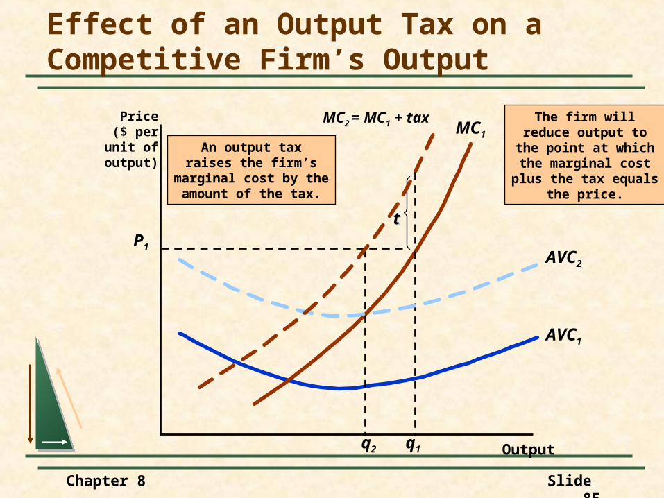
Effect of an Output Tax on a Competitive Firm’s Output
Price($ per
unit ofoutput)
Output
AVC1
MC1
P1
q1
The firm willreduce output to
the point at whichthe marginal cost
plus the tax equalsthe price.
q2
tt
MC2 = MC1 + tax
AVC2
An output taxraises the firm’s
marginal cost by theamount of the tax.

Chapter 8 Slide 86
Effect of an OutputTax on Industry Output
Price($ per
unit ofoutput)
Output
DD
P1
SS1
Q1
P2
Q2
SS2 = S1 + t
t
Tax shifts S1 to S2 andoutput falls to Q2. Price
increases to P2.

Chapter 8 Slide 87
Long-Run Elasticity of Supply
1) Constant-cost industryLong-run supply is horizontalSmall increase in price will induce an
extremely large output increase
The Industry’sLong-Run Supply Curve
Chapter 8 Slide 88
Long-Run Elasticity of Supply
1) Constant-cost industryLong-run supply elasticity is infinitely
large Inputs would be readily available
The Industry’sLong-Run Supply Curve
Chapter 8 Slide 89
Long-Run Elasticity of Supply
2) Increasing-cost industryLong-run supply is upward-sloping and
elasticity is positiveThe slope (elasticity) will depend on the
rate of increase in input costLong-run elasticity will generally be
greater than short-run elasticity of supply
The Industry’sLong-Run Supply Curve

Chapter 8 Slide 90
Question:Describe the long-run elasticity of supply in
a decreasing -cost industry.
The Industry’sLong-Run Supply Curve

Chapter 8 Slide 91
The Long-Run Supply of Housing
Scenario 1: Owner-occupied housingSuburban or rural areas
National market for inputs
Chapter 8 Slide 92
The Long-Run Supply of Housing
QuestionsIs this an increasing or a constant-cost
industry?
What would you predict about the elasticity of supply?

Chapter 8 Slide 93
Scenario 2: Rental propertyZoning restrictions applyUrban locationHigh-rise construction cost
The Long-Run Supply of Housing
Chapter 8 Slide 94
QuestionsIs this an increasing or a constant-cost
industry?What would you predict about the elasticity
of supply?
The Long-Run Supply of Housing
Chapter 8 Slide 95
Summary
The managers of firms can operate in accordance with a complex set of objectives and under various constraints.
A competitive market makes its output choice under the assumption that the demand for its own output is horizontal.
Chapter 8 Slide 96
Summary
In the short run, a competitive firm maximizes its profit by choosing an output at which price is equal to (short-run) marginal cost.
The short-run market supply curve is the horizontal summation of the supply curves of the firms in an industry.

Chapter 8 Slide 97
Summary
The producer surplus for a firm is the difference between revenue of a firm and the minimum cost that would be necessary to produce the profit-maximizing output.
Economic rent is the payment for a scarce resource of production less the minimum amount necessary to hire that factor.
Chapter 8 Slide 98
Summary
In the long-run, profit-maximizing competitive firms choose the output at which price is equal to long-run marginal cost.
The long-run supply curve for a firm can be horizontal, upward sloping, or downward sloping.

End of Chapter 8Profit Maximization
and Competitive Supply
Profit Maximization and Competitive
Supply