Chapter 8 © 2006 Thomson Learning/South-Western Costs.

Chapter 8Chapter 8

© 2006 Thomson Learning/South-Western

Costs

2

Basic Concepts of Costs

Opportunity cost: the cost of a good or service as measured by the alternative uses that are foregone by producing the good or service.

Accounting cost: the concept that goods or services cost what was paid for them.

Economic cost: the amount required to keep a resource in its present use; the amount that it would be worth in its next best alternative use.

3

Labor Costs

Like accountants, economists regard the payments to labor as an explicit cost.

Labor services (worker-hours) are purchased at an hourly wage rate (w): The cost of hiring one worker for one hour.

The wage rate is assumed to be the amount workers would receive in their next best alternative employment.

4

Capital Costs

Economists consider the cost of a machine to be the amount someone else would be willing to pay for its use.

The cost of capital services (machine-hours) is the rental rate (v) which is the cost of hiring one machine for one hour.

This is an implicit cost if the machine is owned by the firm.

5

Entrepreneurial Costs

Owners of the firm are entitled to the difference between revenue and costs which is generally called (accounting) profit.

Economic profit is revenue minus all costs including these entrepreneurial costs.

6

The Two-Input Case

The firm uses only two inputs: labor (L, measured in labor hours) and capital (K, measured in machine hours). Entrepreneurial services are assumed to be

included in the capital costs. Firms buy inputs in perfectly competitive

markets so the firm faces horizontal supply curves at prevailing factor prices.

7

Economic Profits and Cost Minimization

Total costs = TC = wL + vK. (8.1) Assuming the firm produces only one

output, total revenue equals the price of the product (P) times its total output [q = f(K,L) where f(K,L) is the firm’s production function].

8

Economic Profits and Cost Minimization

Economic profits (): the difference between a firm’s total revenues and its total economic costs.

.),(

2.8

vKwLLKPf

vKwLPq

costs Total - revenues Total

9

Graphic Presentation

The isoquant q1 shows all combinations of K and L that are required to produce q1.

The slope of total costs, TC = wL + vK, is -w/v.

Lines of equal cost will have the same slope so they will be parallel.

Three equal total costs lines, labeled TC1, TC2, and TC3 are shown in Figure 8-1.

10

Capitalper week

TC1

TC2

TC3

q1

K*

Laborper weekL*0

FIGURE 8-1: Minimizing the Costs of Producing q1

11

Graphic Presentation

The minimum total cost of producing q1 is TC1 (since it is closest to the origin).

The cost-minimizing input combination is L*, K* which occurs where the total cost curve is tangent to the isoquant.

At the point of tangency, the rate at which the firm can technically substitute L for K (the RTS) equals the market rate (w/v).

12

Cost-Minimizing Input Choice

Cost minimization requires that the marginal rate of technical substitution (RTS) of L for K equals the ratio of the inputs’ costs, w/v:

3.8(K

L

MP

MPRTS K) for L

13

An Alternative Interpretation

5.8.

4.8,)(

.(

v

MP

w

MP

v

w

MP

MPKforLRTS

MP

MPRTS

KL

K

L

K

L

K) for L

From Chapter 7

Cost minimization requires

or, rearranging

14

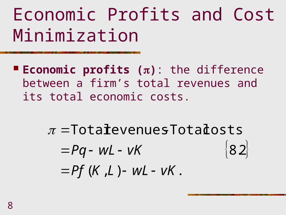
The Firm’s Expansion Path

A similar analysis could be performed for any output level (q).

If input costs (w and v) remain constant, various cost-minimizing choices can be traces out as shown in Figure 8-2.

For example, output level q1 is produced using K1, L1, and other cost-minimizing points are shown by the tangency between the total cost lines and the isoquants.

15

The Firm’s Expansion Path

The firm’s expansion path is the set of cost-minimizing input combinations a firm will choose to produce various levels of output (when the prices of inputs are held constant).

Although in Figure 8-2, the expansion path is a straight line, that is not necessarily the case.

16

Capitalper week

TC1 TC3TC2 Expansion path

q1

q2

q3

K1

Laborper weekL10

FIGURE 8-2: Firm’s Expansion Path

17

Cost Curves

Figure 8-3 shows four possible shapes for cost curves.

In Panel a, output and required input use is proportional which means doubling of output requires doubling of inputs. This is the case when the production function exhibits constant returns to scale.

18

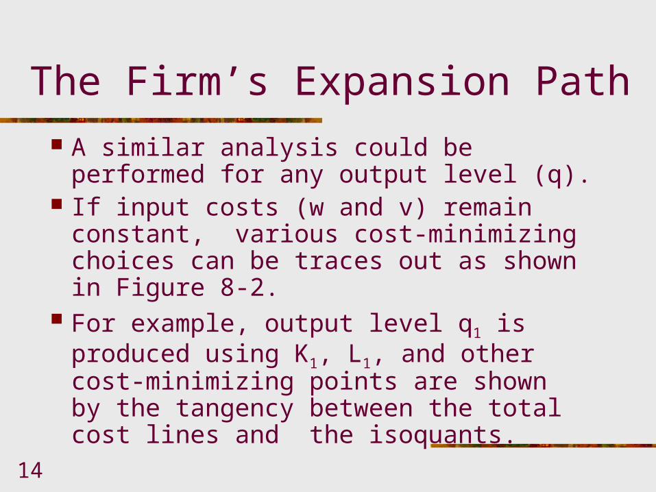
Cost Curves Panels b and c reflect the cases of decreasing

and increasing returns to scale, respectively. With decreasing returns to scale the cost curve is

convex, while it is concave with increasing returns to scale.

Decreasing returns to scale indicate considerable cost advantages from large scale operations.

Panel d reflects the case where there are increasing returns to scale followed by decreasing returns to scale.

19

Totalcost

TC

Quantityper week

(a) Constant Returns to Scale

0

Totalcost

TC

Quantityper week

(b) Decreasing Returns to Scale

0

Totalcost TC

Quantityper week

(c) Increasing Returns to Scale

0

Totalcost

TC

Quantityper week

(d) Optimal Scale

0

FIGURE 8-3: Possible Shapes of the Total Cost Curve

20

Average Costs

Average cost is total cost divided by output; a common measure of cost per unit.

If the total cost of producing 25 units is $100, the average cost would be

6.8q

TCAC cost Average

4$25

100$AC

21

Marginal Cost

The additional cost of producing one more unit of output is marginal cost.

If the cost of producing 24 units is $98 and the cost of producing 25 units is $100, the marginal cost of the 25th unit is $2.

7.8q in Change

TC in Changecost Marginal MC

22

Marginal Cost Curves

Marginal costs are reflected by the slope of the total cost curve.

The constant returns to scale total cost curve shown in Panel a of Figure 8-3 has a constant slope, so the marginal cost is constant as shown by the horizontal marginal cost curve in Panel a of Figure 8-4.

23

AC, MC

AC, MC

Quantityper week


0

FIGURE 8-4: Average and Marginal Cost Curves

24


With decreasing returns to scale, the total cost curve is convex (Panel b of Figure 8-3).

This means that marginal costs are increasing which is shown by the positively sloped marginal cost curve in Panel b of Figure 8-4.

25

AC, MC

AC, MC

Quantityper week


0

AC, MCAC

MC

Quantityper week


0


26


Increasing returns to scale results in a concave total cost curve (Panel c of Figure 8-3).

This causes the marginal costs to decrease as output increases as shown in the negatively sloped marginal cost curve in Panel c of Figure 8-4.

27

AC, MC

AC, MC

Quantityper week


0

AC, MCAC

AC

MC

MC

Quantityper week


0

AC, MC

Quantityper week


0


28


When the total cost curve is first concave followed by convex as shown in Panel d of Figure 8-3, marginal costs initially decrease but eventually increase.

Thus, the marginal cost curve is first negatively sloped followed by a positively sloped curve as shown in Panel d of Figure 8-4.

29

AC, MC

AC, MC

Quantityper week


0

AC, MCAC

AC

AC

MC

MC

MC

Quantityper week


0

AC, MC

Quantityper week


0

AC, MC

Quantityper week

(d) Optimal Scale

0 q*


30

Average Cost Curves

For the constant returns to scale case, marginal cost never varies from its initial level, so average cost must stay the same as well.

Thus, the average cost curve are the same horizontal line as shown in Panel a of Figure 8-4.

31

Average Cost Curves

With convex total costs and increasing marginal costs, average costs also rise as shown in Panel b of Figure 8-4.

Because the first few units are produced at low marginal costs, average costs will always be less than marginal cost, so the average cost curve lies below the marginal cost curve.

32

Average Cost Curves

With concave total cost and decreasing marginal costs, average costs will also decrease as shown in Panel c in Figure 8-4.

Because the first few units are produced at relatively high marginal costs, average is less than marginal cost, so the average cost curve lies below the marginal cost curve.

33

Average Cost Curves

The U-shaped marginal cost curve shown in Panel d of Figure 8-4 reflects decreasing marginal costs at low levels of output and increasing marginal costs at high levels of output.

As long as marginal cost is below average cost, the marginal will pull down the average.

34

Average Cost Curves

When marginal costs are above average cost, the marginal pulls up the average.

Thus, the average cost curve must intersect the marginal cost curve at the minimum average cost; q* in Panel d of Figure 8-4.

Since q* represents the lowest average cost, it represents an “optimal scale” of production for the firm.

35

Input Inflexibility and Cost Minimization

Since capital is fixed, short-run costs are not the minimal costs of producing variable output levels.

Assume the firm has fixed capital of K1 as shown in Figure 8-5.

To produce q0 of output, the firm must use L1 units of labor, with similar situations for q1, L1, and q2, L2.

36

Capitalper week

STC0 STC2STC1

q1

q2

q0

K1

Laborper weekL0 L1 L20

FIGURE 8-5: “Nonoptimal” Input Choices Must Be Made in the Short Run

37

Input Inflexibility and Cost Minimization

The cost of output produced is minimized where the RTS equals the ratio of prices, which only occurs at q1, L1.

Q0 could be produce at less cost if less capital than K1 and more labor than L0 were used.

Q2 could be produced at less cost if more capital than K1 and less labor than L2 were used.

38

Per-Unit Short-Run Cost Curves

q in Change

STC in Changecost marginal run-Short

and

cost average run-Short

SMC

q

STCSAC

39

Per-Unit Short-Run Cost Curves

Having capital fixed in the short run yields a total cost curve that has both concave and convex sections, the resulting short-run average and marginal cost relationships will also be U-shaped.

When SMC < SAC, average cost is falling, but when SMC > SAC average cost increase.

40

SMC

MC

SAC

AC

AC, MC

Quantityper week

0 q*

FIGURE 8-6: Short-Run and Long-Run Average and Marginal Cost Curves at Optimal Output Level

41

Relationship between Short-Run and Long-Run per-Unit Cost Curves

In the short-run, when the firm using K* units of capital produces q*, short-run and long-run total costs are equal.

In addition, as shown in Figure 8-6 AC = MC = SAC(K*) = SMC(K*).

(8.8) For output above q* short-run costs are

higher than long-run costs. The higher per-unit costs reflect the facts that K is fixed.

42

Shifts in Cost Curves

Any change in economic conditions that affects the expansion path will also affect the shape and position of the firm’s cost curves.

Three sources of such change are: change in input prices technological innovations, and economies of scope.

43

TABLE 8-1: Total Costs of Producing 40 Hamburgers per Hour

Output (q) Workers (L) Grills (K) Total Cost (TC) 40 1 16.0 $85.00 40 2 8.0 50.00 40 3 5.3 41.50 40 4 4.0 40.00 40 5 3.2 41.00 40 6 2.7 43.50 40 7 2.3 46.50 40 8 2.0 50.00 40 9 1.8 54.00 40 10 1.6 58.00

44

Grillsper hour

2

8

4

Workersper hour

40 hamburgers per hour

E

Total cost = $40

2 4 80

Figure 8-7: Cost-Minimizing Input Choice for 40 Hamburgers per Hour

45

Long-Run cost Curves

HH’s production function is constant returns to scale so

As long as w = v = $5, all of the cost minimizing tangencies will resemble the one shown in Figure 8.7 and long-run cost minimization will require K = L.

46

Long-Run cost Curves

This situation, resulting from constant returns to scale, is shown in Figure 8-8.

HH’s long-run total cost function is a straight line through the origin as shown in Panel a.

Its long-run average and marginal costs are constant at $1 per burger as shown in Panel b.

47

Totalcosts

20

60

$80

40

Totalcosts

40 6020 80

(a) Total Costs

0

Average andmarginal costs

$1.00

Hamburgersper hour

40 6020 80

(b) Average and Marginal Costs

0

FIGURE 8-8: Total, Average, and Marginal Cost Curves


Hamburgersper hour

48

Short-Run Costs

Table 8-2 repeats the labor input required to produce various output levels holding grills fixed at 4.

Diminishing marginal productivity of labor causes costs to rise rapidly as output expands.

Figure 8-9 shows the short-run average and marginal costs curves.

49

TABLE 8-2: Short-Run Costs of Hamburger Production

Output (q) Workers

(L) Grills (K)

Total Cost (STC)

Average Cost (SAC)

Marginal Cost (SMC)

10 0.25 4 $21.25 $2.125 - 20 1.00 4 25.00 1.250 $0.50 30 2.25 4 31.25 1.040 0.75 40 4.00 4 40.00 1.000 1.00 50 6.25 4 51.25 1.025 1.25 60 9.00 4 65.00 1.085 1.50 70 12.25 4 81.25 1.160 1.75 80 16.00 4 100.00 1.250 2.00 90 20.25 4 121.25 1.345 2.25 100 25.00 4 145.00 1.450 2.50

50


.50

1.00

$2.50

2.00

1.50

Hamburgersper hour

SMC (4 grills)

SAC (4 grills)

AC, MC

4020 60 80 1000

FIGURE 8-9: Short-Run and Long-Run Average and Marginal Cost Curves for Hamburger Heaven

Chapter 8 © 2006 Thomson Learning/South-Western Costs.

Documents

Transcript of Chapter 8 © 2006 Thomson Learning/South-Western Costs.