Chapter 7 VISCERAL Anatomy Benchmarks for Organ ...7 VISCERAL Anatomy Benchmarks for Organ...

Chapter 7VISCERAL Anatomy Benchmarksfor Organ Segmentation and LandmarkLocalization: Tasks and Results

Orcun Goksel and Antonio Foncubierta-Rodríguez

Abstract While a growing number of benchmark studies compare the performanceof algorithms for automated organ segmentation or lesion detection in images withrestricted fields of view, few efforts have been made so far towards benchmarkingthese and related routines for the automated identification of bones, inner organsand relevant substructures visible in an image volume of the abdomen, the trunkor the whole body. The VISCERAL project has organized a series of benchmarkeditions designed for segmentation and landmark localization in medical images ofmultiple modalities, resolutions and fields of view acquired during daily clinicalroutine work. Participating groups are provided with data and computing resourceson a cloud-based framework, where they can develop and test their algorithms, thesubmitted executables of which are then run and evaluated on unseen test data by theVISCERAL organizers.

7.1 Introduction

While a growing number of benchmark studies compare the performance of algo-rithms for automated organ segmentation or lesion detection in imageswith restrictedfields of view, few efforts have been made so far towards benchmarking these andrelated routines for the automated identification of bones, inner organs and rele-vant substructures visible in an image volume of the abdomen, the trunk or even thewhole body. TheVISual Concept Extraction challenge inRAdioLogy (VISCERAL1)project established a cloud-based infrastructure for the evaluation of medical imageanalysis techniques in computed tomography (CT) and magnetic resonance (MR)imaging. The aim of VISCERAL was to create a single, large and multipurpose

1http://www.visceral.eu.

O. Goksel (B) · A. Foncubierta-RodríguezComputer Vision Laboratory, Swiss Federal Institute of Technology (ETH) Zurich,Sternwartstrasse 7, 8092 Zurich, Switzerlande-mail: [email protected]

© The Author(s) 2017A. Hanbury et al. (eds.), Cloud-Based Benchmarkingof Medical Image Analysis, DOI 10.1007/978-3-319-49644-3_7

107

http://www.visceral.eu

108 O. Goksel and A. Foncubierta-Rodríguez

medical image dataset and infrastructure, on which research groups can test theirspecific applications and solutions. The Anatomy Benchmark of the VISCERALproject with its two tasks, landmark localization and segmentation of bones, innerorgans and other relevant structures, has a series of cycles. Anatomy1 and Anatomy2(where the latter includes an ISBI challenge as an early teaser) Benchmarks havebeen completed, and the last Benchmark Anatomy3 is an ongoing open benchmark,to which any research group can still submit new methods for their evaluation to beincluded in the online leader board. In this chapter, the Anatomy Benchmark tasksand results are described.

7.2 Data and Data Format

This section gives a brief overview of the data used in the Anatomy Benchmarks, aswell as a discussion of the choice of data format for these Benchmarks.

7.2.1 Data

The datasets used for the Benchmarks have been acquired during daily clinical rou-tine work. Whole-body MRI and CT scans or examinations of the whole trunk areused. Furthermore, imaging of the abdomen in MRI and contrast-enhanced CT foroncological staging purposes are also included in the benchmark dataset, since thereis a higher resolution for segmentation especially of smaller inner organs, such as theadrenal glands. Accordingly, these four image-anatomy combinations are available:

1. Abdomen/thorax contrast-enhanced CT (ThAb/CTce)2. Whole-body CT (Wb/CT)3. Whole-body MR T1 (Wb/MRT1)4. Abdomen contrast-enhanced fat-saturated MR T1 (Ab/MRT1cefs).

We call the image data together with its manual annotations as the Gold Corpus;this is in contrast to Silver Corpus that was generated by the VISCERAL consortiumby fusing the results of several automatic methods to (approximately and automat-ically) annotate a large set of images. The Gold Corpus is the reference annotationto train and evaluate the algorithms for segmenting and localizing anatomical struc-tures. The Anatomy Benchmarks focus on labelling large-field-of-view 3D medicalimaging data. For the Gold Corpus, manual annotations were performed and thequality was checked by trained and experienced radiologists. The Gold Corpus wasbuilt up during the cycle of Anatomy Benchmarks, as described below. The finalGold Corpus is described in detail in Chap. 5.

http://dx.doi.org/10.1007/978-3-319-49644-3_5

7 VISCERAL Anatomy Benchmarks for Organ Segmentation … 109

7.2.2 Gold Corpus: Training Set

The training Gold Corpus comprises 28 fully annotated volumes in Anatomy1 (seg-mentations of organs/structures and landmarks). Although the MR annotations wereonly manually performed in one MR sequence (T1-weighted), the T2-weighted MRvolumes from the same patients were also made available to the participants inthe training set. In total, 42 volumes were available to the participants during theAnatomy1 benchmark. For Anatomy2, 80 volumes were fully annotated and 120volumes were in total distributed to the participants. The total volumes included thecorresponding 40 MR T2-weighted volumes not annotated for each annotated MRT1-weighted volume. For the ISBI VISCERAL Challenge that took place duringthe Anatomy2 Benchmark, a subset of the Anatomy2 training set was available toparticipants (60 annotated volumes, 90 volumes distributed in total). Once the ISBIChallenge concluded, the test set used for this challenge was added to the Anatomy2training set. Table 7.1 provides a summary of the volumes annotated for each of theBenchmarks from the different modalities and regions.

Since not all structures are visible in all images, the total number of annotationsare not a simple multiple of images and structures; e.g. for Anatomy2-ISBI, for 6volumes, there are only 946 annotated segmentations (instead of 60× 20=1200). Asan example, Fig. 7.1 shows a breakdown of structures and landmarks segmented fortheAnatomy2-ISBI challenge. Similarly, Fig. 7.2 shows the breakdown of segmentedstructures for Anatomy3.

Table 7.1 Summary of the training Gold Corpus volumes annotated for each of the Benchmarks

Benchmark Vol. Wb/CT ThAb/CTce

Ab/MRT1cefs

Wb/MRT1 Segmentations Landmarks

Anatomy1 42 7 7 7 7 491 42volumes

Anatomy2ISBI

90 15 15 15 15 946 60volumes

Anatomy2Main

120 20 20 20 20 1295 80volumes

Anatomy3 120 20 20 20 20 1295 N/A

Fig. 7.1 Number of segmented structures (left) and annotated landmarks (right) for Anatomy2-ISBI


Fig. 7.2 Number of segmented structures per image modality for Anatomy3

Table 7.2 Summary of test Gold Corpus volumes annotated for each of the Benchmarks

Benchmark Vol. Wb/CT ThAb/Ctce

Ab/MRT1ce

Wb/MRT1 Structures Landmarks

Anatomy1 48 12 12 12 12 761 48 volumes

Anatomy2ISBI

20 5 5 5 5 305 20 volumes

Anatomy2Main

40 10 10 10 10 643 40 volumes

Anatomy3 40 10 10 10 10 643 N/A

7.2.3 Gold Corpus: Test Set

Overall, 48 volumes were included in the Gold Corpus test set for Anatomy1 (12 CTwhole-body datasets, 12 CT contrast-enhanced Thorax/Abdomen datasets, 12MRT1whole body, 12MRT1 contrast-enhanced Abdomen). For Anatomy2 and Anatomy3,40 volumes were evaluated in the Gold Corpus test set, as summarized in Table 7.2.

7.2.4 Data Format

Clinical medical imaging is dominated by the Digital Imaging and CommunicationsinMedicine (DICOM)file format. It is ubiquitous in hospital imagemanagement sys-tems such as picture archiving and communication systems (PACS), and its standard


has facilitated clinical integration andwidespread deployment ofmedical informaticsframeworks substantially. Notably, the DICOM standard was developed in a time ofsignificantly different information technology environments than we typically facetoday. One example is the slower data transfer times that made the splitting of largeamounts of data sensible, which is no more required considering current data storageand transfer capabilities.

In the VISCERAL project, we revisited the choice between image format alter-natives and decided for the Neuroimaging Informatics Technology Initiative (NIfTI)format. The NIfTI format was established by the NIfTI Data Format Working Group(NIfTI-DFWG) as part of an effort to enhance and disseminate neuroimaging infor-matics tools. NIfTI-1 was adapted from the ANALYZE 7.5 format, and NIfTI-2 wasupdated to support 64 bits. Our reasons for choosing NIfTI were as follows:

1. NIfTI files are easier to handle and to exchange, since each imaging volume (orvolume+time information) is stored as a single self-contained file (in contrastto DICOM format), together with the header information for dimensions andcoordinate transformations that establish the link between image and physicalspaces.

2. In computer science research scenarios, data are typically managed by individ-uals and not by central image management systems such as PACS in hospitals.Dealing with a single file (instead of hundreds of files) facilitates file manage-ment considerably, since file naming allows for a straightforward identificationof files—in contrast to DICOM directory information.

3. Transferring and storing of these compact large files (which also support addi-tional ZIP compression) is typically more efficient in newer file systems.

4. Read and write functionality for NIfTI files exists for most of the popular com-puting frameworks, such as MATLAB, Python and R.

5. Despite the relative ease of reading DICOM files, writing them for annotationsis significantly complicated and prone to compatibility errors, and it is a majorlimitation for the development environments that can be used.

Feedback from benchmark participants also corroborated these points; data trans-fer was reported to be swift and easy to manage, and no complaints were raised onthe choice of data format.

7.3 Tasks

There were two tasks in the Anatomy Benchmarks:

1. Segmentation of anatomical structures (lung, liver, kidney,…) in the given imagemodalities, where participants could choose which organs to segment, and

2. Localization of anatomical landmarks.

Considering semi-automatic algorithms that can segment organs accurately onlyonce they are localized (e.g. given a seed point), we also established a third challenge


category, the participants of which were provided with initialization information asorgan centroids (computed from themanual segmentations of the test set).We call thisthe half-run segmentation segmentation task, as opposed to the full-run segmentationtask, where no initialization is provided. No groups have participated in the half-runsegmentation task.

During the Training Phase (Fig. 7.3), the training image data together with anno-tations for the benchmark tasks above were made available to all participants. Par-ticipants then developed algorithms on the provided virtual machines (VM) andsubmitted their executables tailored for our predefined input–output convention. Inthe Test Phase, we took over the VM to run the participant algorithms, where thealgorithms (not the participants) were given access to the test data (Fig. 7.4). Thisis fundamentally different from typical benchmark set-ups, where the participants

Fig. 7.3 During the development phase, annotated data are available to the participants

Fig. 7.4 During the evaluation phase, participant algorithms perform localization and/or segmen-tation tasks and are evaluated against Gold Corpus test set that is never released publicly


themselves are given the test images, where it becomes infeasible to control howmuch manual participant input is provided. Such release of test data also limits itsrepeatable use in further benchmarks or for evaluating future participants.

7.4 Results

This section presents the results of the Anatomy1, Anatomy2 (intermediate and final)and Anatomy3 Benchmarks.

7.4.1 Anatomy1

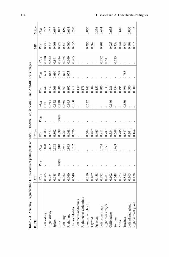
For the first Anatomy Benchmark, the following seven participants submitted algo-rithms, with their scores shown in Tables 7.3 and 7.4:

Dabbah et al. (P1A1) use a voxel-level trained solution based on classificationforests for landmark detection. Datasets are first aligned and downsampled to anisotropic resolution of 4mm per voxel. Features are the Hounsfield units at chosenrandom offsets from each landmark.

Gass et al. (P2A1) use multiatlas-based techniques for both segmentation andlandmark detection, focusing on modality- and anatomy-independent techniquesto be applied in a wide range of image modalities, in contrast to methods cus-tomized to a specific anatomy or modality. For segmentation, label propagationfrom several atlases to a target image is proposed. For landmark localization,consensus-based fusion of location estimates from several atlases identified by acustomized template-matching approach is used.

Huang et al. (P3A1) propose an automatic and robust coarse-to-fine liver imagesegmentation method. The workflow can be divided into four steps: liver local-ization, shape model fitting, appearance profile fitting and free-form deformation.

Jiménez del Toro et al. (P4A1) use a multiatlas-based segmentation approach.Multiple atlases identify the location of one or more structures in the patientvolume. The label volumes of the atlases are transformed using the image registra-tions of each atlas to the target volume. A stochastic gradient descent optimizationis performed for the desired metric during the process.

Kechichian et al. (P5A1) present an automatic multiple organ segmentationmethod based on a multilabel graph cuts using prior information of organ spa-tial relationships and shape. The former is derived from shortest-path pairwiseconstraints defined on a graph model of structure adjacency relations, and thelatter is represented by probabilistic organ atlases learned from a training dataset.

Spanier et al. (P6A1) describe a new generic method for the automatic rule-basedsegmentation of multiple organs from 3DCT scans. The rules determine the order


Table7.3

Anatomy1

segm

entatio

nDICEscores

ofparticipantson

Wb/CT,

ThA

b/CTce,W

b/MRT1andAb/MRT1cefsim

ages

DIC

ECT

CTce

MR

MRce

P2A1

P3A1

P7A1

P2A1

P3A1

P4A1

P5A1

P6A1

P7A1

P2A1

P2A1

Leftk

idney

0.805

-0.820

0.903

-0.921

0.747

0.631

0.820

0.730

0.782

Right

kidney

0.754

-0.802

0.877

-0.913

0.632

0.663

0.872

0.733

0.787

Spleen

0.688

-0.868

0.802

-0.852

0.768

0.690

0.891

0.668

0.689

Liver

0.830

0.892

0.910

0.899

0.892

0.918

0.806

0.747

0.914

0.822

0.847

Leftlung

0.952

-0.961

0.961

-0.955

0.853

0.848

0.965

0.533

0.650

Right

lung

0.960

-0.963

0.968

-0.965

0.892

0.975

0.969

0.900

0.664

Urinary

bladder

0.640

-0.732

0.676

-0.700

0.718

-0.805

0.656

0.280

Leftrectusabdominis

--

--

--

0.130

--

Right

rectus

abdominis

--

--

--

0.171

--

Lum

barvertebra

10.350

--

0.604

-0.522

0.447

--

0.396

0.060

Thyroid

0.469

--

0.469

--

0.004

--

0.367

Pancreas

0.438

--

0.465

--

0.155

--

0.356

Leftp

soas

major

0.772

-0.764

0.811

--

0.706

-0.792

0.801

0.644

Right

psoasmajor

0.787

-0.771

0.787

--

0.633

-0.811

Gallbladd

er0.102

--

0.334

-0.566

0.281

--

0.023

0.035

Sternum

0.648

-0.683

0.648

--

0.454

-0.713

0.358

Aorta

0.723

--

0.785

--

0.495

--

0.744

0.616

Trachea

0.822

--

0.847

-0.836

0.696

0.785

-0.736

Leftadrenalgland

0.165

--

0.204

--

0.000

--

0.109

0.000

Right

adrenalg

land

0.138

--

0.164

--

0.000

--

0.215

0.107


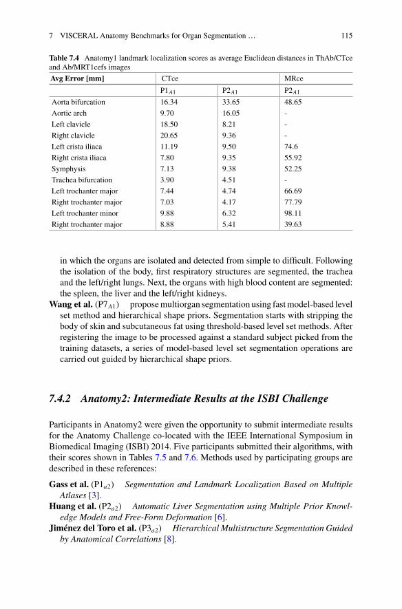
Table 7.4 Anatomy1 landmark localization scores as average Euclidean distances in ThAb/CTceand Ab/MRT1cefs images

Avg Error [mm] CTce MRce

P1A1 P2A1 P2A1Aorta bifurcation 16.34 33.65 48.65

Aortic arch 9.70 16.05 -

Left clavicle 18.50 8.21 -

Right clavicle 20.65 9.36 -

Left crista iliaca 11.19 9.50 74.6

Right crista iliaca 7.80 9.35 55.92

Symphysis 7.13 9.38 52.25

Trachea bifurcation 3.90 4.51 -

Left trochanter major 7.44 4.74 66.69

Right trochanter major 7.03 4.17 77.79

Left trochanter minor 9.88 6.32 98.11

Right trochanter major 8.88 5.41 39.63

in which the organs are isolated and detected from simple to difficult. Followingthe isolation of the body, first respiratory structures are segmented, the tracheaand the left/right lungs. Next, the organs with high blood content are segmented:the spleen, the liver and the left/right kidneys.

Wang et al. (P7A1) proposemultiorgan segmentation using fastmodel-based levelset method and hierarchical shape priors. Segmentation starts with stripping thebody of skin and subcutaneous fat using threshold-based level set methods. Afterregistering the image to be processed against a standard subject picked from thetraining datasets, a series of model-based level set segmentation operations arecarried out guided by hierarchical shape priors.

7.4.2 Anatomy2: Intermediate Results at the ISBI Challenge

Participants in Anatomy2 were given the opportunity to submit intermediate resultsfor the Anatomy Challenge co-located with the IEEE International Symposium inBiomedical Imaging (ISBI) 2014. Five participants submitted their algorithms, withtheir scores shown in Tables 7.5 and 7.6. Methods used by participating groups aredescribed in these references:

Gass et al. (P1a2) Segmentation and Landmark Localization Based on MultipleAtlases [3].

Huang et al. (P2a2) Automatic Liver Segmentation using Multiple Prior Knowl-edge Models and Free-Form Deformation [6].

Jiménez del Toro et al. (P3a2) Hierarchical Multistructure Segmentation Guidedby Anatomical Correlations [8].


Spanier et al. (P4a2) Rule-based ventral cavity multiorgan automatic segmenta-tion in CT scans [14].

Wang et al. (P5a2) Automatic multiorgan segmentation using fast model-basedlevel set method and hierarchical shape priors [16].

7.4.3 Anatomy2: Main Benchmark

Eight groups submitted algorithms for the final Anatomy2 Benchmark, with scoresreported in Tables 7.7 and 7.8. Approaches used are described in the followingreferences:

Gass et al. (P1A2) submitted amultiatlas-based segmentation and landmark local-isation method in images with large field of view [2].

Jiménez del Toro et al. (P2A2) submitted an algorithm based on hierarchicalmultiatlas-based segmentation for anatomical structures [7].

Kéchichian et al. (P3A2) submitted a generic multilabel graph cut method, whichuses location likelihood and spatial relationships between organs [12].

Li et al. (P4A2) submitted an automatic and robust coarse-to-fine liver image seg-mentation method [13].

Mai et al. (P5A2) submitted an approach for landmark detection in volumetricimages based on the popular Histograms of Oriented Gradients Descriptor (HOG)and linear support vector machines (SVM).

Spanier et al. (P6A2) submitted a rule-based algorithm [14, 15].Vincent et al. (P7A2) submitted a specific, automatic model-based framework for

segmenting the aorta, kidneys, liver, lungs and the psoas major muscles inWb/CTand ThAb/CTce images.

Wang et al. (P8A2) submitted the method described in [16].

7.4.4 Anatomy3

Five participants submitted algorithms to the Anatomy3 Benchmark before an initialkick-off deadline, with their scores reported in Table 7.9. Results from subsequentandmore recent submissions can be found in the online leaderboard.2 The approachessubmitted are described in the following references:

2http://visceral.eu:8080/register/Leaderboard.xhtml.

http://visceral.eu:8080/register/Leaderboard.xhtml


Table7.5

Anatomy2-ISB

Ichallengesegm

entatio

nDICEscores

forWb/CT,

ThA

b/CTce,W


ages

DIC

ECT

CTce

MR

MRce

P1a2

P2a2

P3a2

P5a2

P1a2

P2a2

P3a2

P4a2

P5a2

P1a2

P1a2

Leftk

idney

0.756

-0.678

0.729

0.885

-0.923

0.902

0.896

0.548

0.888

Right

kidney

0.679

-0.649

0.777

0.827

-0.905

-0.890

0.589

0.732

Spleen

0.684

-0.677

0.887

0.803

-0.859

0.934

0.842

0.646

0.785

Liver

0.798

0.911

0.823

0.904

0.882

0.922

0.908

-0.887

0.817

0.861

Leftlung

0.955

-0.969

0.971

0.960

-0.952

0.970

0.956

0.486

-

Right

lung

0.965

-0.967

0.972

0.966

-0.963

0.979

0.942

0.909

-

Urinary

bladder

0.636

-0.616

0.806

0.657

-0.680

-0.738

0.577

0.334

Leftrectusabdominis

--

--

--

--

--

-

Right

rectus

abdominis

--

--

--

--

--

-

Lum

barvertebra

10.333

-0.44

-0.548

-0.472

--

0.623

0.084

Thyroid

0.439

--

-0.315

--

-0.488

-

Pancreas

0.466

--

-0.442

--

--

-0.356

Leftp

soas

major

0.773

--

0.722

0.797

--

-0.737

0.765

0.654

Right

psoasmajor

0.78

--

0.764

--

--

0.752

--

Gallbladd

er0.078

-0.271

-0.212

-0.400

--

0.044

0.000

Sternum

0.63

--

0.712

0.612

--

-0.590

0.359

-

Aorta

0.724

--

-0.787

--

--

0.783

-

Trachea

0.837

-0.855

-0.839

-0.830

0.856

-0.747

-

Leftadrenalgland

0.282

--

-0.099

--

--

0.144

-

Right

adrenalg

land

0.133

--

-0.019

--

--

0.268

-


Table 7.6 Anatomy2-ISBI challenge landmark localization scores as average Euclidean distancesin Wb/CT, ThAb/CTce, Wb/MRT1 and Ab/MRT1cefs images

Avg Error [mm] CT CTce MR MRce

P1a2 P1a2 P1a2 P1a2Aorta bifurcation 19.05 36.22 252.49 61.28

Aortic arch 17.68 16.18 43.67 -

Left clavicle 9.27 16.26 13.05 -

Right clavicle 5.69 32.35 23.31 -

Left crista iliaca 7.7 13.93 23.29 88.92

Right crista iliaca 6.12 10.38 19.21 57.65

Symphysis 8.01 15.59 122.45 50.86

Trachea bifurcation 3.99 3.35 61.2 -

Left trochanter major 34.37 37.84 29.57 30.49

Right trochanter major 36.18 38.31 44.4 59.81

Left trochanter minor 5.16 11.22 18.51 28.54

Right trochanter major 4.06 12.64 62.4 34.84

Dicente Cid et al. (P1A3) participated with a fully automatic method for the seg-mentation of the lung volumes in CT [1].

He et al. (P2A3) submitted an automatic multiorgan segmentation based on multi-boost learning and statistical shape model search [4].

Heinrich et al. (P3A3) submitted a discrete medical image registration frameworkto multiorgan segmentation in different modalities [5].

Jiménez del Toro et al. (P4A3) contributed a hierarchical multiatlas multistructure segmentation approach guided by anatomical correlations (AnatSeg-Gspac) [9].

Kahl et al. (P5A3) proposed amethod for multiorgan segmentation in whole-bodyCT images based on a multiatlas approach [11].

7.4.5 Discussion

Participation in the various editions of the Anatomy Benchmarks allows us to answerquestions regarding popularity of tasks and imagemodalities, potentially also relatingto the (perceived) difficulty of each task/modality. Specifically, the popular modal-ity in Anatomy1 and Anatomy2 editions was contrast-enhanced CT, followed bystandard CT. Magnetic resonance imaging did not attract more than a single partic-ipant for the segmentation tasks, and only in the Anatomy2 landmark localizationtask, was able to attract two participants, potentially due to the relative difficultyof automatic analysis using this modality. Some algorithms were organ or modal-ity specific, so were only submitted for that anatomy, whereas other methods were


Table7.7

Anatomy2

Benchmarksegm

entatio

nDICEscores

forWb/CT,

ThA

b/CTce,W


ages

DIC

ECT

CTce

MR

MRce

P1A2

P2A2

P4A2

P7A2

P8A2

P1A2

P2A2

P3A2

P4A2

P6A2

P7A2

P8A2

P1A2

P1A2

Leftk

idney

0.778

0.784

-0.925

0.873

0.913

0.910

0.855

-0.829

0.943

0.927

0.808

0.845

Right

kidney

0.748

0.790

-0.866

0.871

0.914

0.889

0.805

-0.870

0.927

0.923

0.812

0.880

Spleen

0.671

0.703

--

0.914

0.781

0.721

0.812

-0.822

-0.867

0.684

0.659

Liver

0.831

0.866

0.831

0.934

0.934

0.908

0.882

0.925

0.937

-0.942

0.930

0.827

0.834

Leftlung

0.952

0.972

-0.970

0.960

0.961

0.959

0.955

-0.970

0.969

0.965

0.567

0.528

Right

lung

0.960

0.974

-0.970

0.962

0.965

0.962

0.953

-0.968

0.974

0.866

0.903

0.725

Urinary

bladder

0.666

0.698

--

0.713

0.683

0.674

0.774

--

--

0.709

0.205

Lrectus

abd

-0.551

--

--

0.444

0.111

--

--

--

Rrectus

abd

-0.498

--

--

0.453

0.211

--

--

--

L1

0.412

0.718

--

-0.624

0.523

0.486

--

--

0.415

0.077

Thyroid

0.450

0.549

--

-0.184

0.410

0.037

--

--

0.306

-

Pancreas

0.415

0.408

--

-0.460

0.406

0.544

--

--

0.196

0.372

Lpsoasmajor

0.777

0.806

-0.858

0.833

0.813

0.794

0.775

--

0.864

0.820

0.820

0.640

Rpsoasmajor

0.747

0.787

-0.848

0.828

-0.799

0.693

--

0.874

0.847

--

Gallbladd

er0.191

0.276

--

-0.381

0.484

--

--

-0.000

0.043

Sternum

0.633

0.742

--

-0.635

0.714

0.573

--

-0.773

0.006

-

Aorta

0.741

0.748

-0.823

0.660

0.785

0.758

0.535

--

0.838

-0.750

0.525

Trachea

0.840

0.888

--

-0.847

0.849

0.592

-0.851

--

0.731

-

Ladrgland

0.067

0.353

--

-0.250

0.331

0.000

--

--

0.151

0.048

Radrgland

0.186

0.355

--

-0.213

0.341

0.000

--

--

0.077

0.020


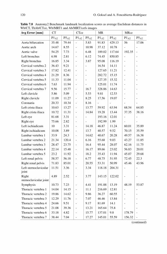
Table 7.8 Anatomy2 Benchmark landmark localization scores as average Euclidean distances inWb/CT, ThAb/CTce, Wb/MRT1 and Ab/MRT1cefs images


P1A2 P5A2 P1A2 P5A2 P1A2 P5A2 P1A2 P5A2Aorta bifurcation 35.48 79.44 - 5.83 91.83 429.13 56 17.06

Aortic arch 14.67 8.55 - 10.98 37.12 10.78 - -

Aortic valve 54.25 7.73 - 6.48 189.02 117.64 192.35 -

Left bronchus 6.98 2.81 - 6.12 74.45 850.85 - -

Right bronchus 16.85 3.34 - 3.87 95.08 116.19 - -

Cervical vertebra 2 36.43 9.21 - - 16.54 14.11 - -





Cervical vertebra 7 9.56 15.77 - 16.7 328.86 14.63 - -

Left clavicle 5.86 5.09 - 5.53 9.81 12.53 - -

Right clavicle 11.09 11.27 - 8.25 17.56 19.07 - -

Coronaria 20.33 10.34 - 8.16 - - - -

Left crista iliaca 10.63 13.27 - 13.77 59.92 63.94 68.54 64.85

Right crista iliaca 10.72 11.31 - 14.84 19.28 13.44 37.35 38.16

Left eye 81.68 3.31 - - 193.16 12.01 - -

Right eye 75.66 2.82 - - 192.99 1.99 - -

Left ischiadicum 10 3.31 - 14.18 46.87 11.24 60.01 35.89

Right ischiadicum 10.08 3.89 - 13.7 40.57 9.52 70.15 35.59

Lumbar vertebra 1 33.9 24.3 - 14.62 40.67 20.28 49.57 16.38

Lumbar vertebra 2 21.34 120.4 - 6.16 55.68 9.03 43.27 11.85

Lumbar vertebra 3 28.47 23.75 - 16.4 95.44 28.07 62.16 11.75

Lumbar vertebra 4 22.14 15.48 - 16.17 89.66 23.02 56.83 20.01

Lumbar vertebra 5 23.2 11.92 - 18.2 35.43 11.94 45.07 29.68

Left renal pelvis 58.57 56.18 - 6.77 48.75 51.95 72.45 22.3

Right renal pelvis 71.83 85.01 - 20.55 53.31 50.99 45.46 43.96

Left sternoclavicularjoint

11.51 3.36 - 3.34 118.18 204.31 - -

Rightsternoclavicular joint

4.89 2.52 - 3.77 143.15 122.02 - -

Symphysis 10.73 7.23 - 4.41 191.88 13.19 48.19 53.87

Thoracic vertebra 1 14.04 14.15 - 11.1 216.69 12.81 - -





Thoracic vertebra 6 33.18 4.82 - 15.77 137.01 9.8 178.79 -

Thoracic vertebra 7 38.44 7.04 - 17.27 145.01 55.59 156.32 -

(continued)


Table 7.8 (continued)


Thoracic vertebra 8 55.84 12.35 - 11.85 184.15 13.35 187.26 309.45





Trachea bifurcation 4.68 2.6 - 4.94 17 9.94 - -

Left trochantermajor

4.44 4.58 - 6.27 37.06 38.84 127.11 85.97

Right trochantermajor

4.77 6.19 - 3.7 64.89 97.45 68.21 71.75

Left trochanterminor

8.53 4.97 - 2.82 55.54 7.47 125.94 131.36

Right trochanterminor

6.57 4.49 - 2.67 157.91 9.13 30.6 41.91

Left tuberculum 8.45 120.91 - 12.68 17.5 53.16 - -

Right tuberculum 11.59 7.69 - 83.16 17.6 20.11 - -

Inferior vena cavabifurcation

16.14 10.19 - 14.14 88.35 239.12 80.31 19.99

Left ventricle 6.32 4.72 - - 129.68 803.14 - -

Right ventricle 7.14 5.28 - - 116.43 1076.85 - -

Xyphoid process 28.76 122.47 - 14.32 217.86 154.09 210.03 39.69

more general. Some participants with such generic methods seemingly pre-testedtheir methods on different inputs and only submitted them for the organs/modalitieswhere thesemethods could actually provide a value (i.e. satisfactory results), whereasother participants simply submitted their method for all organs/modalities, whetherthey generalized successfully or not.

Regarding the tasks, segmentation gathered a vast majority of the submissions.Most popular organs attempted in these benchmarkswere liver, lungs, spleen, kidneysandurinarybladder. Some structureswere segmentedbyvery fewmethods, e.g. rectusabdominis muscles.

In terms of segmentation results, the organs that obtained the highest DICE coef-ficient values for each modality were the lungs and the liver in CT and the kidneysand the liver in MRI. Other structures that achieved relatively accurate segmentationacross different Anatomy benchmarks include trachea, aorta, urinary bladder, psoasmajor muscles and spleen, with DICE coefficients ranging between 0.80 and 0.95.On the other hand, thyroid, adrenal glands, rectus abdominis muscles and gall blad-der have been shown to be the most difficult structures for segmentation, with DICEcoefficients below 0.5.

The landmark localization tasks have shown a large variation in performance evenfor the same method, but accurate results with average localization errors below 3


Table7.9

Anatomy3

Segm

entatio

nDIC

Ecoefficient

onCTvolumes

DIC

ECT

CTce

MRce

P1A3

P2A3

P4A3

P5A3

P1A3

P2A3

P4A3

P3A3

Leftk

idney

--

0.784

0.934

-0.91

0.91

0.862

Right

kidney

--

0.79

0.915

-0.922

0.889

0.855

Spleen

-0.874

0.703

0.87

-0.896

0.73

0.724

Liver

-0.923

0.866

0.921

-0.933

0.887

0.837

Leftlung

0.972

0.952

0.972

0.972

0.974

0.966

0.959

-

Right

lung

0.974

0.957

0.975

0.975

0.973

0.966

0.963

-

Urinary

bladder

--

0.698

0.763

--

0.679

0.494

Leftrectusabdominis

--

0.551

0.746

--

0.474

-

Right

rectus

abdominis

--

0.519

0.679

--

0.453

-

Lum

barvertebra

1-

-0.718

0.775

--

0.523

-

Thyroid

--

0.549

0.424

--

0.410

-

Pancreas

--

0.408

0.383

--

0.423

-

Leftp

soas

major

--

0.806

0.861

--

0.794

0.801

Right

psoasmajor

--

0.787

0.847

--

0.799

0.772

Gallbladd

er-

-0.276

0.19

--

0.484

-

Sternum

--

0.753

0.775

--

0.762

-

Aorta

--

0.761

0.847

--

0.721

-

Trachea

--

0.92

0.931

--

0.855

-

Leftadrenalgland

--

0.373

0.282

--

0.331

-

Right

adrenalg

land

--

0.355

0.22

--

0.342

-


voxels could be achieved, e.g. for the eyes and the trachea bifurcation. Modality alsohad a strong impact, with some structures being much easier to localize in CT (forinstance, sternoclavicular joints), whereas others in MRI (e.g. aorta bifurcation andthe coronaria).

Additional discussion and further information on the organization and the resultsof the Anatomy benchmarks can be found in [10].

7.5 Conclusion

During the VISCERALAnatomyBenchmarks, segmentation and landmark localiza-tion methods on large medical image datasets have been evaluated. Organization ofthese benchmarks led to the creation of large amounts of annotated medical imagingdata, which continue to be available beyond the end of the VISCERAL project (seeChap. 5). The use of a cloud-based evaluation not only represents an opportunityfor larger datasets, but also impacts the number of participants. However, the serieshas shown that yearly cycles of evaluation can attract larger numbers of participants,when sufficient data are provided for training and testing.

Acknowledgements The research leading to these results has received funding from the EuropeanUnion Seventh Framework Programme (FP7/2007-2013) under grant agreement 318068 (VIS-CERAL).

References

1. Dicente Cid Y, Jiménez del Toro OA, Depeursinge A, Müller H (2015) Efficient and fullyautomatic segmentation of the lungs in CT volumes. In: Goksel O, Jiménez del Toro OA,Foncubierta-Rodríguez A, Müller H (eds) CEUR workshop proceedings of the VISCERALanatomy3 organ segmentation challenge at ISBI, New York, USA

2. Gass T, Szekely G, Goksel O (2014) Multi-atlas segmentation and landmark localization inimages with large field of view. In: Menze B, Langs G, Montillo A, Kelm M, Müller H, ZhangS, CaiWT,Metaxas D (eds)MCV2014. LNCS, vol 8848. Springer, Cham, pp 171–180. doi:10.1007/978-3-319-13972-2_16

3. Goksel O, Gass T, Szekely G (2014) Segmentation and landmark localization based onmultipleatlases. In: Goksel O (ed) CEUR workshop proceedings of the VISCERAL challenge at ISBI.Beijing, China, pp 37–43

4. He B, Huang C, Jia F (2015) Fully automatic multi-organ segmentation based on multi-boostlearning and statistical shape model search. In: Goksel O, Jiménez del Toro OA, Foncubierta-Rodríguez A,Müller H (eds) CEURworkshop proceedings of the VISCERAL anatomy3 organsegmentation challenge at ISBI, New York, USA

5. Heinrich MP, Maier O, Handels H (2015) Multi-modal multi-atlas segmentation using discreteoptimisation and self-similarities. In: Goksel O, Jiménez del Toro OA, Foncubierta-RodríguezA, Müller H (eds) CEUR workshop proceedings of the VISCERAL anatomy3 organ segmen-tation challenge at ISBI, New York, USA

6. Huang C, Li X, Jia F (2014) Automatic liver segmentation using multiple prior knowledgemodels and free-form deformation. In: Goksel O (ed) CEUR workshop proceedings of theVISCERAL challenge at ISBI. Beijing, China, pp 22–24

http://dx.doi.org/10.1007/978-3-319-49644-3_5

http://dx.doi.org/10.1007/978-3-319-13972-2_16

http://dx.doi.org/10.1007/978-3-319-13972-2_16


7. Jiménez del Toro OA, Müller H (2014) Hierarchic multi–atlas based segmentation for anatom-ical structures: evaluation in the VISCERAL anatomy benchmarks. In: Menze B, Langs G,Montillo A, Kelm M, Müller H, Zhang S, Cai WT, Metaxas D (eds) MCV 2014. LNCS, vol8848. Springer, Cham, pp 189–200. doi:10.1007/978-3-319-13972-2_18

8. Jiménez del Toro OA, Müller H (2014) Hierarchical multi-structure segmentation guided byanatomical correlations. In: Goksel O (ed) CEUR workshop proceedings of the VISCERALchallenge at ISBI. Beijing, China, pp 32–36

9. Jiménez del Toro OA, Dicente Cid Y, Depeursinge A, Müller H (2015) Hierarchic anatomicalstructure segmentation guided by spatial correlations (anatseg-gspac): VISCERAL anatomy3.In: Goksel O, Jiménez del ToroOA, Foncubierta-RodríguezA,MüllerH (eds) CEURworkshopproceedings of the VISCERAL anatomy3 organ segmentation challenge at ISBI, New York,USA

10. Jiménez del Toro OA, Müller H, Krenn M, Gruenberg K, Taha AA, Winterstein M, Eggel I,FoncubiertaRodríguez A, Goksel O, Jakab A, Kontokotsios G, Langs G, Menze B, FernandezTS, Schaer R, Walley A, Weber M, Cid YD, Gass T, Heinrich M, Jia F, Kahl F, Kechichian R,Mai D, Spanier AB, Vincent G, Wang C, Wyeth D, Hanbury A (2016) Cloud-based evaluationof anatomical structure segmentation and landmark detection algorithms: VISCERAL anatomybenchmarks. IEEE Trans Med Imaging 35(11):2459–2475

11. Kahl F, Alvén J, Enqvist O, Fejne F, Ulén J, Fredriksson J, LandgrenM, LarssonV (2015) Goodfeatures for reliable registration in multi-atlas segmentation. In: Goksel O, Jiménez del ToroOA,Foncubierta-RodríguezA,MüllerH (eds)CEURworkshopproceedings of theVISCERALanatomy3 organ segmentation challenge at ISBI, New York, USA

12. Kéchichian R,Valette S, SdikaM,DesvignesM (2014) Automatic 3Dmultiorgan segmentationvia clustering and graph cut using spatial relations and hierarchically-registered atlases. In:Menze B, Langs G, Montillo A, Kelm M, Müller H, Zhang S, Cai WT, Metaxas D (eds) MCV2014. LNCS, vol 8848. Springer, Cham, pp 201–209. doi:10.1007/978-3-319-13972-2_19

13. Li X, Huang C, Jia F, Li Z, Fang C, Fan Y (2014) Automatic liver segmentation using statisticalprior models and free-form deformation. In: Menze B, Langs G, Montillo A, Kelm M, MüllerH, Zhang S, Cai WT, Metaxas D (eds) MCV 2014. LNCS, vol 8848. Springer, Cham, pp181–188. doi:10.1007/978-3-319-13972-2_17

14. SpanierAB, Joskowicz L (2014)Rule-based ventral cavitymulti-organ automatic segmentationin CT scans. In: Goksel O (ed) CEUR workshop proceedings of the VISCERAL challenge atISBI. Beijing, China, pp 16–21

15. SpanierAB, Joskowicz L (2014)Rule-based ventral cavitymulti-organ automatic segmentationin CT scans. In:Menze B, Langs G,Montillo A, KelmM,Müller H, Zhang S, CaiWT,MetaxasD (eds) MCV 2014. LNCS, vol 8848. Springer, Cham, pp 163–170. doi:10.1007/978-3-319-13972-2_15

16. Wang C, Smedby O (2014) Automatic multi-organ segmentation using fast model based levelset method and hierarchical shape priors. In: Goksel O (ed) CEUR workshop proceedings ofthe VISCERAL challenge at ISBI. Beijing, China, pp 25–31

http://dx.doi.org/10.1007/978-3-319-13972-2_18

http://dx.doi.org/10.1007/978-3-319-13972-2_19

http://dx.doi.org/10.1007/978-3-319-13972-2_17

http://dx.doi.org/10.1007/978-3-319-13972-2_15

http://dx.doi.org/10.1007/978-3-319-13972-2_15


Open Access This chapter is licensed under the terms of the Creative Commons Attribution- Non-

Commercial 2.5 International License (http://creativecommons.org/licenses/by-nc/2.5/), which

permits any noncommercial use, sharing, adaptation, distribution and reproduction in any medium

or format, as long as you give appropriate credit to the original author(s) and the source, provide a

link to the Creative Commons license and indicate if changes were made.

The images or other third party material in this chapter are included in the chapter’s Creative

Commons license, unless indicated otherwise in a credit line to the material. If material is not

included in the chapter’s Creative Commons license and your intended use is not permitted by

statutory regulation or exceeds the permitted use, you will need to obtain permission directly from

the copyright holder.

http://creativecommons.org/licenses/by-nc/2.5/

Chapter 7 VISCERAL Anatomy Benchmarks for Organ ...7 VISCERAL Anatomy Benchmarks for Organ...

Documents

Transcript of Chapter 7 VISCERAL Anatomy Benchmarks for Organ ...7 VISCERAL Anatomy Benchmarks for Organ...