Chapter 7 Symmetric circulation models - MIT OpenCourseWare · Symmetric circulation models 111...

Chapter 7

Symmetric circulation models

Supplemental reading

Lorenz (1967)

Held and Hou (1980)

Schneider and Lindzen (1977)

Schneider (1977)

Lindzen and Hou (1988)

Walker and Schneider (2004)

As we noticed in our perusal of the data atmospheric fields are far from being zonally symmetric Some of the deviation from symmetry is forced by the inhomogeneity of the earthrsquos surface and some is autonomous (travshyelling cyclones for example) The two are related for example the storm paths along which travelling cyclones travel are significantly determined by the planetary scale waves forced by inhomogeneities in the earthrsquos surface Nevertheless the zonally averaged circulation has over the centuries been the object of special attention Indeed the term lsquogeneral circulationrsquo is freshyquently taken to mean the zonally averaged behavior This is the viewpoint of Lorenz (1967)

You are urged to read chapters 13 and 4 of Lorenz Chapter 1 is a short and especially insightful discussion of the methodology of studying the atmosphere As is generally the case in this field there will be views in

109

110 Dynamics in Atmospheric Physics

Lorenz which are not universally agreed on but this hardly diminishes its value

There are several reasons for focussing on the zonally averaged circulashytion

1 Significant motion systems like the tropical tradewinds are well deshyscribed by zonal averages

2 The circulation of the atmosphere is only a small perturbation on a rigidly rotating basic state which is zonally symmetric

3 The zonally averaged circulation is a convenient subset of the total circulation

Our approach in this chapter will be to inquire how the atmosphere would behave in the absence of eddies It is hoped that a comparison of such results with observations will lend some insight into what maintains the observed zonally averaged state In particular discrepancies may point to the role of eddies in maintaining the zonal average This has been a matter of active controversy to the present

71 Historical review

A very complete historical treatment of this subject is given in chapter 4 of Lorenz We will only present a limited sketch here The first treatment of contemporary relevance was that of Hadley (1735) Hadleyrsquos aim was to explain the easterly (actually northeasterly in the Northern Hemisphere) tradewinds of the tropics and the prevailing westerlies of middle latitudes His brief explanation is summarized in Figure 71 Ignoring Hadleyrsquos error in assuming conservation of velocity rather than angular momentum Hadleyrsquos argument ran roughly as follows

1 Warm air rises at the equator and flows poleward at upper levels apshyproximately conserving angular momentum (In view of the remarks at the end of Chapter 6 it is not however at all obvious why one would have a meridional circulaton at all We will discuss this later) Beshycause the distance from the axis of rotation diminishes with increasing latitude large westerly currents are produced at high latitudes

111 Symmetric circulation models

Figure 71 A schematic representation of the general circulation of the atmosphere as envisioned by Hadley (1735)

2 The westerly currents would be far larger than observed It is therefore presumed that friction would reduce westerly currents As a result the return flow at the surface will have a momentum deficit leading to tropical easterlies

(In what sense does Hadleyrsquos argument constitute an lsquoexplanationrsquo) The above model was generally accepted for over a century The main

criticism of this model was that it predicted northwesterly winds at midlatshyitudes whereas nineteenth century data suggested southwesterly winds (in the Northern Hemisphere) This difficulty was answered independently by Ferrel (1856) and Thomson (1857) Their hypothesized solution is shown in Figure 72 Briefly Ferrel and Thomson supplemented Hadleyrsquos


Figure 72 The general circulation of the atmosphere according to Thomson (1857)

arguments as follows They noted that at the latitude at which zonal flow is zero there must be a maximum in pressure (Why) and that within the frictional layer next to the surface a shallow flow will be established down pressure gradients leading to the reversed cell shown in Figure 72 (today referred to as a Ferrel cell) By allowing the Hadley circulation to remain at upper levels the tropics can continue to supply midlatitudes with angular momentum which presumably is communicated to the Ferrel cell by friction

Although there was a general acceptance of the Ferrel-Thomson model of the general circulation in the late nineteenth century there was also a general uneasiness due to the obvious fact that the observed circulation was not zonally symmetric Moreover all the models we have discussed were developed in only a qualitative verbal way This is of course not surprising since the quantitative knowledge of atmospheric heating turbulent transfer


and so forth was almost completely lacking So was virtually any information about the atmosphere above the surface ndash except insofar as cloud motions indicated upper level winds

In 1926 Jeffreys put forth an interesting and influential criticism of all symmetric models as an explanation of midlatitude surface westerlies He began with an equation for zonal momentum (viz Equation 618)

partu partu partu partu uv tan φ uw partt

+ upartx

+ vparty

+ wpartz

minus a

+ a

1 partp 1 = minus

ρ partx + 2Ωv sinφ + 2Ωw cos φ +

ρ( middot τ )x (71)

For the purposes of Jeffreysrsquo argument (71) can be substantially simplified Steadiness and zonal symmetry (no eddies) imply part = part = 0 Scaling shows

partt partx

that

uw uv tan φ 2Ωw cos φ 2Ωv sinφ

a a

(What about the equator) In addition

partu uv tan φ v partu uv tanφ v part vparty

minus a

= a partφ

minus a

= a cosφ partφ

(u cosφ)

Thus (71) becomes

v part partu 1

a cosφ partφ(u cosφ) + w

partz minus 2Ωv sinφ =


Jeffreys further set

part partu ( τ )x = micro (73) middot

partz partz

Integrating (72) over all heights yields

infin ρv part infin partu (u cosφ) dz + ρw dz

0 a cos φ partφ 0 partz


infin partu minusCD u 2 0 (74)minus2Ω sin φ ρ0v dz = minusmicro =partz0 0

2where CD is the surface drag coefficient and CD u0 is the usual phenomenoshylogical expression for the surface drag Note that the earthrsquos angular momenshytum cannot supply momentum removed by surface drag (since there is no net meridional mass flow ie

0infin ρ0v dz = 0) Thus CD u

20 must be balanced

by the advection of relative momentum Jeffreys argued that the integrals on the left-hand side of (74) would be dominated by the first integral evaluated within the first kilometer or so of the atmosphere Underlying his argument was the obvious lack of data to do otherwise He then showed that this inshytegral was about a factor of 20 smaller than CD u0

2 He concluded that the maintenance of the surface westerlies had to be achieved by the neglected eddies It may seem odd that Jeffreys who so carefully considered the effect of the return v-flow on the Coriolis torque ignored it for the transport of relative momentum However since it was the Ferrel cell he was thinking of its inclusion would not have altered his conclusion What he failed to note was that in both Hadleyrsquos model and that of Ferrel and Thomson it was the Hadley cell which supplied westerly momentum to middle latitudes Thus Jeffreysrsquo argument is totally inconclusive it certainly is not a proof that a symmetric circulation would be impossible (though this was sometimes claimed in the literature)

A more balanced view was presented by Villem Bjerknes (1937) towards the end of his career Bjerknes suggested that in the absence of eddies the atmosphere would have a Ferrel-Thomson circulation ndash but that such an atshymosphere would prove unstable to eddies This suggestion did not however offer any estimate of the extent to which the symmetric circulation could explain the general circulation and the extent to which eddies are essential

Ed Schneider and I attempted to answer this question by means of a rather cumbersome numerical calculation (Schneider and Lindzen 1977 Schneider 1977) The results shown in Figure 73 largely confirm Bjerknesrsquo suggestion The main shortcoming of this calculation was that it yielded a zonal jet that was much too strong Surface winds were also a little weaker than observed but on the whole the symmetric circulation suffered from none of the inabilities Jeffreys had attributed to it In order to see how the symmetric circulation works it is fortunate that Schneider (1977) discovered a rather simple approximate approach to calculating the Hadley circulation Held and Hou (1980) explored this approximation in some detail We shall


briefly go over the Held and Hou calculations



Figure 73 Example of an eddy-free symmetric circulation found by Schneider (1977) Panel (a) shows contours of zonal wind (contour intervals of 15msminus1) Panel (b) shows streamfunction contours (contour intervals of 1012 gsminus1) Panel (c) shows temperature contours (contour intervals of 10 K)


72 Held and Hou calculations

Held and Hou restrict themselves to a Boussinesq fluid of depth H For such a fluid the continuity equation is simplified to

middot u = 0 (75)

With (75) as well as the assumptions of steadiness and zonal symmetry and the retention of only vertical diffusion in the viscous stress and thermal conduction terms our remaining equations of motion become

uv tan φ part partu (uu)minus f = ν (76) middot

v minus

a partz partz 2Ω sinφ

u2 tan φ 1 partΦ part

partv

middot (uv) + fu + a

= minusa partφ

+ partz

νpartz

(77)

(uΘ) = part

νpartΘ (Θ minus ΘE)

(78) middot partz partz

minus τ

and partΦ Θ

= g (79) partz Θ0

(NB Φ = pρ) The quantity ΘE is presumed to be a lsquoradiativersquo equilibrium

temperature distribution for which we adopt the simplified form

ΘE(φ z)

1 2

H

+ P2(sinφ) + ΔV z minus (710) equiv 1 minusΔHΘ0 3 3 2

where P2(x) equiv 1 2 H(3x minus1) x = sinφ Θ0 = ΘE(0 ) ΔH = fractional potenshy2 2

tial temperature drop from the equator to the pole ΔV = fractional potential temperature drop from H to the ground and τ is a lsquoradiativersquo relaxation time (The reader should work out the derivation of Equations 76ndash79 NB In the Boussinesq approximation density is taken as constant except where it is multiplied by g The resulting simplifications can also be obtained for a fully stratified atmosphere by using the log-pressure coordinates described in Chapter 4)


The boundary conditions employed by Held and Hou are

no heat conduction

partu partv partΘ = = = w = 0 at z = H (711)

partz partz partz rigid top

no stress

partΘ = w = 0 at z = 0 (712)

partz

partu partv ν = Cu ν = Cv at z = 0 (713) partz partz

linearization of surface stress conditions

v = 0 at φ = 0 (714)

symmetry about the equator

The quantity C is taken to be a constant drag coefficient Note that this is not the same drag coefficient that appeared in (74) neither is the expression for surface drag which appears in (713) the same As noted in (713) the expression is a linearization of the full expression The idea is that the full expression is quadratic in the total surface velocity ndash of which the contribution of the Hadley circulation is only a part The coefficient C results from the product of CD and the lsquoambientrsquo surface wind

When ν equiv 0 we have already noted that our equations have an exact solution

v = w = 0 (715)

Θ = ΘE (716)

and

u = uE (717)

where uE satisfies


part

uE 2 tan φ

g partΘE

partz fuE +

a = minus

aΘ0 partφ (where y = aφ) (718)

If we set uE = 0 at z = 0 the appropriate integral of (718) is (see Holton 1992 p 67)

12

uE z = 1 + 2R minus 1 cos φ (719)

Ωa H

where

gHΔHR = (720)

(Ωa)2

When R 1

uE z = R cosφ (721)

Ωa H Why isnrsquot the above solution at least approximately appropriate Why

do we need a meridional solution at all Hadley already implicitly recognized that the answer lies in the presence of viscosity A theorem (referred to as lsquoHidersquos theoremrsquo) shows that if we have viscosity (no matter how small) (715)ndash(719) cannot be a steady solution of the symmetric equations

721 Hidersquos theorem and its application

The proof of the theorem is quite simple We can write the total angular momentum per unit mass as

M equiv Ωa 2 cos 2 φ + ua cosφ (722)

(recall that ρ is taken to be lsquoconstantrsquo) and (76) may be rewritten

part2M middot (uM) = ν partz2

(723)


Now suppose that M has a local maximum somewhere in the fluid We may then find a closed contour surrounding this point where M is constant If we integrate (723) about this contour the contribution of the left-hand side will go to zero (Why) while the contribution of the right-hand side will be negative (due to down gradient viscous fluxes) Since such a situation is inconsistent M cannot have a maximum in the interior of the fluid We next consider the possibility that M has a maximum at the surface We may now draw a constant M contour above the surface and close the contour along the surface (where w = un = 0) Again the contribution from the left-hand side will be zero The contribution from the right-hand side will depend on the sign of the surface wind If the surface wind is westerly then the contribution of the right-hand side will again be negative and M therefore cannot have a maximum at the surface where there are surface westerlies If the surface winds are easterly then there is indeed a possibility that the contribution from the right-hand side will be zero Thus the maximum value of M must occur at the surface in a region of surface easterlies1 An upper bound for M is given by its value at the equator when u = 0 that is

Mmax lt Ωa 2 (724)

Now uE as given by (719) implies (among other things) westerlies at the equator and increasing M with height at the equator ndash all of which is forshybidden by Hidersquos theorem ndash at least for symmetric circulations A meridional circulation is needed in order to produce adherence to Hidersquos theorem

Before proceeding to a description of this circulation we should recall that in our discussion of observations we did indeed find zonally averaged westerlies above the equator (in connection with the quasi-biennial oscillashytion for example) This implies the existence of eddies which are transporting angular momentum up the gradient of mean angular momentum

A clue to how much of a Hadley circulation is needed can be obtained by seeing where uE = uM by uM we mean the value of u associated with M = Ωa2 (viz Equation 724) From (722) we get

Ωa sin2 φ uM = (725)

cos φ

1It is left to the reader to show that M cannot have a maximum at a stress-free upper surface


Setting uE = uM gives an equation for φ = φlowast For φ lt φlowast uE violates Hidersquos theorem

sin2 φlowast [(1 + 2R)12 minus 1] cos φlowast = (726)

cosφlowast

(Recall that R equiv gHΔH ) (Ωa)2

Solving (726) we get

φlowast = tanminus1[(1 + 2R)12 minus 1]12 (727)

For small R

φlowast = R12 (728)

Using reasonable atmospheric values

g = 98 msminus2

H = 15 104 m

Ω = 2π(864 104 s)

a = 64 106 m

and

ΔH sim 13

we obtain from (720)

R asymp 226

and

R12 asymp 48


and from (728)

φlowast asymp 30

Thus we expect a Hadley cell over at least half the globe2

722 Simplified calculations

Solving for the Hadley circulation is not simple even for the highly simplified model of Held and Hou However Schneider and Held and Hou discovered that the solutions they ended up with when viscosity was low were approxishymately constrained by a few principles which served to determine the main features of the Hadley circulation

1 The upper poleward branch conserves angular momentum

2 The zonal flow is balanced and

3 Surface winds are small compared to upper level winds

In addition

4 Thermal diffusion is not of dominant importance in Equation 78

Held and Hou examine in detail the degree to which these principles are valid and you are urged to read their work However here we shall merely examine the implications of items (1)ndash(4) and see how these compare with the numerical solutions from Held and Hou Principle (1) implies

Ωa sin2 φ u(H φ) = uM = (729)

cos φ 2The choice ΔH = 13 is taken from Held and Hou (1980) and corresponds to ΘE

varying by about 100 between the equator and the poles This indeed is reasonable for radiative equilibrium However more realistically the atmosphere is at any moment more nearly in equilibrium with the sea surface (because adjustment times for the sea are much longer than for the atmosphere) and therefore a choice of ΔH asymp 16 may be more appropriate This leads to R12 asymp 34 and φlowast asymp 20 which is not too different from what was obtained for ΔH = 13 This relative insensitivity of the Hadley cell extent makes it a fairly poor variable for distinguishing between various parameter choices


Principle (2) implies

u2 tan φ 1 partΦ fu + = (730)

a minusa partφ

Evaluating (730) at z = H and z = 0 and subtracting the results yields

tan φ f [u(H) minus u(0)] + [u 2(H) minus u 2(0)]

a 1 part

= minusa partφ

[Φ(H) minus Φ(0)] (731)

Integrating (79) from z = 0 to z = H yields

macrΦ(H) minus Φ(0) =

g Θ (732)

H Θ0

where Θ is the vertically averaged potential temperature Substituting (732) into (731) yields a simplified lsquothermal windrsquo relation

f [u(H) minus u(0)] + tan φ

[u 2(H) minus u 2(0)] = gH partΘ

(733) a

minusaΘ0 partφ

Principle (3) allows us to set u(0) = 0 Using this and (729) (733) becomes

Ωa sin2 φ tan φ Ω2a2 sin4 φ gH partΘ2Ω sin φ + = (734)

cosφ a cos2 φ minusaΘ0 partφ

Equation 734 can be integrated with respect to φ to obtain

macr macr Ω2 2Θ(0) minus Θ(φ)=

a sin4 φ (735)

Θ0 gH 2 cos2 φ

Note that conservation of angular momentum and the maintenance of a balshyanced zonal wind completely determine the variation of Θ within the Hadley regime Moreover the decrease of Θ with latitude is much slower near the equator than would be implied by ΘE

Finally we can determine both Θ(0) and the extent of the Hadley cell φH with the following considerations


1 At φH temperature should be continuous so

macr = ΘE(φH) (736) Θ(φH)

2 From Equation 78 we see that the Hadley circulation does not produce net heating over the extent of the cell For the diabatic heating law in Equation 78 we therefore have

φH φH

macr macrΘ cosφdφ = ΘE cosφdφ (737) 0 0

Substituting (735) into (736) and (737) yields the two equations we need in order to solve for φH and Θ(0) The solution is equivalent to matching (735) to ΘE so that lsquoequal areasrsquo of heating and cooling are produced This is schematically illustrated in Figure 74 Also shown are uM (φ) and uE(φ)

The algebra is greatly simplified by assuming small φ Then (735) becomes

Θ Θ(0) macr 1 Ω2a2

Θ0 asymp

Θ0 minus

2 gH φ4 (738)

and (710) becomes

macr macrΘE ΘE(0) = minus ΔHφ

2 (739) Θ0 Θ0

Substituting (738) and (739) into (736) and (737) yields

Θ(0) ΘE(0) 5

Θ0 =

Θ0 minus

18 RΔH (740)

and

12

φH = R (741) 3

5


Figure 74 Schematic drawings of the vertical mean potential temperature distribution (upper figure) and the zonal wind distribution at the top of the atmosphere (lower figure) With Newtonian cooling (linear in Θ) conservation of potential temperature requires that the shaded areas be equal Note that this idealized circulation increases the baroclinicity of the flow between φlowast (where uE = UM ) and φH


(Remember that gHΔH for a slowly rotating planet such as Venus φH2R equivΩ2a

can extend to the pole)

We see that continuity of potential temperature and conservation of angular momentum and potential temperature serve to determine the meridshyional distribution of temperature the intensity of the Hadley circulation will be such as to produce this temperature distribution In section 102 of Houghton 1977 there is a description of Charneyrsquos viscosity dominated model for a meridional circulation In that model Θ = ΘE and u = uE except in thin boundary layers and the meridional velocity is determined by

urequiring that fv balance the viscous diffusion of momentum ν partpartz

2

2 Such a model clearly violates Hidersquos theorem A more realistic viscous model is deshyscribed by Schneider and Lindzen (1977) and Held and Hou (1980) wherein the meridional circulation is allowed to modify Θ through the following linshyearization of the thermodynamic energy equation

partΘ minusw = (Θ minus ΘE)τ partz

where partpartz Θ is a specified constant In such models the meridional circulation

continues with gradual diminution to high latitudes rather than ending abruptly at some subtropical latitude ndash as happens in the present lsquoalmost inviscidrsquo model On the other hand the modification of Θ (for the linear viscous model) is restricted to a neighborhood of the equator given by

φ sim Rlowast14

where

τν

gH

Rlowast equiv 4H Ω2a2

ΔV

When Rlowast14 ge R12 (viz Equation 728) then a viscous solution can be comshypatible with Hidersquos theorem Note however that linear models cannot have surface winds (Why Hint consider the discussion of Jeffreysrsquo argument)

Returning to our present model there is still more information which can be extracted Obtaining the vertically integrated flux of potential temshy


perature is straightforward

1 H 1 part

(vΘcosφ) dz =ΘE minus Θ

(742) H 0 a cosφ partφ τ

In the small φ limit ΘE and Θ are given by (738)ndash(741) and (742) can be integrated to give

1 H

vΘ dz Θ0 0

5

512 HaΔH

⎡ φ

φ 3

φ 5⎤

=18 3 τ

R32 ⎣ φH

minus 2 φH

+ φH

⎦ (743)

Held and Hou are also able to estimate surface winds on the basis of this simple model For this purpose additional assumptions are needed

1 One must assume either (a) the meridional flow is primarily confined to thin boundary layers adjacent to the two horizontal boundaries or that (b) profiles of u and Θ are self-similar so that

u(z) minus u(0) Θ(z) minusΘ(0)

u(H) minus u(0)asymp

Θ(H) minus Θ(0)

(We shall employ (a) because itrsquos simpler)

2 Neither the meridional circulation nor diffusion affects the static stashybility so that

Θ(H) minus Θ(0) asymp ΔV

Θ0

(This requires that the circulation time and the diffusion time both be longer than τ a serious discussion of this would require consideration of cumulus convection)

With assumptions (1) and (2) above we can write


1 H

vΘ dz asymp V ΔV (744) Θ0 0

where V is a mass flux in the boundary layers With (744) (743) allows us to solve for V

Similarly we have for the momentum flux

H

vu dz asymp V uM (745) 0

To obtain the surface wind we vertically integrate (723) (using (722) and (713)) to get

1 part H

cos 2 φ uv dz = minusCu(0) (746) a cos2 φ partφ 0

From (743)ndash(746) we then get

⎡ 2 4 6⎤

25 ΩaHΔH R2 φ 10 φ 7 φ

Cu(0) asymp minus 18 τ ΔV

⎣ φH

minus 3 φH

+3 φH

⎦ (747)

Equation 747 predicts surface easterlies for

312

φ lt φH (748) 7

and westerlies for

312

φH lt φ lt φH (749) 7

For the parameters given following Equation 728 the positions of the upper level jet and the easterlies and westerlies are moderately close to those observed It can also be shown that for small ν the above scheme leads to a Ferrel cell above the surface westerlies We will return to this later For the moment we wish to compare the results of the present simple analysis with the results of numerical integrations of Equations 75ndash714


723 Comparison of simple and numerical results

Unfortunately the results in Held and Hou are for H = 8 103m rather timesthan 15times104m From our simple relations we correctly expect this to cause features to be compressed towards the equator Also Held and Hou adopted the following values for τ C and ΔV

τ = 20 days

C = 0005 msminus1

ΔV = 18

Figure 75 Zonal wind at z = H for three values of ν compared with the simple model for the limit ν 0 (from Held and Hou 1980 rarr

Figures 75ndash78 compare zonal winds at z = H M at z = H heat flux and surface winds for our simple calculations and for numerical integrations with various choices of ν In general we should note the following

1 As we decrease ν the numerical results more or less approach the simple results and for ν = 5m2sminus1 (generally accepted as a lsquosmallrsquo value) our simple results are a decent approximation (In fact however reducing ν much more does not convincingly show that the limit actually is reached since the numerical solutions become unsteady)


Figure 76 A measure of M namely ((Ωa2 minusM)a) evaluated at z = H as a function of φ for diminishing values of viscosity ν Note that zero corresponds to conservation of M (from Held and Hou 1980)

Figure 77 Meridional heat fluxes for various values of ν ndash as well as the theoretical limit based on the simple calculations (from Held and Hou 1980)


Figure 78 Surface wind for various values of ν and the theoretical inviscid limit based on simple calculations (from Held and Hou 1980)

2 The presence of modest vertical viscosity increass and broadens both heat flux and the distribution of surface winds (Why) Viscosity also reduces the magnitude of broadens and moves poleward the upper level jet

3 Very near the equator the numerical results do not quite converge to constant M at z = H The reason for this can be seen in Figures 79 and 710 where meridional cross sections are shown for the meridional stream functions and zonal wind

Note that the upward branch of the Hadley cell does not rise solely at the equator (as supposed in the simple theory) but over a 10 minus minus15

neighbourhood of the equator Note also the emergence of the Ferrel cell at small ν

73 Summary and difficulties

Before summarizing what all this tells us about the general circulation let us return to Figure 73 We see that Schneiderrsquos symmetric circulation which is by and large consistent with Held and Hoursquos also manages to predict an elevated tropical tropopause height and the associated tropopause lsquobreakrsquo at


Figure 79 Meridional streamfunctions and zonal winds In the left part of the figure the streamfunction ψ is given for ν = 25 10 and 5 m2sminus1 with a contour interval of 01 ψmax The value of 01 ψmax (m

2sminus1) is marked by a pointer The right part of each panel is the corresponding zonal wind field with contour intervals of 5 msminus1 The shaded area indicates the region of easterlies (from Held and Hou 1980)


Figure 710 Same as Figure 79 but for ν = 25 10 and 05 m2sminus1 Note the emergence of a Ferrel cell in the ψ-field where ψ lt 0 (indicated by shading) (from Held and Hou 1980)


the edge of the Hadley circulation The midlatitude tropopause somewhat artificially reflects the assumed ΘE distribution The elevated tropopause in the tropics results from the inclusion of cumulus heating

731 Remarks on cumulus convection

Cumulus heating will not be dealt with in these lectures but for the moment three properties of cumulus convection should be noted

1 It is in practice the primary mechanism for carrying heat from the surface in the tropics

2 Cumulus towers for simple thermodynamic reasons extend as high as 16 km and appear to be the determinant of the tropical tropopause height and the level of Hadley outflow Remember that tropical cirshyculations tend to wipe out horizontal gradients Thus the tropopause tends to be associated with the height of the deepest clouds

3 Cumulus convection actively maintains a dry static stability (as reshyquired in the calculation of Hadley transport) This is explained in Sarachik (1985)

A more detailed description of cumulus convection (and its parameterization) can be found in Emanuel (1994)as well as in Lindzen (1988b)

732 Preliminary summary

On the basis of our study of symmetric circulations (so far) we find the following

1 Symmetric solutions yield an upper level jet in about the right place but with much too large a magnitude

2 Symmetric circulations yield surface winds of the right sign in about the right place In the absence of vertical diffusion magnitudes are too small but modest amounts of vertical diffusion corrects matters and cumulus clouds might provide this lsquodiffusionrsquo (Schneider and Lindzen 1976 discuss cumulus friction)


3 Calculated Hadley circulations have only a finite extent In contrast to Hadleyrsquos and Ferrel and Thomsonrsquos diagnostic models the upper branch does not extend to the poles Thus our Hadley circulation canshynot carry heat between the tropics and the poles and cannot produce the observed polendashequator temperature difference

4 The calculated temperature distribution does not have the pronounced equatorial minimum at tropopause levels that is observed (viz Figshyure 511)

5 Although not remarked upon in detail the intensity of the Hadley circulation shown in Figure 710 is weaker than what is observed

At this point we could glibly undertake to search for the resolution of the above discrepancies in the role of the thus far neglected eddies However before doing this it is important to ask whether our symmetric models have not perhaps been inadequate in some other way besides the neglect of eddies

74 Asymmetry about the equator

Although we do not have the time to pursue this (and most other matters) adequately the reader should be aware that critical reassessments are essenshytial to the scientific enterprise ndash and frequently the source of truly important problems and results What is wrong with our results is commonly more important than what is right A particular shortcoming will be discussed here namely the assumption that annual average results can be explained with a model that is symmetric about the equator The importance of this shortcoming has only recently been recognized (This section is largely based on the material in a paper by Lindzen and Hou 1988) This fact alone should encourage the reader to adopt a more careful and critical attitude

What is at issue in the symmetry assumption can most easily be seen by looking at some data for the meridional circulation itself Thus far we have not paid too much attention to this field Figure 711 shows the meridional circulation for solstitial conditions Not surprisingly it is not symmetric about the equator More surprising however is the degree of asymmetry the lsquowinterrsquo cell extends from well into the summer hemisphere (sim 20) to well into the winter hemisphere (sim 30) whereas the lsquosummerrsquo cell barely


Figure 711 Time average meridional-height cross sections of the streamfunction for the mean meridional circulation Units 1013 gsminus1 contour intervals 02 1013 gsminus1 timesDecemberndashFebruary 1963ndash73 (upper panel) and JunendashAugust 1963ndash73 (lower panel) (from Oort 1983)


exists at all Figures 510 and 511 show meridional sections of zonally avshyeraged zonal wind and temperature for solstitial conditions Within about 20ndash25 of the equator these fields are symmetric about the equator Thus in this region at least an average over winter and summer of these fields will still give the solstitial distributions Finally Figure 712 shows the monthly means of the meridional circulation for each of the twelve months of the year This figure is a little hard to interpret since it extends to only 15S However to a significant extent it suggests that except for the month of April the asymmetric solstitial pattern is more nearly characteristic of every month than is the idealized symmetric pattern invoked since Hadley in the eighteenth century Clearly the assumption of such symmetry is suspect

Some insight into what is going on can interestingly enough be gotshyten from the simple lsquoequal arearsquo argument This is shown in Lindzen and Hou (1988) We will briefly sketch their results here They studied the axishyally symmetric response to heating centered off the equator at some latitude φ0 Thus Equation 710 was replaced by

ΘE ΔH z 1

Θ0

sim3 H

minus2

(750) = 1 + (1 minus 3(sin φ minus sinφ0)2) + ΔV

The fact that φ0 = 0 substantially complicates the problem Now the northshyward and southward extending cells will be different Although we still reshyquire continuity of temperature at the edge of each cell the northward extent of the Hadley circulation φH+ will no longer have the same magnitude as the southward extent minusφHminus Moreover the lsquoequal arearsquo argument must now be applied separately to the northern and southern cells Recall that in the symmetric case the requirement of continuity at φH and the requirement of no net heating (ie lsquoequal arearsquo) served to determine both φH and Θ(0) the temperature at the latitude separating the northern and southern cells ndash which for the symmetric case is the equator In the present case this sepshyarating latitude can no longer be the equator If we choose this latitude to be some arbitrary value φ1 then the application of temperature continuity and lsquoequal arearsquo for the northern cell will lead to a value of Θ(φ1) that will in general be different from the value obtained by application of these same constraints to the southern cell In order to come out with a unique value for φ1 we must allow φ1 to be a variable to be determined

The solution is now no longer obtainable analytically and must be deshytermined numerically This is easily done with any straightforward search

Symmetric circulation models 139

Figure 712 Streamlines of the mean meridional circulation for each month The isolines give the total transport of mass northward below the level considered Units 1013 gsminus1

(from Oort and Rasmussen 1970)


routine Here we will merely present a few of the results In Figure 713 we show how φH+ φHminus and φ1 vary with φ0 for ΔH = 13 (correspondshying to a polendashequator temperature difference in ΘE of about 100C) and for ΔH = 16 The latter case corresponds to the atmosphere being thershymally forced by the surface temperature and is probably more appropriate for comparisons with observations For either choice we see that φ1 goes to fairly large values for small values of φ0 At the same time φHminus also grows to large values while φH+ and φ1 asymptotically approach each other ndash consistent with the northern cell becoming negligible in northern summer Figure 714 shows Θ and ΘE versus latitude for φ0 = 0 and φ0 = 6 We see

very clearly the great enlargement and intensification of the southern cell and the corresponding reduction of the northern cell that accompanies the small northward excursion of φ0 (Recall that the intensity of the Hadley circulation is proportional to (Θ minus ΘE) viz Equation 742) We see moreover that in agreement with observations at tropopause levels Θ is symmetric about the equator (at least in the neighbourhood of the equator) We also see that Θhas a significant minimum at the equator such a minimum is observed at the tropopause but is not characteristic of Θ averaged over the depth of the troposphere

While the simple lsquoequal arearsquo argument seems to appropriately explain why the Hadley circulation usually consists in primarily a single cell transshyporting tropical air into the winter hemisphere the picture it leads to is not without problems Figure 715 shows u(H φ) for φ0 = 1 and ΔH = 16 Consistent with observations u(H φH+) is much weaker than u(H φHminus) and u is symmetric about the equator in the neighbourhood of the equator but u(H φHminus) is still much larger than the observed value and now u(H 0) inshydicates much stronger easterlies than are ever observed Further difficulties emerge when we look at the surface wind in Figure 716 We see that there is now a low level easterly jet on the winter side of the equator this is in fact consistent with observations However the surface wind magnitudes (for φ0 = 6) are now excessive (only partly due to the linearization of the drag boundary condition) and more ominously there are surface westerlies at the equator in violation of Hidersquos theorem There are exercises where you are asked to discuss these discrepancies Lindzen and Hou (1988) show that all these discrepancies disappear in a continuous numerical model with a small amount of viscosity The discrepancies arise from the one overtly incorrect assumption in the simple approach namely that the angular moshymentum on the upper branch of the Hadley circulation is characteristic of


Figure 713 The quantities φH+ φHminus and φ1 as functions of φ0 (see text for definishytions) Note that 1 of latitude sim 00175 radians (from Lindzen and Hou 1988) =


Figure 714 ΘΘ0 (open circles) and ΘEΘ0 (filled circles) as functions of φ obtained with the simple lsquoequal arearsquo model with ΔH = 16 The upper panel corresponds to φ0 = 0 the lower panel corresponds to φ0 = 6o (from Lindzen and Hou 1988)


Figure 715 Same as Figure 714 but for u(H φ) (from Lindzen and Hou 1988)


Figure 716 Same as Figure 714 but for u(0 φ)


φ = φ1 (the latitude separating the northern and southern cells) As we saw in connection with the symmetric Hadley circulation (ie φ1 = 0) the angushylar momentum in the upper branch was actually characteristic of the entire ascending region This was not such a significant issue in the symmetric case because the vertical velocity was a maximum at φ = φ1 = φ0 = 0 However when φ0 = 0 then the maximum ascent no longer occurs at φ1 rather it occurs near φ0 where the characteristic angular momentum differs greatly from that at φ1 It should also be mentioned that in the continuous models the temperature minimum at the equator is substantially diminished

The above discussion leads to only modest changes in the five points mentioned in Section 732 Item 5 is largely taken care of when one recogshynizes that the Hadley circulation resulting from averaging winter and summer circulations is much larger than the circulation produced by equinoctial forcshying Eddies are probably still needed for the following

1 to diminish the strength of the jet stream and relatedly to maintain surface winds in middle and high latitudes and

2 to carry heat between the tropics and the poles

Lindzen and Hou (1988) stress that Hadley circulations mainly transport angular momentum into the winter hemisphere Thus to the extent that eddies are due to the instability of the jet eddy transports are likely to be mostly present in the winter hemisphere

In this chapter we have seen how studying the symmetric circulation can tell us quite a lot about the real general circulation ndash even though a pure symmetric circulation is never observed In the remainder of this volume we will focus on the nature of the various eddies Our view is that eddies are internal waves interacting with the lsquomean flowrsquo Forced waves lose energy to the mean flow while unstable waves gain energy at the expense of the mean flow


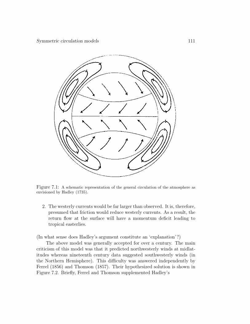
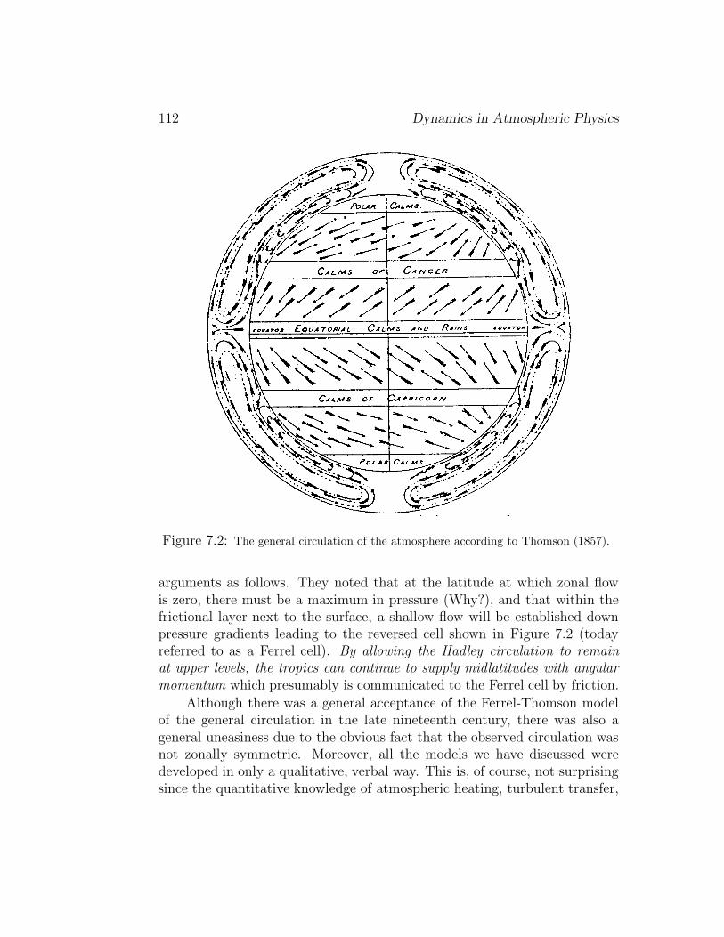
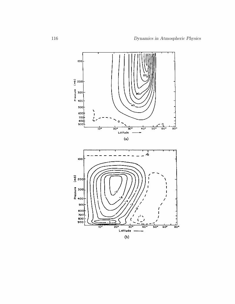
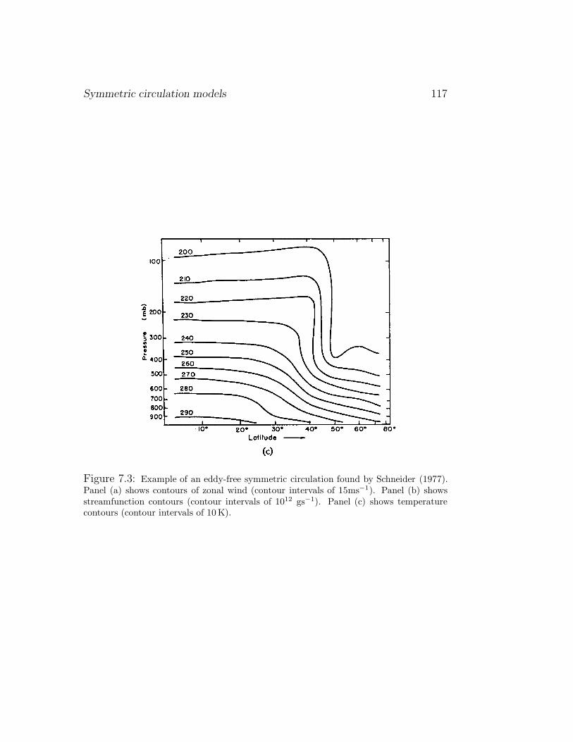
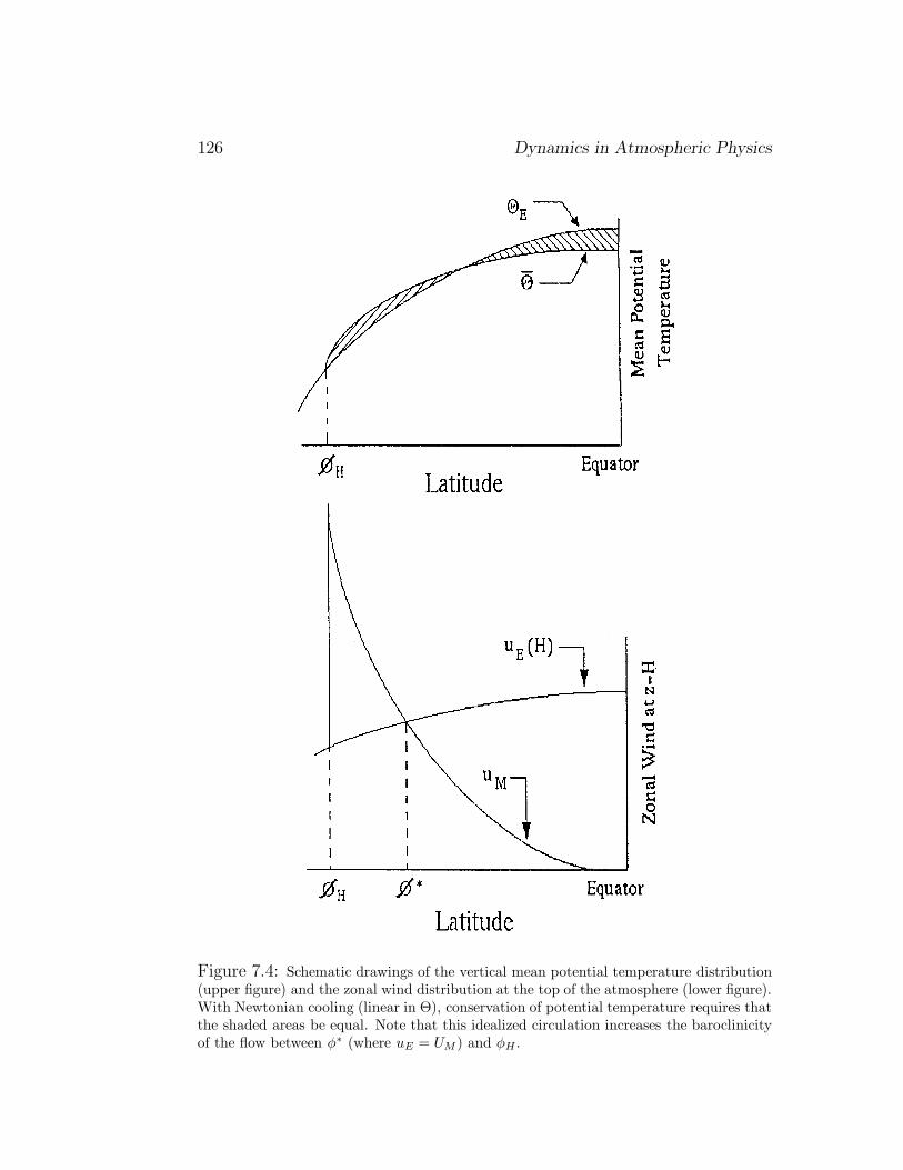
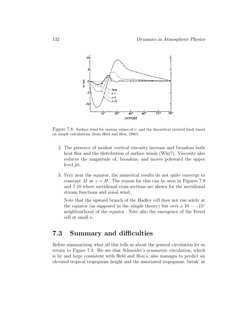
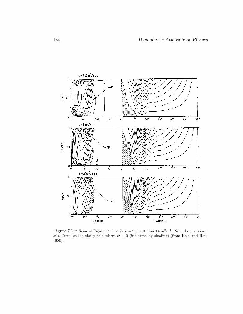
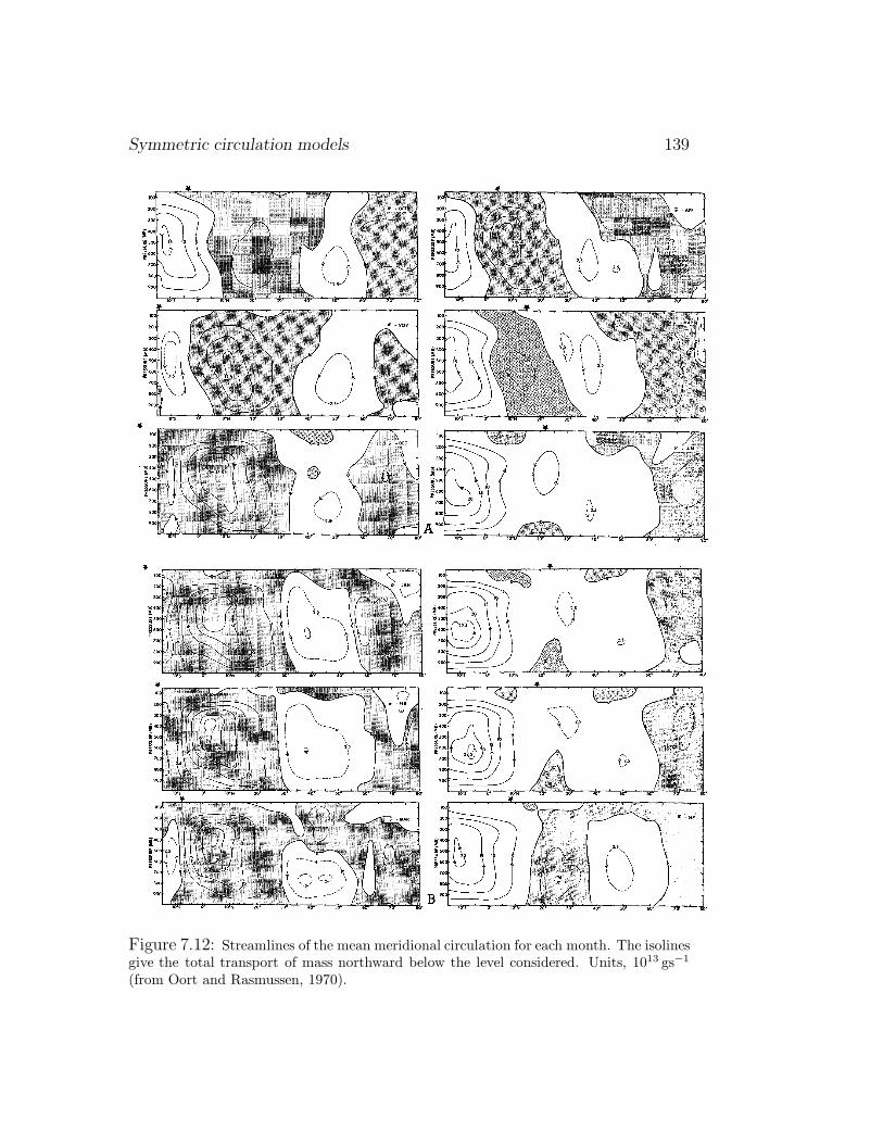
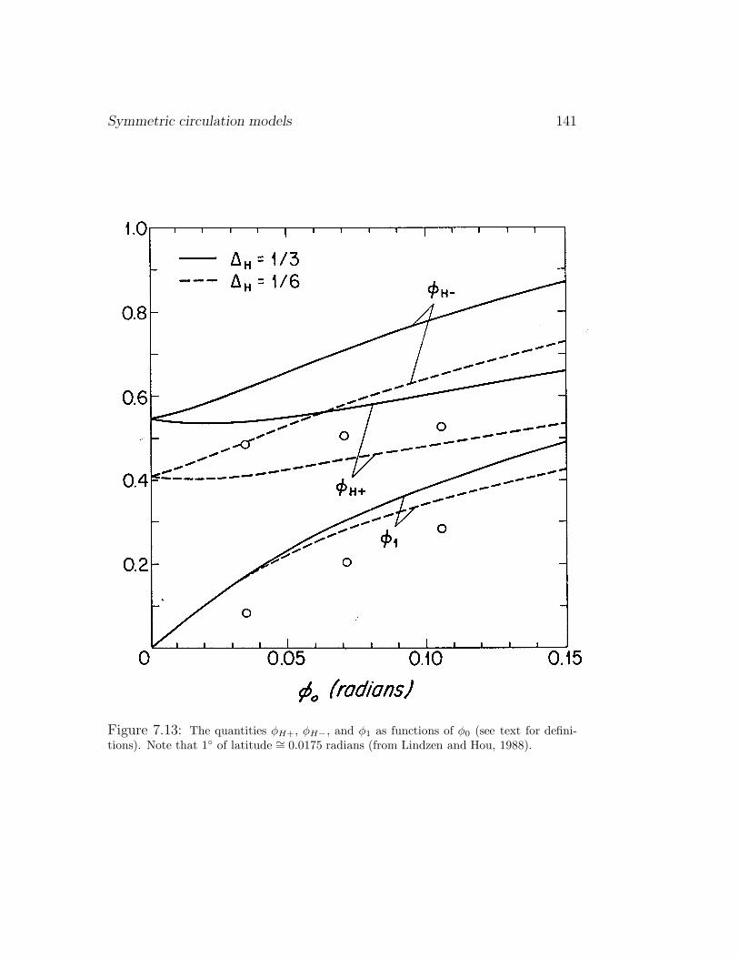Lorenz which are not universally agreed on but this hardly diminishes its value

There are several reasons for focussing on the zonally averaged circulashytion

1 Significant motion systems like the tropical tradewinds are well deshyscribed by zonal averages

2 The circulation of the atmosphere is only a small perturbation on a rigidly rotating basic state which is zonally symmetric

3 The zonally averaged circulation is a convenient subset of the total circulation

Our approach in this chapter will be to inquire how the atmosphere would behave in the absence of eddies It is hoped that a comparison of such results with observations will lend some insight into what maintains the observed zonally averaged state In particular discrepancies may point to the role of eddies in maintaining the zonal average This has been a matter of active controversy to the present

71 Historical review

A very complete historical treatment of this subject is given in chapter 4 of Lorenz We will only present a limited sketch here The first treatment of contemporary relevance was that of Hadley (1735) Hadleyrsquos aim was to explain the easterly (actually northeasterly in the Northern Hemisphere) tradewinds of the tropics and the prevailing westerlies of middle latitudes His brief explanation is summarized in Figure 71 Ignoring Hadleyrsquos error in assuming conservation of velocity rather than angular momentum Hadleyrsquos argument ran roughly as follows

1 Warm air rises at the equator and flows poleward at upper levels apshyproximately conserving angular momentum (In view of the remarks at the end of Chapter 6 it is not however at all obvious why one would have a meridional circulaton at all We will discuss this later) Beshycause the distance from the axis of rotation diminishes with increasing latitude large westerly currents are produced at high latitudes














+ upartx

+ vparty

+ wpartz

minus a

+ a

1 partp 1 = minus




partt partx

that


a a



minus a

= a partφ

minus a

= a cosφ partφ

(u cosφ)

Thus (71) becomes

v part partu 1






partz partz








20 must be balanced













middot u = 0 (75)



v minus



partv


= minusa partφ

+ partz

νpartz

(77)

(uΘ) = part



minus τ

and partΦ Θ

= g (79) partz Θ0



ΘE(φ z)

1 2

H






no heat conduction



no stress

partΘ = w = 0 at z = 0 (712)

partz



v = 0 at φ = 0 (714)




v = w = 0 (715)

Θ = ΘE (716)

and

u = uE (717)

where uE satisfies


part

uE 2 tan φ

g partΘE

partz fuE +

a = minus



12

uE z = 1 + 2R minus 1 cos φ (719)

Ωa H

where

gHΔHR = (720)

(Ωa)2

When R 1









(723)



Mmax lt Ωa 2 (724)





cos φ





cosφlowast




For small R



g = 98 msminus2

H = 15 104 m

Ω = 2π(864 104 s)

a = 64 106 m

and

ΔH sim 13


R asymp 226

and

R12 asymp 48


and from (728)

φlowast asymp 30







In addition



Ωa sin2 φ u(H φ) = uM = (729)






a minusa partφ



a 1 part

= minusa partφ

[Φ(H) minus Φ(0)] (731)



g Θ (732)

H Θ0




(733) a

minusaΘ0 partφ






a sin4 φ (735)

Θ0 gH 2 cos2 φ







φH φH





Θ0 asymp

Θ0 minus

2 gH φ4 (738)

and (710) becomes


2 (739) Θ0 Θ0


Θ(0) ΘE(0) 5

Θ0 =

Θ0 minus

18 RΔH (740)

and

12

φH = R (741) 3

5








2





φ sim Rlowast14

where

τν

gH


ΔV





1 H 1 part




1 H

vΘ dz Θ0 0

5

512 HaΔH

⎡ φ

φ 3

φ 5⎤

=18 3 τ

R32 ⎣ φH

minus 2 φH

+ φH

⎦ (743)





Θ(H) minus Θ(0)




Θ0




1 H




H



1 part H



⎡ 2 4 6⎤



⎣ φH

minus 3 φH

+3 φH

⎦ (747)


312

φ lt φH (748) 7

and westerlies for

312






τ = 20 days

C = 0005 msminus1

ΔV = 18













































ΘE ΔH z 1

Θ0

sim3 H

minus2







































+ upartx

+ vparty

+ wpartz

minus a

+ a

1 partp 1 = minus




partt partx

that


a a



minus a

= a partφ

minus a

= a cosφ partφ

(u cosφ)

Thus (71) becomes

v part partu 1






partz partz








20 must be balanced













middot u = 0 (75)



v minus



partv


= minusa partφ

+ partz

νpartz

(77)

(uΘ) = part



minus τ

and partΦ Θ

= g (79) partz Θ0



ΘE(φ z)

1 2

H






no heat conduction



no stress

partΘ = w = 0 at z = 0 (712)

partz



v = 0 at φ = 0 (714)




v = w = 0 (715)

Θ = ΘE (716)

and

u = uE (717)

where uE satisfies


part

uE 2 tan φ

g partΘE

partz fuE +

a = minus



12

uE z = 1 + 2R minus 1 cos φ (719)

Ωa H

where

gHΔHR = (720)

(Ωa)2

When R 1









(723)



Mmax lt Ωa 2 (724)





cos φ





cosφlowast




For small R



g = 98 msminus2

H = 15 104 m

Ω = 2π(864 104 s)

a = 64 106 m

and

ΔH sim 13


R asymp 226

and

R12 asymp 48


and from (728)

φlowast asymp 30







In addition



Ωa sin2 φ u(H φ) = uM = (729)






a minusa partφ



a 1 part

= minusa partφ

[Φ(H) minus Φ(0)] (731)



g Θ (732)

H Θ0




(733) a

minusaΘ0 partφ






a sin4 φ (735)

Θ0 gH 2 cos2 φ







φH φH





Θ0 asymp

Θ0 minus

2 gH φ4 (738)

and (710) becomes


2 (739) Θ0 Θ0


Θ(0) ΘE(0) 5

Θ0 =

Θ0 minus

18 RΔH (740)

and

12

φH = R (741) 3

5








2





φ sim Rlowast14

where

τν

gH


ΔV





1 H 1 part




1 H

vΘ dz Θ0 0

5

512 HaΔH

⎡ φ

φ 3

φ 5⎤

=18 3 τ

R32 ⎣ φH

minus 2 φH

+ φH

⎦ (743)





Θ(H) minus Θ(0)




Θ0




1 H




H



1 part H



⎡ 2 4 6⎤



⎣ φH

minus 3 φH

+3 φH

⎦ (747)


312

φ lt φH (748) 7

and westerlies for

312






τ = 20 days

C = 0005 msminus1

ΔV = 18













































ΘE ΔH z 1

Θ0

sim3 H

minus2






























20 must be balanced













middot u = 0 (75)



v minus



partv


= minusa partφ

+ partz

νpartz

(77)

(uΘ) = part



minus τ

and partΦ Θ

= g (79) partz Θ0



ΘE(φ z)

1 2

H






no heat conduction



no stress

partΘ = w = 0 at z = 0 (712)

partz



v = 0 at φ = 0 (714)




v = w = 0 (715)

Θ = ΘE (716)

and

u = uE (717)

where uE satisfies


part

uE 2 tan φ

g partΘE

partz fuE +

a = minus



12

uE z = 1 + 2R minus 1 cos φ (719)

Ωa H

where

gHΔHR = (720)

(Ωa)2

When R 1









(723)



Mmax lt Ωa 2 (724)





cos φ





cosφlowast




For small R



g = 98 msminus2

H = 15 104 m

Ω = 2π(864 104 s)

a = 64 106 m

and

ΔH sim 13


R asymp 226

and

R12 asymp 48


and from (728)

φlowast asymp 30







In addition



Ωa sin2 φ u(H φ) = uM = (729)






a minusa partφ



a 1 part

= minusa partφ

[Φ(H) minus Φ(0)] (731)



g Θ (732)

H Θ0




(733) a

minusaΘ0 partφ






a sin4 φ (735)

Θ0 gH 2 cos2 φ







φH φH





Θ0 asymp

Θ0 minus

2 gH φ4 (738)

and (710) becomes


2 (739) Θ0 Θ0


Θ(0) ΘE(0) 5

Θ0 =

Θ0 minus

18 RΔH (740)

and

12

φH = R (741) 3

5








2





φ sim Rlowast14

where

τν

gH


ΔV





1 H 1 part




1 H

vΘ dz Θ0 0

5

512 HaΔH

⎡ φ

φ 3

φ 5⎤

=18 3 τ

R32 ⎣ φH

minus 2 φH

+ φH

⎦ (743)





Θ(H) minus Θ(0)




Θ0




1 H




H



1 part H



⎡ 2 4 6⎤



⎣ φH

minus 3 φH

+3 φH

⎦ (747)


312

φ lt φH (748) 7

and westerlies for

312






τ = 20 days

C = 0005 msminus1

ΔV = 18













































ΘE ΔH z 1

Θ0

sim3 H

minus2


































middot u = 0 (75)



v minus



partv


= minusa partφ

+ partz

νpartz

(77)

(uΘ) = part



minus τ

and partΦ Θ

= g (79) partz Θ0



ΘE(φ z)

1 2

H






no heat conduction



no stress

partΘ = w = 0 at z = 0 (712)

partz



v = 0 at φ = 0 (714)




v = w = 0 (715)

Θ = ΘE (716)

and

u = uE (717)

where uE satisfies


part

uE 2 tan φ

g partΘE

partz fuE +

a = minus



12

uE z = 1 + 2R minus 1 cos φ (719)

Ωa H

where

gHΔHR = (720)

(Ωa)2

When R 1









(723)



Mmax lt Ωa 2 (724)





cos φ





cosφlowast




For small R



g = 98 msminus2

H = 15 104 m

Ω = 2π(864 104 s)

a = 64 106 m

and

ΔH sim 13


R asymp 226

and

R12 asymp 48


and from (728)

φlowast asymp 30







In addition



Ωa sin2 φ u(H φ) = uM = (729)






a minusa partφ



a 1 part

= minusa partφ

[Φ(H) minus Φ(0)] (731)



g Θ (732)

H Θ0




(733) a

minusaΘ0 partφ






a sin4 φ (735)

Θ0 gH 2 cos2 φ







φH φH





Θ0 asymp

Θ0 minus

2 gH φ4 (738)

and (710) becomes


2 (739) Θ0 Θ0


Θ(0) ΘE(0) 5

Θ0 =

Θ0 minus

18 RΔH (740)

and

12

φH = R (741) 3

5








2





φ sim Rlowast14

where

τν

gH


ΔV





1 H 1 part




1 H

vΘ dz Θ0 0

5

512 HaΔH

⎡ φ

φ 3

φ 5⎤

=18 3 τ

R32 ⎣ φH

minus 2 φH

+ φH

⎦ (743)





Θ(H) minus Θ(0)




Θ0




1 H




H



1 part H



⎡ 2 4 6⎤



⎣ φH

minus 3 φH

+3 φH

⎦ (747)


312

φ lt φH (748) 7

and westerlies for

312






τ = 20 days

C = 0005 msminus1

ΔV = 18













































ΘE ΔH z 1

Θ0

sim3 H

minus2




























no heat conduction



no stress

partΘ = w = 0 at z = 0 (712)

partz



v = 0 at φ = 0 (714)




v = w = 0 (715)

Θ = ΘE (716)

and

u = uE (717)

where uE satisfies


part

uE 2 tan φ

g partΘE

partz fuE +

a = minus



12

uE z = 1 + 2R minus 1 cos φ (719)

Ωa H

where

gHΔHR = (720)

(Ωa)2

When R 1









(723)



Mmax lt Ωa 2 (724)





cos φ





cosφlowast




For small R



g = 98 msminus2

H = 15 104 m

Ω = 2π(864 104 s)

a = 64 106 m

and

ΔH sim 13


R asymp 226

and

R12 asymp 48


and from (728)

φlowast asymp 30







In addition



Ωa sin2 φ u(H φ) = uM = (729)






a minusa partφ



a 1 part

= minusa partφ

[Φ(H) minus Φ(0)] (731)



g Θ (732)

H Θ0




(733) a

minusaΘ0 partφ






a sin4 φ (735)

Θ0 gH 2 cos2 φ







φH φH





Θ0 asymp

Θ0 minus

2 gH φ4 (738)

and (710) becomes


2 (739) Θ0 Θ0


Θ(0) ΘE(0) 5

Θ0 =

Θ0 minus

18 RΔH (740)

and

12

φH = R (741) 3

5








2





φ sim Rlowast14

where

τν

gH


ΔV





1 H 1 part




1 H

vΘ dz Θ0 0

5

512 HaΔH

⎡ φ

φ 3

φ 5⎤

=18 3 τ

R32 ⎣ φH

minus 2 φH

+ φH

⎦ (743)





Θ(H) minus Θ(0)




Θ0




1 H




H



1 part H



⎡ 2 4 6⎤



⎣ φH

minus 3 φH

+3 φH

⎦ (747)


312

φ lt φH (748) 7

and westerlies for

312






τ = 20 days

C = 0005 msminus1

ΔV = 18













































ΘE ΔH z 1

Θ0

sim3 H

minus2



























part

uE 2 tan φ

g partΘE

partz fuE +

a = minus



12

uE z = 1 + 2R minus 1 cos φ (719)

Ωa H

where

gHΔHR = (720)

(Ωa)2

When R 1









(723)



Mmax lt Ωa 2 (724)





cos φ





cosφlowast




For small R



g = 98 msminus2

H = 15 104 m

Ω = 2π(864 104 s)

a = 64 106 m

and

ΔH sim 13


R asymp 226

and

R12 asymp 48


and from (728)

φlowast asymp 30







In addition



Ωa sin2 φ u(H φ) = uM = (729)






a minusa partφ



a 1 part

= minusa partφ

[Φ(H) minus Φ(0)] (731)



g Θ (732)

H Θ0




(733) a

minusaΘ0 partφ






a sin4 φ (735)

Θ0 gH 2 cos2 φ







φH φH





Θ0 asymp

Θ0 minus

2 gH φ4 (738)

and (710) becomes


2 (739) Θ0 Θ0


Θ(0) ΘE(0) 5

Θ0 =

Θ0 minus

18 RΔH (740)

and

12

φH = R (741) 3

5








2





φ sim Rlowast14

where

τν

gH


ΔV





1 H 1 part




1 H

vΘ dz Θ0 0

5

512 HaΔH

⎡ φ

φ 3

φ 5⎤

=18 3 τ

R32 ⎣ φH

minus 2 φH

+ φH

⎦ (743)





Θ(H) minus Θ(0)




Θ0




1 H




H



1 part H



⎡ 2 4 6⎤



⎣ φH

minus 3 φH

+3 φH

⎦ (747)


312

φ lt φH (748) 7

and westerlies for

312






τ = 20 days

C = 0005 msminus1

ΔV = 18













































ΘE ΔH z 1

Θ0

sim3 H

minus2




























Mmax lt Ωa 2 (724)





cos φ





cosφlowast




For small R



g = 98 msminus2

H = 15 104 m

Ω = 2π(864 104 s)

a = 64 106 m

and

ΔH sim 13


R asymp 226

and

R12 asymp 48


and from (728)

φlowast asymp 30







In addition



Ωa sin2 φ u(H φ) = uM = (729)






a minusa partφ



a 1 part

= minusa partφ

[Φ(H) minus Φ(0)] (731)



g Θ (732)

H Θ0




(733) a

minusaΘ0 partφ






a sin4 φ (735)

Θ0 gH 2 cos2 φ







φH φH





Θ0 asymp

Θ0 minus

2 gH φ4 (738)

and (710) becomes


2 (739) Θ0 Θ0


Θ(0) ΘE(0) 5

Θ0 =

Θ0 minus

18 RΔH (740)

and

12

φH = R (741) 3

5








2





φ sim Rlowast14

where

τν

gH


ΔV





1 H 1 part




1 H

vΘ dz Θ0 0

5

512 HaΔH

⎡ φ

φ 3

φ 5⎤

=18 3 τ

R32 ⎣ φH

minus 2 φH

+ φH

⎦ (743)





Θ(H) minus Θ(0)




Θ0




1 H




H



1 part H



⎡ 2 4 6⎤



⎣ φH

minus 3 φH

+3 φH

⎦ (747)


312

φ lt φH (748) 7

and westerlies for

312






τ = 20 days

C = 0005 msminus1

ΔV = 18













































ΘE ΔH z 1

Θ0

sim3 H

minus2





























cosφlowast




For small R



g = 98 msminus2

H = 15 104 m

Ω = 2π(864 104 s)

a = 64 106 m

and

ΔH sim 13


R asymp 226

and

R12 asymp 48


and from (728)

φlowast asymp 30







In addition



Ωa sin2 φ u(H φ) = uM = (729)






a minusa partφ



a 1 part

= minusa partφ

[Φ(H) minus Φ(0)] (731)



g Θ (732)

H Θ0




(733) a

minusaΘ0 partφ






a sin4 φ (735)

Θ0 gH 2 cos2 φ







φH φH





Θ0 asymp

Θ0 minus

2 gH φ4 (738)

and (710) becomes


2 (739) Θ0 Θ0


Θ(0) ΘE(0) 5

Θ0 =

Θ0 minus

18 RΔH (740)

and

12

φH = R (741) 3

5








2





φ sim Rlowast14

where

τν

gH


ΔV





1 H 1 part




1 H

vΘ dz Θ0 0

5

512 HaΔH

⎡ φ

φ 3

φ 5⎤

=18 3 τ

R32 ⎣ φH

minus 2 φH

+ φH

⎦ (743)





Θ(H) minus Θ(0)




Θ0




1 H




H



1 part H



⎡ 2 4 6⎤



⎣ φH

minus 3 φH

+3 φH

⎦ (747)


312

φ lt φH (748) 7

and westerlies for

312






τ = 20 days

C = 0005 msminus1

ΔV = 18













































ΘE ΔH z 1

Θ0

sim3 H

minus2



























and from (728)

φlowast asymp 30







In addition



Ωa sin2 φ u(H φ) = uM = (729)






a minusa partφ



a 1 part

= minusa partφ

[Φ(H) minus Φ(0)] (731)



g Θ (732)

H Θ0




(733) a

minusaΘ0 partφ






a sin4 φ (735)

Θ0 gH 2 cos2 φ







φH φH





Θ0 asymp

Θ0 minus

2 gH φ4 (738)

and (710) becomes


2 (739) Θ0 Θ0


Θ(0) ΘE(0) 5

Θ0 =

Θ0 minus

18 RΔH (740)

and

12

φH = R (741) 3

5








2





φ sim Rlowast14

where

τν

gH


ΔV





1 H 1 part




1 H

vΘ dz Θ0 0

5

512 HaΔH

⎡ φ

φ 3

φ 5⎤

=18 3 τ

R32 ⎣ φH

minus 2 φH

+ φH

⎦ (743)





Θ(H) minus Θ(0)




Θ0




1 H




H



1 part H



⎡ 2 4 6⎤



⎣ φH

minus 3 φH

+3 φH

⎦ (747)


312

φ lt φH (748) 7

and westerlies for

312






τ = 20 days

C = 0005 msminus1

ΔV = 18













































ΘE ΔH z 1

Θ0

sim3 H

minus2





























a minusa partφ



a 1 part

= minusa partφ

[Φ(H) minus Φ(0)] (731)



g Θ (732)

H Θ0




(733) a

minusaΘ0 partφ






a sin4 φ (735)

Θ0 gH 2 cos2 φ







φH φH





Θ0 asymp

Θ0 minus

2 gH φ4 (738)

and (710) becomes


2 (739) Θ0 Θ0


Θ(0) ΘE(0) 5

Θ0 =

Θ0 minus

18 RΔH (740)

and

12

φH = R (741) 3

5








2





φ sim Rlowast14

where

τν

gH


ΔV





1 H 1 part




1 H

vΘ dz Θ0 0

5

512 HaΔH

⎡ φ

φ 3

φ 5⎤

=18 3 τ

R32 ⎣ φH

minus 2 φH

+ φH

⎦ (743)





Θ(H) minus Θ(0)




Θ0




1 H




H



1 part H



⎡ 2 4 6⎤



⎣ φH

minus 3 φH

+3 φH

⎦ (747)


312

φ lt φH (748) 7

and westerlies for

312






τ = 20 days

C = 0005 msminus1

ΔV = 18













































ΘE ΔH z 1

Θ0

sim3 H

minus2






























φH φH





Θ0 asymp

Θ0 minus

2 gH φ4 (738)

and (710) becomes


2 (739) Θ0 Θ0


Θ(0) ΘE(0) 5

Θ0 =

Θ0 minus

18 RΔH (740)

and

12

φH = R (741) 3

5








2





φ sim Rlowast14

where

τν

gH


ΔV





1 H 1 part




1 H

vΘ dz Θ0 0

5

512 HaΔH

⎡ φ

φ 3

φ 5⎤

=18 3 τ

R32 ⎣ φH

minus 2 φH

+ φH

⎦ (743)





Θ(H) minus Θ(0)




Θ0




1 H




H



1 part H



⎡ 2 4 6⎤



⎣ φH

minus 3 φH

+3 φH

⎦ (747)


312

φ lt φH (748) 7

and westerlies for

312






τ = 20 days

C = 0005 msminus1

ΔV = 18













































ΘE ΔH z 1

Θ0

sim3 H

minus2

































2





φ sim Rlowast14

where

τν

gH


ΔV





1 H 1 part




1 H

vΘ dz Θ0 0

5

512 HaΔH

⎡ φ

φ 3

φ 5⎤

=18 3 τ

R32 ⎣ φH

minus 2 φH

+ φH

⎦ (743)





Θ(H) minus Θ(0)




Θ0




1 H




H



1 part H



⎡ 2 4 6⎤



⎣ φH

minus 3 φH

+3 φH

⎦ (747)


312

φ lt φH (748) 7

and westerlies for

312






τ = 20 days

C = 0005 msminus1

ΔV = 18













































ΘE ΔH z 1

Θ0

sim3 H

minus2




























1 H 1 part




1 H

vΘ dz Θ0 0

5

512 HaΔH

⎡ φ

φ 3

φ 5⎤

=18 3 τ

R32 ⎣ φH

minus 2 φH

+ φH

⎦ (743)





Θ(H) minus Θ(0)




Θ0




1 H




H



1 part H



⎡ 2 4 6⎤



⎣ φH

minus 3 φH

+3 φH

⎦ (747)


312

φ lt φH (748) 7

and westerlies for

312






τ = 20 days

C = 0005 msminus1

ΔV = 18













































ΘE ΔH z 1

Θ0

sim3 H

minus2



























1 H




H



1 part H



⎡ 2 4 6⎤



⎣ φH

minus 3 φH

+3 φH

⎦ (747)


312

φ lt φH (748) 7

and westerlies for

312






τ = 20 days

C = 0005 msminus1

ΔV = 18













































ΘE ΔH z 1

Θ0

sim3 H

minus2





























τ = 20 days

C = 0005 msminus1

ΔV = 18













































ΘE ΔH z 1

Θ0

sim3 H

minus2



































































ΘE ΔH z 1

Θ0

sim3 H

minus2


























Chapter 7 Symmetric circulation models - MIT OpenCourseWare · Symmetric circulation models 111...

Documents

Transcript of Chapter 7 Symmetric circulation models - MIT OpenCourseWare · Symmetric circulation models 111...