CHAPTER 7 perpetual system and conceptually … 7 Inventories and Cost of Goods Sold 303 7-30 There...

298

CHAPTER 7

7-1 Sales transactions are accompanied by recording of the cost of goods sold (or cost of sales). This is literally true under the perpetual system and conceptually descriptive under the periodic system.

7-2 The two steps are obtaining (1) a physical count and (2) a cost

valuation. 7-3 Perpetual systems provide continuous inventory and cost of

goods sold records. Periodic systems rely on physical inventory taking to record cost of goods sold at the end of the period.

7-4 It is true that the periodic method requires a physical count to

measure cost of goods sold and the perpetual method does not. However, for control purposes, it is important to undertake at least annual physical counts of inventory under the perpetual method, as well.

7-5 F.O.B. destination means the shipper pays the freight bill.

F.O.B shipping point means the customer bears the cost of the freight bill. F.O.B. stands for "free on board."

7-6 Freight out is not shown as a direct offset to sales. Unlike sales

discounts and returns, freight out is not a part of gross revenue that never gets collected. Instead, it is an expense, entailing ordinary cash disbursements.

Chapter 7 Inventories and Cost of Goods Sold 299

7-7 The four methods are: 1. Specific identification – charges the actual cost of the

specific item sold. 2. FIFO – items purchased first are assumed to be sold first. 3. LIFO – items purchased most recently are assumed to be

sold first. 4. Weighted average – the average cost of all items

available is charged for each item sold. 7-8 The specific identification method is normally used for low

volume, high value items. Therefore, we would expect this to be used for a, b, d, and f.

7-9 Yes. Under FIFO the oldest costs are assigned to the cost of

goods sold first, so the timing of purchases cannot affect cost flows.

7-10 The good news is that LIFO reduces taxes in times of rising

prices. The bad news is that reported profit is lower. 7-11 Yes. Purchases under LIFO can affect income immediately,

because the unit costs of the latest purchases are assigned to units sold.

7-12 No. The weighted average must take into account the number

of units purchased at each price. For Gamma Company, the weighted average unit cost of inventory is: [(2 x $4.00) + (3 x $5.00)] ÷ 5 = $4.60.

7-13 Ending inventory is lower under LIFO in a period of rising prices

and constant or growing inventory. FIFO produces the higher ending inventory value.

300

7-14 Falling prices reverse the normal relation, so FIFO produces higher cost of goods sold and, therefore, lower net earnings. This helps explain why computer and electronics firms typically use FIFO in order to lower their taxes.

7-15 Consistency requires the maintaining of constant accounting

methods from period to period. Switching accounting methods hinders comparisons of current results to those of preceding periods.

7-16 Companies have adopted LIFO primarily because it saves

income taxes during times of rising prices by reporting higher cost of goods sold and lower profits.

7-17 An inventory profit is fictitious because, for a going concern, it

represents an amount necessary for replenishing inventory and is therefore not "available" in the form of cash for distribution as dividends. It arose from change in unit costs of the products purchased, not from the company's value added activities.

7-18 LIFO inventory valuations can be absurd because inventory

valuation is based on older and older costs as the years pass. 7-19 Conservatism does result in lower immediate profits, but higher

profits are then shown in later periods. 7-20 This convention is called conservatism.


7-21 "Market" generally means cost of replacement at the date of the physical inventory.

7-22 The inconsistency is the willingness of accountants to have

replacement costs used as a basis for write-downs below historical costs, even though a market exchange has not occurred, but their unwillingness to have replacement costs used as a basis for write-ups above historical costs.

7-23 Many inventory errors do counterbalance. For example, an

ending inventory that is overstated will overstate current income. But the same overstated inventory becomes the beginning inventory the next year; hence, next year's income will be understated. To show this you might use the following schematic:

Year 1 Year 2

BI OK Too Large + Purchase OK OK Goods Available OK Too Large –Ending Inventory Too Large OK Cost of Goods Sold Too Small Too Large

This exercise stresses the fact that the ending inventory of one year becomes the beginning inventory of the subsequent year and the errors correct themselves.

7-24 Cost of goods sold = Beginning inventory + Purchases –

Ending inventory. 7-25 Past gross profit percentages are sometimes applied to

current revenue as interim estimates of gross profit for a month or quarter. Thus, the time and cost of taking physical inventories can be saved.

302

7-26 Grocery stores have a low profit margin. If the profit margin is 2%, a savings of $100 in shrinkage would be equivalent to a $5,000 increase in sales.

7-27 Your boss has a point. This is a cost benefit question. If we do

not give the discount, we may lose customers to competitors of ours that treat them better. But if it is not currently a custom in the industry, you may not have to do it. If offering the discount does not cause customers to buy more, it is giving money away. However, if it is not an industry custom and it attracts new customers, that may lead to a different conclusion. Compare how much your operating income would rise from newly attracted customers versus the discounts received by existing customers.

7-28 Phar Mor overstated its assets by overstating inventories. This

means that either liabilities or stockholders’ equity must also be overstated (to keep the balance sheet equation in balance). Most likely Phar Mor used a periodic inventory method, so that overstating ending inventory would reduce cost of goods sold and increase pretax profit. If the company used a perpetual inventory system, management must have made inappropriate credits to cost of goods sold or some other expense account to offset the additional debits to the inventory account.

7-29 Under the FIFO method, the cost of sales will be based on old

acquisition costs. Under the LIFO method, the cost of sales will be based on the most recent acquisition costs. Thus, under LIFO, if additional units are acquired on the last day of the year, the cost of those units will be included in cost of sales. Thus, under LIFO, additional purchases would produce higher cost of goods sold in this instance and lower evaluations for the purchasing officer. Thus, under LIFO he would be less likely to purchase additional oil on the last day of the year.


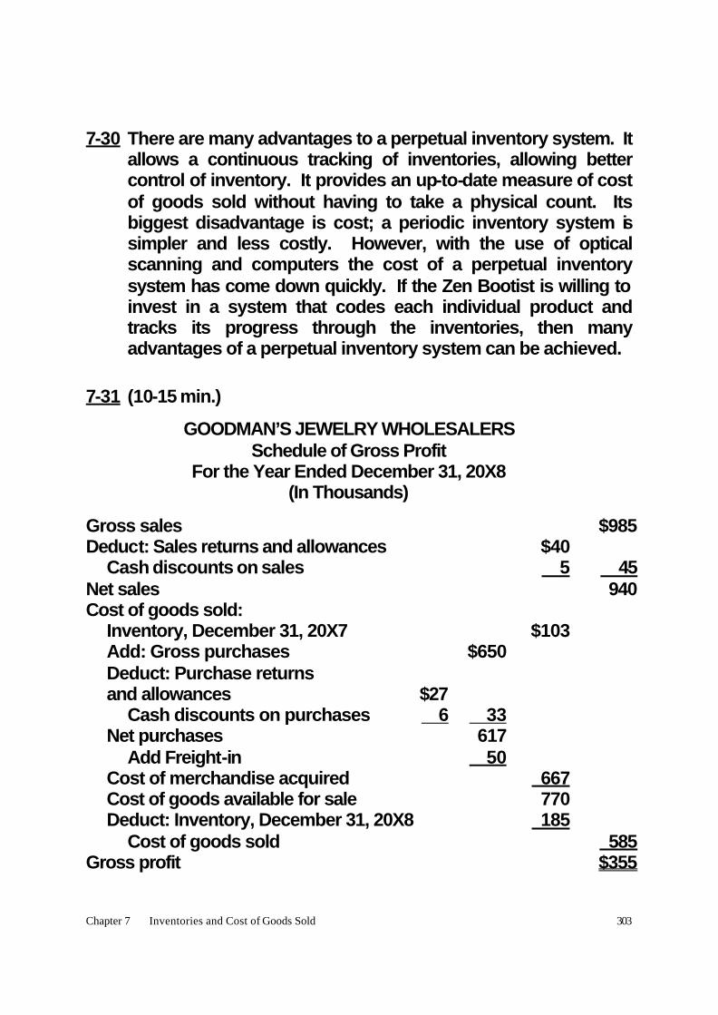
7-30 There are many advantages to a perpetual inventory system. It allows a continuous tracking of inventories, allowing better control of inventory. It provides an up-to-date measure of cost of goods sold without having to take a physical count. Its biggest disadvantage is cost; a periodic inventory system is simpler and less costly. However, with the use of optical scanning and computers the cost of a perpetual inventory system has come down quickly. If the Zen Bootist is willing to invest in a system that codes each individual product and tracks its progress through the inventories, then many advantages of a perpetual inventory system can be achieved.

7-31 (10-15 min.)

GOODMAN’S JEWELRY WHOLESALERS Schedule of Gross Profit For the Year Ended December 31, 20X8 (In Thousands)

Gross sales $985 Deduct: Sales returns and allowances $40 Cash discounts on sales 5 45 Net sales 940 Cost of goods sold: Inventory, December 31, 20X7 $103 Add: Gross purchases $650 Deduct: Purchase returns and allowances $27 Cash discounts on purchases 6 33 Net purchases 617 Add Freight-in 50 Cost of merchandise acquired 667 Cost of goods available for sale 770 Deduct: Inventory, December 31, 20X8 185 Cost of goods sold 585 Gross profit $355

304

7-32 (20 min.)

Sales $71,200 Sales returns 2,300 Net sales $68,900 Cost of goods sold: Inventory, January 1* x = $39,864 Purchases $54,000 Purchase returns 2,000 Net purchases $52,000 Freight in 500 52,500 Cost of goods available for sale $92,364 Inventory, January 15 40,000 Cost of goods sold, .76 x $68,900 52,364 Gross margin, .24 x $68,900 $16,536 * $52,364 + $40,000 – 52,500 = $39, 864 or: Cost of goods sold (.76 x 68,900) $52,364 Cost of goods purchased 52,500 Inventory increase $ 136 Beginning Balance = Ending Balance + Change = $40,000 - $136 $39,864


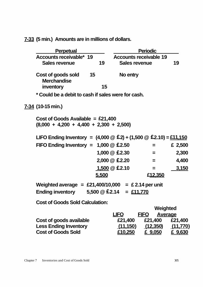
7-33 (5 min.) Amounts are in millions of dollars.

Perpetual Periodic Accounts receivable* 19 Accounts receivable 19 Sales revenue 19 Sales revenue 19 Cost of goods sold 15 No entry Merchandise inventory 15

* Could be a debit to cash if sales were for cash. 7-34 (10-15 min.) Cost of Goods Available = £21,400 (8,000 + 4,200 + 4,400 + 2,300 + 2,500) LIFO Ending Inventory = (4,000 @ £2) + (1,500 @ £2.10) = £11,150 FIFO Ending Inventory = 1,000 @ £2.50 = £ 2,500 1,000 @ £2.30 = 2,300 2,000 @ £2.20 = 4,400 1,500 @ £2.10 = 3,150 5,500 £12,350

Weighted average = £21,400/10,000 = £ 2.14 per unit Ending inventory 5,500 @ £2.14 = £11,770

Cost of Goods Sold Calculation: Weighted LIFO FIFO Average Cost of goods available £21,400 £21,400 £21,400 Less Ending Inventory (11,150) (12,350) (11,770) Cost of Goods Sold £10,250 £ 9,050 £ 9,630

306

7-35 (10-15 min.) This is straightforward. Answers are in Swiss francs.

Aug. 2 Purchases 350,000 Accounts payable 350,000 Aug. 3 Freight-in 15,000 Cash 15,000 Aug. 7 Accounts payable 30,000 Purchase returns and allowances 30,000 Aug. 11 Accounts payable 320,000 Cash discounts on purchases 6,400 Cash 313,600


7-36 (10-15 min.) 1. Invoice price $200,000 Add: Freight-in 10,000 Deduct: Purchase allowance (15,000) Deduct: Cash discount (3,700)* Total cost of steel acquired $191,300 *2% x ($200,000 – $15,000) 2. Purchases (or Inventory)* 200,000 Accounts payable 200,000

*The debit is to Purchases under the periodic inventory method and to Inventory under the perpetual inventory system.

Freight-in 10,000 Accounts payable (or cash) 10,000 Accounts payable 15,000 Purchase returns and allowances 15,000 Accounts payable 185,000 Cash discounts on purchases 3,700 Cash 181,300

308

7-37 (15 min.) Amounts are in thousands of dollars.

See Exhibit 7-37 for the balance sheet equation. Although not required, the balance sheet equation provides a good framework for understanding.

Journal Entries

Perpetual System a. Gross purchase: Inventory 960 Accounts payable 960

b. Returns and allowances: Accounts payable 80 Inventory 80

c. As goods are sold: Cost of goods sold 890 Inventory 890 d1. and d2. No entry Periodic System

a. Gross purchase: Purchases 960 Accounts payable 960

b. Returns and allowances: Accounts payable 80 Purchase returns and allowances 80

c. As goods are sold: No entry

d1. Transfer to cost of goods sold: Cost of goods sold 990 Purchase returns and allowances 80 Purchases 960 Inventory 110

d2. Recognize ending inventory: Inventory 100


Cost of goods sold 100

310

EXHIBIT 7-37 Entries are in thousands of dollars. A = L + SE Accounts Retained PERPETUAL SYSTEM Inventory Payable Earnings Balance, 12/31/X7 +110 = + 110 a. Gross purchases +960 = + 960 b. Returns and allowances – 80 = – 80

c. As goods are sold –890 –890

Sold Goods ofCost Increase

Closing the accounts at end of period: d1. No entry d2. No entry ____ ____ Ending balances, 12/31/X8 +100 = +990 –890


EXHIBIT 7-37 (continued) A = L + SE Purchase Returns and Accounts Retained PERIODIC SYSTEM Inventory Purchases Allowances Payable Earnings Balance, 12/31/X7 +110 = + 110 a. Gross purchases +960 = + 960 b. Returns and allowances –80 = – 80 c. As goods are sold (no entry) Closing the accounts at end of period:

d1. Transfer to cost of goods sold–110 –960 +80 = – 990

Sold Goods ofCost Increase

d2. Recognize ending inventory +100 = + 100

Sold Goods ofCost Decrease

___ ___ ___ Ending balances, 12/31/X8 +100 0 0 = +990 – 890


7-38 (10 min.)

This is straightforward.

1. Purchases 880,000 Accounts payable 880,000

2. Accounts payable 50,000 Purchase returns and allowances 50,000

3. Freight-in 74,000 Cash 74,000

4. Accounts payable 830,000 Cash 812,000 Cash discounts on purchases 18,000 7-39 (10 min.)

The entries could be compounded.

Accounts receivable (or Cash) 1,250,000 Sales 1,250,000

Cost of goods sold 957,000 Purchase returns and allowances 50,000 Cash discounts on purchases 18,000 Purchases 880,000 Freight-in 74,000 Inventory 71,000

Inventory 120,000 Cost of goods sold 120,000

314

7-40 (10-15 min.) Compound entries could be prepared. (Amounts are in millions.) Purchases 130 Accounts payable 130

Accounts receivable 239 Sales 239

Sales returns and allowances 5 Accounts receivable 5

Accounts payable 6 Purchase returns and allowances 6

Freight-in 14 Cash 14

Accounts payable 124 Cash discounts on purchases 1 Cash 123

Cash 226 Cash discounts on sales 8 Accounts receivable 234

Cost of goods sold 162 Purchase returns and allowances 6 Cash discounts on purchases 1 Inventory 25 Purchases 130 Freight-in 14

Inventory 45 Cost of goods sold 45

Other expenses 80


Cash (or other accounts) 80 7-41 (5 min.) Amounts are in millions of dollars. Beginning inventory $ 45 Purchases 4,510 Cost of goods available 4,555 Ending inventory (56) Cost of goods sold $4,499

316

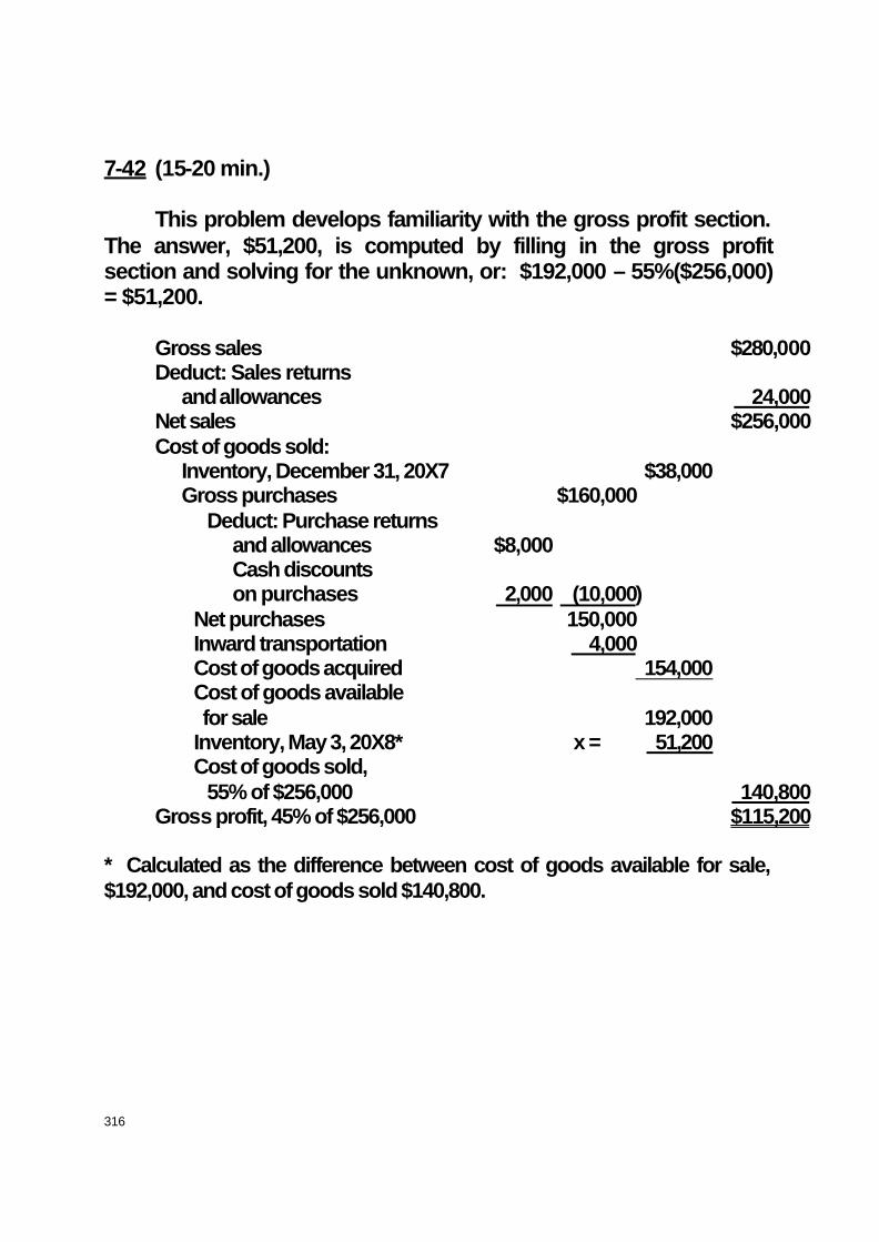
7-42 (15-20 min.) This problem develops familiarity with the gross profit section. The answer, $51,200, is computed by filling in the gross profit section and solving for the unknown, or: $192,000 – 55%($256,000) = $51,200.

Gross sales $280,000 Deduct: Sales returns and allowances 24,000 Net sales $256,000 Cost of goods sold: Inventory, December 31, 20X7 $38,000 Gross purchases $160,000 Deduct: Purchase returns and allowances $8,000 Cash discounts on purchases 2,000 (10,000) Net purchases 150,000 Inward transportation 4,000 Cost of goods acquired 154,000 Cost of goods available for sale 192,000 Inventory, May 3, 20X8* x = 51,200 Cost of goods sold, 55% of $256,000 140,800 Gross profit, 45% of $256,000 $115,200

* Calculated as the difference between cost of goods available for sale, $192,000, and cost of goods sold $140,800.


7-43 (15 min.)

Sales $200,000 Cost of goods sold: Inventory, January 1 $65,000 Purchases $195,000 Purchase returns and allowance 10,000 Net purchases $185,000 Freight-in 15,000 200,000 Cost of goods available for sale $265,000 Inventory, March 9* x = 105,000 Cost of goods sold, 80% of $200,000 160,000 Gross margin, 20% of $200,000 $ 40,000

* The answer, $105,000, is obtained by filling in the schedule of cost of goods sold and solving for the unknown, or: $265,000 – 80%($200,000) = $265,000 – $160,000 = $105,000. 7-44 (10-15 min.)

Beginning inventory $ 55,000 Purchases 200,000 Cost of goods available for sale $255,000 Less estimated cost of goods sold: 75%* of $280,000 210,000 Estimated ending inventory $ 45,000

*100% – 25% = 75%

The difference between $45,000 and the amount of inventory remaining is an estimate of the amount missing.

318

7-45 (10-15 min.) 1 & 2. To calculate the effect use the following approach: 20X5 20X6 Beginning inventory OK Too low $20,000 + Purchases OK OK Goods available OK Too low $20,000 −Ending inventory Too low $20,000 OK Cost-of-goods sold Too high $20,000 Too low $20,000 Cost-of-goods sold is too high by $20,000 in 20X5 so taxable income will be too low by $20,000. Taxes will be too low by $8,000 so net income and retained earnings will be too low by $12,000. Taxable income for 20X6 will be overstated by $20,000 and taxes will be $8,000 too high. Net income in 20X6 will be too high by $12,000 and retained earnings will be correct again at December 31, 20X6.


7-46 (10-15 min.) 1. Inventory turnover = cost of goods sold* ÷ average

inventory = $1,080,000 ÷ $1,080,000 = 1.00 *Cost of goods sold = $2,400,000 – $1,320,000 = $1,080,000 2. The gross profit would fall from $1,320,000 to $1,260,000, so a

change in pricing strategy would be undesirable for Custom Gems. The current 20X3 data follow:

Inventory turnover 1.0 Gross profit percentage: $1,320,000 ÷ $2,400,000 55% This percentage is not unusual. If prices are cut 20 percent in 20X4 without affecting inventory

turnover, new sales would be .8 x $2,400,000 = $1,920,000. Cost of goods sold on those sales would still be $1,080,000. Therefore Mr. Siegl would be reducing his gross profit from $1,320,000 to $1,920,000 - $1,080,000 = $840,000 and its gross profit percentage to 44% [($1,920,000 − $1,080,000) ÷ $1,920,000]. However, an increase in inventory turnover to 1.5 would produce the following:

Sales, $1,920,000 x 1.5 $2,880,000 Cost of goods sold, $1,080,000 x 1.5 1,620,000 Gross profit $1,260,000

Gross profit would be only $60,000 below the 20X3 level.

320

7-47 (15-20 min.) 1. LIFO Method: Inventory shows: 1,100 tons on hand at July 31. Costs: 1,000 tons @ $ 9.00 $ 9,000 100 tons @ $10.00 1,000 July 31 inventory cost. $10,000 FIFO Method: Inventory shows: 1,100 tons on hand at July 31. Costs: 900 tons @ $12.00 $10,800 200 tons @ $11.00 2,200 July 31 inventory cost. $13,000 2. Purchases: 5,000 tons @ $10 $50,000 1,000 tons @ $11 11,000 900 tons @ $12 10,800 Total purchases $71,800 Beginning inventory: 1,000 tons @ $ 9 9,000 LIFO FIFO Cost of goods available for sale $80,800 $ 80,800 $ 80,800 Less ending inventory (10,000) (13,000) Cost of goods sold $ 70,800 $ 67,800 Sales $102,000 $102,000 Cost of goods sold 70,800 67,800 Gross profit $ 31,200 $ 34,200


7-48 (5-10 min.)

The inventory would be written down from $200,000 to $185,000 on December 31, 20X1. The new $185,000 valuation is "what's left" of the original $200,000 cost. In other words, the $185,000 is the unexpired cost and may be thought of as the new cost of the inventory for future accounting purposes. Thus, because subsequent replacement values exceed the $185,000 cost, and write-ups above "cost" are not acceptable accounting practice, the valuation remains at $185,000 until it is written down to $180,000 on the following December 31, 20X2.

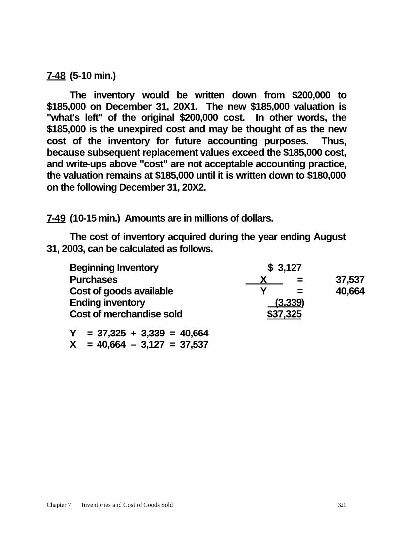
7-49 (10-15 min.) Amounts are in millions of dollars.

The cost of inventory acquired during the year ending August 31, 2003, can be calculated as follows.

Beginning Inventory $ 3,127 Purchases X = 37,537 Cost of goods available Y = 40,664 Ending inventory (3,339) Cost of merchandise sold $37,325

Y = 37,325 + 3,339 = 40,664 X = 40,664 – 3,127 = 37,537

322

7-50 (10 min.) Dollar amounts are in millions.

2003: ($11,305 − $7,799) ÷ $11,305 = 31.01% 2002: ($11,019 − $7,604) ÷ $11,019 = 30.99% 2001: ($11,332 − $7,815) ÷ $11,332 = 31.04%

The gross profit percentage was very steady over these three years, with just a slight dip in 2002 followed by a small recovery.

Though not in the problem, it might be interesting to note that the gross profit percentage has ranged for 27% to 31% over the past ten years. 7-51 (10-15 min.) 1. ISLAND BUILDING SUPPLY Statement of Gross Profit For the Year Ended December 31, 20X1

Sales $1,200,000Cost of goods sold: Inventory, beginning $ 240,000 Add net purchases 1,035,000 Cost of goods available for sale $1,275,000 Deduct ending inventory (330,000) Cost of goods sold 945,000 Gross profit $255,000

2. Inventory turnover = Cost of goods sold ÷ Average inventory = $945,000 ÷ [1/2 x (240,000 + 330,000)] = 945,000 ÷ 285,000 = 3.3 times


7-52 (30-40 min.) The detailed income statement is in the accompanying exhibit. Note the classification of operating expenses into a selling category and a general and administrative category. The list of accounts in the problem contained one item that belongs in a balance sheet rather than an income statement, the Allowance for Bad Debts (an offset to Accounts Receivable). The delivery expenses and the bad debts expense are shown under selling expenses. Some accountants prefer to show the bad debts expense as an offset to gross sales or as administrative expenses.

324

7-52 (continued)

BACKBAY BATHROOM SUPPLY COMPANY Income Statement For the Year Ended December 31, 20X5 (In Thousands)

Revenues: Gross sales $1,091 Deduct: Sales returns and allowances $ 50 Cash discounts on sales 16 66 Net sales $1,025Cost of goods sold: Inventory, December 31, 20X4 $200 Add purchases $600 Less: Purchase returns and allowances $40 Cash discounts on purchases 15 55 Net purchases $545 Add Freight in 50 Cost of merchandise acquired 595 Cost of goods available for sale $795 Deduct: Inventory, December 31, 20X5 300 Cost of goods sold 495 Gross profit from sales $ 530 Operating expenses: Selling expenses: Sales salaries and commissions $160 Rent expense, selling space 90 Advertising expense 45 Depreciation expense, trucks and store fixtures 29 Bad debts expense 8 Delivery expenses 20 Total selling expenses $352 General and administrative expenses: Office salaries 46 Rent expense, office space 10 Depreciation expense, office equipment 3 Office supplies used 6 Miscellaneous expenses 13 Total general and administrative expenses 78 Total operating expenses 430 Income before income tax $ 100 Income tax expense 42


Net income $ 58

326

7-53 (15-25 min.)

Under the FIFO cost-flow assumption, the periodic and perpetual procedures give identical results. The ending inventory will be valued on the basis of the last purchases during the period.

Units $ Beginning Inventory 120 600 Purchases 290 2,050 Goods available 410 2,650 Units sold 255 1,465** Units in ending Inventory 155 1,185*

* 155 units remain in ending inventory 100 will be valued at the $8 cost from the October 21 purchase and

the remaining 55 will be valued at the $7 cost from the May 9 purchase

100 x $8 = $ 800 55 x $7 = 385 $1,185 Ending inventory

** Reconciliation: Cost of Goods Sold: 255 Units: 120 x $5 = $ 600 80 x $6 = 480 55 x $7 = 385 $1,465


7-54 (30-35 min.) 1. Gross profit percentage = $1,600,000 ÷ $4,000,000 = 40%

Inventory turnover = $2,400,000 ÷ 2

750,000$850,000 +

= 3 times 2. Inventory turnover = $2,400,000 ÷ $600,000 = 4 times, a 1/3

increase in turnover. 3. With a lower average inventory and constant inventory

turnover, cost of sales must fall. Total cost of goods sold = $600,000 x 3 = $1,800,000. To achieve a gross profit of $1,600,000, total sales must be $1,800,000 + $1,600,000, or $3,400,000. The gross profit percentage must be $1,600,000 ÷ $3,400,000 = 47.1%. Requirements 2 & 3 show that if inventory levels are reduced you must increase either inventory turnover or margins to maintain profitability.

4. Summary (computations are shown below): Succeeding Year Given Year 4a 4b Sales $4,000,000 $3,857,143 $4,125,000 Cost of goods sold 2,400,000 2,160,000 2,640,000 Gross profit $1,600,000 $1,697,143 $1,485,000

328

7-54 (continued) a. New gross profit percentage, 40% + .10(40%) = 44% New inventory turnover, 3 – .10(3) = 2.7 New cost of goods sold, $800,000 x 2.7 = $2,160,000 New sales = $2,160,000 ÷ (1 – .44) = $2,160,000 ÷ .56 = $3,857,143

Note that this is a more profitable alternative, assuming that the gross profit percentage and the inventory turnover can be achieved. In contrast, alternative 4b is less attractive than the original 40% gross profit and turnover of 3.

b. New gross profit percentage, 40% – .10(40%) = 36% New inventory turnover, 3 + .10(3) = 3.3 New cost of goods sold, $800,000 x 3.3 = $2,640,000 New sales = $2,640,000 ÷ (1 −.36) = $2,640,000 ÷ .64 = $4,125,000 5. Retailers find these ratios (and variations thereof) helpful for a

variety of operating decisions, too many to enumerate here. An obvious help is the quantifying of the options facing management regarding what and how much inventory to carry, and what pricing policies to follow. You may want to stress that this analysis ignores one benefit of higher inventory turnover—the firm reduces its investment in inventory and reduces storage and display requirements.


7-55 (25-35 min.)

The detailed income statement is in the accompanying exhibit. Some accountants prefer to show the provision for uncollectible accounts as an offset to gross sales. The data for the allowance for doubtful accounts does not affect the income statement.

SEARS, ROEBUCK & COMPANY Income Statement For the Year Ended December 31, 2002 (In Millions)

Revenues: Gross revenues (Plug) $44,316 Deduct: Sales returns and allowances $ 2,100 Cash discounts on sales 850 2,950 Net revenues $41,366 Cost of goods sold: Inventory, December 31, 2001 $4,912 Add purchases $26,124 Less: Purchase returns and allowances $1,200 Cash discounts on purchases 180 1,380 Net purchases $24,744 Add Freight in 1,100 Cost of merchandise acquired 25,844 Cost of goods available for sale $30,756 Deduct: Inventory, December 31, 2002 5,115 Cost of sales 25,646 Gross profit $15,720 Operating expenses: Selling and administrative $9,249 Provision for uncollectible accounts 2,261 Depreciation 875 Other operating expenses 111 12,496 Operating income $ 3,224 Interest expense 1,143 Other income, net (372) Income before tax $ 2,453

330

7-56 (20-30 min.)

1. CONTRACTOR SUPPLY CO. Comparison of Inventory Methods Statement of Gross Profit of Kemtone Cooktops For the Year Ended December 31, 20X8 (In Dollars)

FIFO

LIFO Weighted Average

Sales, 260 units 26,200 26,200 26,200 Deduct cost of goods sold: Inventory, December 31,

20X7, 110 @ $50

5,500

5,500

5,500

Purchases, 300 units 21,200 21,200 21,200 Cost of goods available for

sale, 410 units

26,700

26,700

26,700

Deduct: Inventory, December 31, 20X8, 150 units:

100 @ $80 8,000 50 @ $70 3,500 11,500 110 @ $50 5,500 40 @ $60* 2,400 7,900 150 @ ($26,700 ÷ 410), 150 @ $65.12 9,768

Cost of goods sold, 260 units

15,200

18,800

16,932

Gross profit 11,000 7,400 9,268

* This is a periodic LIFO. Students are using perpetual LIFO if they answer 20 @ $60 plus 20 @ $80 = $2,800.

2. Income taxes would be lower by .40($11,000 – $7,400) = $1,440.

The income tax rate is assumed to be identical at all levels of taxable income. Some students will wonder why no information is given regarding other expenses and net income. Such information is unnecessary because other expenses, whatever their amounts, will be common among all inventory methods. Thus gross profits provide sufficient information to measure the differences in income taxes among various inventory methods.


7-57 (15-20 min.) There would be no effect on gross profit, net income, or income taxes under FIFO, although the balance sheet would show ending inventory as $8,000 higher. The income statement would show purchases and ending inventory as higher by $8,000, so the net effect on cost of goods sold would be zero. LIFO would show a lower gross profit, $6,000, as compared with $7,400, a decrease of $1,400. Hence, the impact of the late purchase on income taxes would be a savings of 40% of $1,400 = $560. The tabulation below compares the results under LIFO (in dollars):

Without Late Purchase With Late Purchase Sales, 260 Units 26,200 26,200 Deduct: Cost of goods sold: Inventory, December 31, 20X7, 110 @ $50

5,500

5,500

Purchases, 300 units at various costs

21,200

21,200

100 units @ $80 − 8,000 Cost of goods available for sale 26,700 34,700 Deduct: Inventory, December 31, 20X8:

First layer (pool) 110 @ $50 5,500 5,500 Second layer (pool) 40 @ $60 2,400 7,900 Second layer (pool) 80 @ $60 4,800 Third layer (pool) 60 @ $70 4,200 14,500 Cost of goods sold, 260 units 18,800 20,200 Gross profits 7,400 6,000 Income taxes @ 40% 2,960 2,400

332

7-57 (continued)

Although purchases are $8,000 higher than before, the new LIFO ending inventory is only $14,500 – $7,900 = $6,600 higher. The $1,400 difference in gross profit is explained by the fact that the late purchase resulted in changes to both ending inventory and cost of goods sold. LIFO cost of goods sold is $1,400 higher ($20,200 – $18,800). To see this from another angle, compare layers. Without the late purchase, the second layer had 40 units @ $60. With the late purchase: Late purchase released as expense, 100 @ $80 $8,000 Second layer is 40 units higher @ $60 = $2,400 Third layer is 60 units @ $70 = 4,200 Amount held as ending inventory that would otherwise have been released as expense in the form of cost of goods sold 6,600 Difference in cost of goods sold $1,400 7-58 (15 min.) 1. LIFO: 100 units @ $10 $1,000 20 units @ $12 240 $1,240 2. Replacement cost: 120 units @ $12 = $1,440. LIFO is lower than replacement cost. Therefore, no inventory

write-down takes place, and the balance sheet shows $1,240.

3. FIFO: 20 units @ $12 $ 240 100 units @ $13 1,300 $1,540

4. Replacement cost is $1,440 (see Requirement 2). Because replacement cost is lower than FIFO, the balance sheet should


include the lower amount, $1,440. Most companies would treat the $100 inventory write-down as an increase in cost of sales.

334

7-59 (10-15 min.)

1. O is used for overstated, U for understated, and N for not affected.

(In Thousands) 20X1 20X2

Beginning inventory* N O $15 Ending inventory* O $15 N Cost of goods sold U 15 O 15 Gross margin O 15 U 15 Income before income taxes O 15 U 15 Income tax expense O 6 U 6 Net income O 9 U 9

*The ending inventory for 20X1 becomes the beginning inventory for 20X2.

2. Retained earnings would be overstated by $9,000 at the end of the first year. However, the error would be offset in the second year, assuming no change in the 40% income tax rate. Therefore, retained earnings would be correct at the end of the second year.

7-60 (20-30 min.) 1. See Exhibit 7-60 on the following page. 2. LIFO results in more cash by the difference in income tax effects. LIFO

results in a lower cash outflow of .40 x ($116,000 – $96,000) = $8,000. 3. FIFO results in more cash when inventory prices are falling. Why?

Because income tax cash outflow would be more under LIFO by .40($144,000 – $124,000) = $8,000.


EXHIBIT 7-60 Purchases @ $12 Unit Purchases @ $8 Unit Requirement a Requirement b FIFO LIFO FIFO LIFO

Sales, 12,000 @ $20 $240,000 $240,000 $240,000$240,000 Deduct cost of goods sold: Inventory, December 31, 20X1, 10,000 @ $10 100,000 100,000 100,000 100,000 Purchases: 13,000 @ $12 and $8, respectively 156,000 156,000 104,000 104,000 Cost of goods available for sale 256,000 256,000 204,000 204,000 Deduct: Inventory, December 31, 20X2, 11,000 units: 11,000 @ $12 = 132,000 or 10,000 @ $10 = $100,000 1,000 @ $12 = 12,000 112,000 or 11,000 @ $ 8 = 88,000 or 10,000 @ $10 = $100,000 1,000 @ $ 8 = 8,000 108,000 Cost of goods sold 124,000 144,000 116,000 96,000 Gross margin $116,000 $ 96,000 $124,000$144,000

336

7-61 (20 min.) 1. Units LIFO FIFO

Sales 30,000 £330,000 £330,000 Cost of goods sold: Inventory, December 31, 20X7 14,000 84,000 84,000 Purchases 52,000 394,000 394,000 Cost of goods available for sale 66,000 478,000 478,000 Inventory, December 31, 20X8 36,000 238,000* 282,000** Cost of goods sold 30,000 240,000 196,000 Gross margin or gross profit £ 90,000 £134,000

* 14,000 @ £6 = £ 84,000 22,000 @ £7 = 154,000 36,000 £238,000 ** 30,000 @ £8 = £240,000 6,000 @ £7 = 42,000 36,000 £282,000

2. Gross margin is higher under FIFO. However, cash will be

higher under LIFO by .40(£134,000 – £90,000) = .40 x £44,000 = £17,600. Cash payments for inventory and cash receipts from sales are unaffected by the cost flow assumption. Only the effect on tax obligations affects cash flow.


7-62 (35 min.) 1. (Dollars In Thousands) Lastin Company Firstin Company (LIFO) (FIFO)

Sales $4,500 $4,500 Deduct cost of goods sold: Beginning inventory: 10,000 tons @ $50 $ 500 $ 500 Purchases: 30,000 tons @ $60 $1,800 20,000 tons @ $70 1,400 3,200 3,200 Cost of goods available for sale $3,700 $3,700 Ending inventory: 10,000 tons @ $50 $ 500 15,000 5,000 tons @ $60 300 800 @ $70 1,050 Cost of goods sold 2,900 2,650 Gross profit $1,600 $1,850 Other expenses 600 600 Income before income taxes $ 1,000 $1,250 Income taxes at 40% 400 500 Net income $ 600 $ 750

338

7-62 (continued) 2. Note first that the underlying events are identical, but the

inventory method chosen will yield radically different results. When prices are rising, and if she had a choice, the manager would choose the method that is most harmonious with her objectives. Clearly the company is better off economically under the LIFO method, even though reported earnings are less. LIFO saved $100 thousand in income taxes:

LIFO FIFO

Cash receipts: Sales $4,500 $4,500 Cash disbursements: Purchases $3,200 Other expenses 600 $3,800 $3,800 Income taxes 400 500 Total disbursements $4,200 $4,300 Net increase in cash $ 300 $ 200

On the other hand, reported net income is dramatically better under FIFO, $750 versus $600. In times of rising prices and stable or increasing inventory levels, the general guide is that LIFO saves income taxes and results in a better cash position; nevertheless, FIFO shows the higher reported net income.


7-63 (30 min.) 1. 20X1 20X2 20X3 20X4 20X5 Total FIFO: Sales $5,000 $5,000 $5,000 $5,000 $20,000 $40,000 Cost of goods sold 1,000 2,000 2,000 2,500 13,000 20,500 Income before taxes 4,000 3,000 3,000 2,500 7,000 19,500 Income taxes 1,600 1,200 1,200 1,000 2,800 7,800 Net income $2,400 $1,800 $1,800 $1,500 $ 4,200 $11,700 LIFO: Sales $5,000 $5,000 $5,000 $5,000 $20,000 $40,000 Cost of goods sold 2,000 2,500 3,000 4,000 9,000 20,500 Income before taxes 3,000 2,500 2,000 1,000 11,000 19,500 Income taxes 1,200 1,000 800 400 4,400 7,800 Net income $1,800 $1,500 $1,200$ 600 $ 6,600 $11,700 2. LIFO is most advantageous because it defers tax payments.

This provides additional cash and reduces the need for borrowing. One way to think about the benefit is to think of the interest saved each year. For example, assume that if higher taxes were paid, that amount would be borrowed at an interest rate of 10%.

20X1 20X2 20X3 20X4 20X5 Total

FIFO tax $1,600 $1,200 $1,200 $1,000 $2,800 $7,800 LIFO tax 1,200 1,000 800 400 4,400 7,800 Annual cash benefit /(loss) $ 400 $ 200 $ 400 $ 600 $(1,600)$ 0 Cumulative cash benefit $ 400 $ 600 $1,000 $1,600 – – Interest saved @ 10% $ 40 $ 60 $ 100 $ 160 – $ 360

This analysis does not consider the time value of money in that interest savings are simply added together, but it does provide a vivid illustration of the concept.

340

7-64 (30-40 min.) 1, 2. FIFO LIFO 1(a) 2(a) 1(b) 2(b) Sales, 5,000 units $120,000 $96,000 $120,000 $96,000 Less cost of goods sold: Purchase cost, $118,000 $118,000 Less ending inventory: FIFO: 4,000 @ $15 60,000 LIFO: 2,000 @ $10 = $20,000 1,000 @ $11 = 11,000 1,000 @ $13 = 13,000 44,000 Cost of goods sold $ 58,000 $60,000 $ 74,000 $44,000 Other expenses 30,000 30,000 30,000 30,000 Total deductions $ 88,000 $90,000 $104,000 $74,000 Income before taxes $ 32,000 $ 6,000 $ 16,000 $22,000 Income taxes @ 40% $ 12,800 $ 2,400 $ 6,400 $ 8,800 Net income $ 19,200 $ 3,600 $ 9,600 $13,200 3. FIFO LIFO 1(a) 2(a) 1(b) 2(b) Sales, 5,000 units $120,000 $96,000 $120,000 $96,000 Less cost of goods sold: Purchase cost* $ 58,000 $60,000 $ 58,000 $60,000 Other expenses 30,000 30,000 30,000 30,000 Total deductions $ 88,000 $90,000 $ 88,000 $90,000 Income before taxes $ 32,000 $ 6,000 $ 32,000 $ 6,000 Income taxes @ 40% $ 12,800 $ 2,400 $ 12,800 $ 2,400 Net income $ 19,200 $ 3,600 $ 19,200 $ 3,600 The timing of purchases does not affect FIFO income but affects LIFO income. LIFO cost of goods sold declined from $74,000 to $58,000 as a result of the delay in purchase. Managers can directly influence LIFO net income by choices to replenish inventory. * In this example all purchases are sold each year and no inventories

accumulate. Therefore, FIFO and LIFO give identical results.


7-65 (20-30 min.) The major point here is to demonstrate that changes in LIFO reserves can be used as a shortcut measure of the differences in cost of goods sold under FIFO and LIFO. (All amounts are in dollars.) LIFO 1. (1) (2) Reserve FIFO LIFO (1) – (2)

Beginning inventory, 2 @ $20, 2 @ $16 40 32 8 Purchases: 3 @ $24 + 3 @ $28 = 156 156 Cost of goods available for sale 196 188 8 Ending inventory, 2 @ $28, 2 @ $16 56 32 24 Cost of goods sold 140 156 (16)

2. a. Beginning inventory 40 32 8

Purchases (as above) 156 156 Cost of goods available for sale 196 188 8 Ending inventory 3 @ $28 + 1 @ $24 108 2 @ $16 + 2 @ $24 ___ 80 28 Cost of goods sold 88 108 (20)

b. Beginning inventory 40 32 8 Purchases 156 156 Available for sale 196 188 8 Ending inventory 0 0 0 Cost of goods sold 196 188 8

342

7-65 (continued) 3. From Part 1, the beginning LIFO Reserve is 8, the difference

between FIFO inventory of 40 and LIFO inventory of 32. At year end the LIFO Reserve is 24, an increase of 16. This 16 is exactly the difference between FIFO cost of goods sold of 140 and LIFO cost of goods sold of 156. If prices are rising, cost of goods sold includes more of these recent higher costs under LIFO than under FIFO. Hence, if physical quantities are held constant, the LIFO reserve will rise by the difference between the cost of goods sold. Why? Because old LIFO unit costs will still be held in ending inventory, whereas recent higher unit costs will apply to the ending FIFO inventory.

If physical quantities of ending inventory rise along with rises in

unit prices, the LIFO difference in higher cost of goods sold becomes larger. Compare 2a. with 1.

If the older LIFO layers are liquidated, the LIFO cost of goods

sold becomes less than FIFO cost of goods sold. As 2b. demonstrates, the total liquidation of inventories will result in FIFO cost of goods sold exceeding LIFO cost of goods sold by the amount of the LIFO reserve at the start of the year.


7-66 (15-20 min.)

1. O is used for overstated; U is used for understated:

(In Millions) 20X3 20X2 20X1

Beginning inventory* Correct O $10 Correct Cost of goods available Correct O 10 Correct Ending inventory* U $5 Correct O $10 Cost of goods sold O 5 O 10 U 10 Gross margin U 5 U 10 O 10 Income before income taxes U 5 U 10 O 10 Income tax expense U 2 U 4 O 4 Net income U 3 U 6 O 6

* The ending inventory for a given year becomes the beginning

inventory for the following year.

2. Retained earnings would be overstated by $6 million at the end of 20X1. However, the error would be offset in the second year. Therefore, retained earnings would be correct at the end of 20X2. Retained earnings is understated by $3 million at the end of 20X3.

7-67 (30-40 min.) 1. See Exhibit 7-67 on the following page. 2. a. Income before income taxes will be lower under LIFO than

under FIFO: $149,000 – $124,000 = $25,000. The income tax will be lower by .40 x $25,000 = $10,000.

b. Income before income taxes will be lower under LIFO than under weighted-average: $135,950 – $124,000 = $11,950. The income tax will be lower by .40 x $11,950 = $4,780.

344

EXHIBIT 7-67 Weighted Specific FIFO LIFO Average Identification

Net revenue from sales (150 @ $900) + (160 @ $1,000) $295,000 $295,000 $295,000 $295,000 Deduct cost of products sold: Inventory, February 1, 2002, 100 @ $400 40,000 40,000 40,000 40,000 Purchases (200 @ $500) + (160 @ $600) 196,000 196,000 196,000 196,000 Cost of goods available for sale, 460 units 236,000 236,000 236,000 236,000 Deduct: Inventory, January 31, 2003, 150 units: 150 @ $600 90,000 or 100 @ $400 =$40,000 50 @ $500 = 25,000 65,000 or 150 @ ($236,000 ÷ 460) or 150 @ $513 76,950 or 100 @ $400 =$40,000 50 @ $500 = 25,000 65,000 Cost of goods sold 146,000 171,000 159,050 171,000 Gross margin $149,000 $124,000 $135,950 $124,000


7-68 (20-30 min.) This problem explores the effects of LIFO layers. There would be no effect on gross margin, income taxes, or net income under FIFO. The balance sheet would show a higher inventory by $42,000. A detailed income statement would show both purchases and ending inventory as higher by $42,000, so the net effect on cost of goods sold would be zero. LIFO would show a lower gross margin, $112,000, as compared with $124,000, a decrease of $12,000. Hence, the impact of the late purchase would be a savings of income taxes of 40% of $12,000 = $4,800. For details, see the following tabulation. Without Late With Late Purchase Purchase Net revenues from sales as before $295,000 $295,000 Deduct cost of goods sold: Inventory, February 1, 2002, 100 @ $400 $ 40,000 $ 40,000 Purchases, 360 units, as before, and 420 units 196,000 238,000* Cost of goods available for sale $236,000 $278,000 Ending inventory: First layer 100 @ $400 plus second layer 50 @ $500 65,000 First layer 100 @ $400 plus second layer 110 @ $500 95,000 Cost of goods sold 171,000 183,000 Gross margin $124,000 $112,000

*360 units, as before $196,000 60 units @ $700 42,000 $238,000

346

7-68 (continued) Although purchases are $42,000 higher than before, the new

LIFO ending inventory is only $95,000 – $65,000 = $30,000 higher. The cost of sales is $183,000 – $171,000 = $12,000 higher.

To see this another way, compare the ending inventories:

Late purchase added to cost of goods available for sale: 60 @ $700 = $42,000 Deduct 60-unit increase in ending inventory: Second layer is 110 – 50 = 60 units higher @ $500 = 30,000 Cost of sales is higher by: 60 @ ($700 - $500) = $12,000

7-69 (30-40 min.) See Exhibit 7-69 on the following page.


EXHIBIT 7-69 1. TEXAS INSTRUMENTS

Comparison of Inventory Methods Income Statement

For the Year Ended December 31, 2002

FIFO LIFO Weighted Average Net sales, 200 units $2,380 $2,380 $2,380 Deduct cost of sales: Beginning inventory, 80 @ $5 $ 400 $ 400 $ 400 Purchases, 220 units* 1,580 1,580 1,580 Available for sale, 300 units** $1,980 $1,980 $1,980 Ending inventory, 100 units: 90 @ $8 $720 10 @ $7 70 790 or 80 @ $5 $400 20 @ $6 120 520 or 100 @ ($1,980 ÷ 300), or 100 @ $6.60 660 Cost of sales, 200 units 1,190 1,460 1,320 Gross margin $1,190 $ 920 $1,060 Other expenses 600 600 600 Pretax income $ 590 $ 320 $ 460 Income taxes at 40% 236 128 184 Net income $ 354 $ 192 $ 276 * Always equal across all three methods.

348

** These amounts will not be equal across the three methods usually, because the beginning inventories will generally be different. The amounts are equal here only because beginning inventories are assumed to be equal.


7-69 (continued) 2. Income taxes would be lower under LIFO by .40($590 − $320) =

.40($270) = $108. 3. a b Cost of goods available for sale $1,980 $1,980 Ending inventory (90 @ $8) + (10 @ $7) 790 (60 @ $5) + (40 @ $8) 620 Cost of sales $1,190 $1,360 Sales 2,380 2,380 Gross Margin $1,190 $1,020

The specific identifications are often cumbersome, although technology has reduced the cost of using them. They obviously affect income and income taxes. This method permits the most latitude in determining income for a given period.

7-70 (15-20 min.)

This problem explores the effects of LIFO layers.

There would be no effect on gross margin, income before income taxes, or income taxes under FIFO. The balance sheet would show a higher inventory by $400. A detailed income statement would show both purchases and ending inventory as higher by $400, so the net effect on cost of goods sold would be zero.

LIFO would show a lower income before income taxes, $240, as compared with $320, a decrease of $80. Hence, the impact of the late purchase would be a savings of income taxes of 40% of $80 = $32. For details, see the accompanying tabulation.

350

7-70 (continued)

The tabulation given below compares the results under LIFO:

Without Late With Late Purchase Purchase Net sales, 200 units $2,380 $2,380 Deduct cost of sales: Beginning inventory 80 @ $5 $ 400 $ 400 Purchases, 220 units and 270 units 1,580 1,980* Available for sale $1,980 $2,380 Ending inventory: First layer (pool) 80 @ $5 $400 Second layer (pool) 20 @ $6 120 520 First layer (pool) 80 @ $5 $400 Second layer (pool) 50 @ $6 300 Third layer (pool) 20 @ $7 140 840 Cost of sales 1,460 1,540 Gross margin 920 840 Other expenses 600 600 Pretax income 320 240 Income taxes 128 96 Net income $ 192 $ 144 *Purchases for 220 units $1,580 New purchases, 50 units 400 $1,980


7-70 (continued) Although purchases are $400 higher than before, the new LIFO ending inventory is only $840 – $520 = $320 higher. The cost of sales is $1,540 – $1,460 = $80 higher. To see this from another angle, compare the ending inventories: Late purchase added to cost of goods available for sale $400 Deduct 50-unit increase in ending inventory: Second layer is 50 – 20 = 30 units higher @ $6 = $180 Third layer is 20 – 0 = 20 units higher @ $7 = 140 320 Cost of sales is higher by $ 80 7-71 (20-30 min.) This is a classic problem. Knowledge of discounted cash flow is not necessary. The discounted cash flow model implies that, other things being equal, it is always desirable to take a tax deduction earlier rather than later. Moreover, if prices rise, LIFO will generate earlier tax deductions than FIFO. By switching from LIFO to FIFO, Chrysler deliberately boosted its tax bills by $53 million in exchange for real or imagined benefits in terms of its credit rating and the attractiveness of its common stock as compared with its competitors in the auto industry.

352

7-71 (continued) Was this a wise decision? Many critics thought it harmed rather than helped stockholders because the supposed benefits were illusory. For example, these critics maintain that mounting evidence about efficient stock markets shows that the investment community is not fooled by whether a company is on LIFO or FIFO -- that its stock price will be unaffected. An American Accounting Association committee (Accounting Review, Supplement to Vol. XLVIII, p. 248) commented: "If the capital markets are efficient in the semi-strong form, this change was totally unnecessary and, from the point of view of Chrysler's shareholders, constitutes a waste of resources." In sum, Chrysler gave up badly needed cash in the form of higher income taxes in exchange for a higher current ratio (FIFO inventory would be much higher than LIFO inventory) and higher reported net income. In light of Chrysler's deteriorating cash position in the late 1970s, Chrysler's tradeoff was unwise.


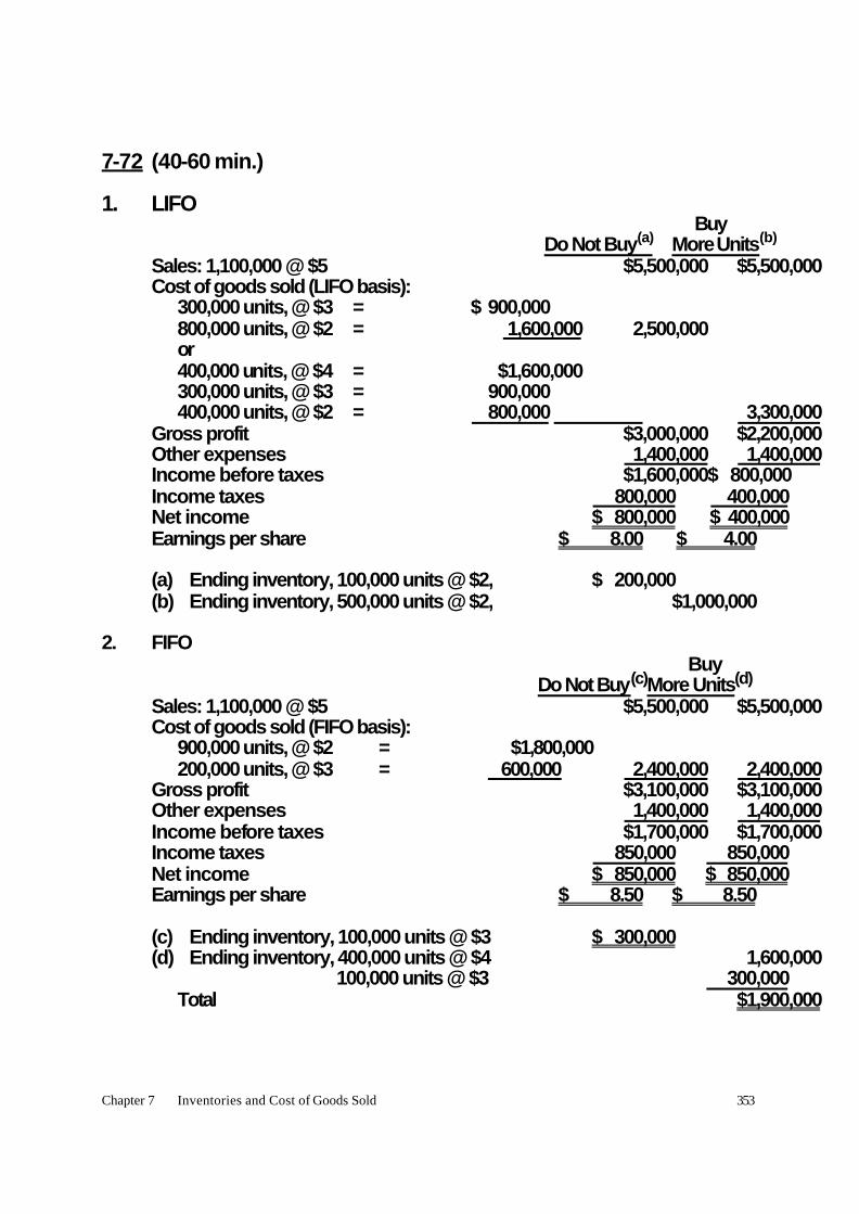
7-72 (40-60 min.) 1. LIFO Buy Do Not Buy(a) More Units(b)

Sales: 1,100,000 @ $5 $5,500,000 $5,500,000 Cost of goods sold (LIFO basis): 300,000 units, @ $3 = $ 900,000 800,000 units, @ $2 = 1,600,000 2,500,000 or 400,000 units, @ $4 = $1,600,000 300,000 units, @ $3 = 900,000 400,000 units, @ $2 = 800,000 3,300,000 Gross profit $3,000,000 $2,200,000 Other expenses 1,400,000 1,400,000 Income before taxes $1,600,000$ 800,000 Income taxes 800,000 400,000 Net income $ 800,000 $ 400,000 Earnings per share $ 8.00 $ 4.00

(a) Ending inventory, 100,000 units @ $2, $ 200,000 (b) Ending inventory, 500,000 units @ $2, $1,000,000 2. FIFO Buy Do Not Buy(c)More Units(d)

Sales: 1,100,000 @ $5 $5,500,000 $5,500,000 Cost of goods sold (FIFO basis): 900,000 units, @ $2 = $1,800,000 200,000 units, @ $3 = 600,000 2,400,000 2,400,000 Gross profit $3,100,000 $3,100,000 Other expenses 1,400,000 1,400,000 Income before taxes $1,700,000 $1,700,000 Income taxes 850,000 850,000 Net income $ 850,000 $ 850,000 Earnings per share $ 8.50 $ 8.50

(c) Ending inventory, 100,000 units @ $3 $ 300,000 (d) Ending inventory, 400,000 units @ $4 1,600,000 100,000 units @ $3 300,000 Total $1,900,000

354

7-72 (continued) 3. Consider this question from a strict financial management

standpoint – ignoring earnings per share. When prices are rising, it may be advantageous – subject to prudent restraint as to maximum and minimum inventory levels – to buy unusually heavy amounts of inventory at year-end, particularly if income tax rates are likely to fall. Under LIFO, the current year tax savings would be a handsome $400,000. This is at least a deferral of the tax effect. The effects on later years' taxes will depend on inventory levels, prices, and tax rates.

Tax savings can be generated because LIFO permits

management to influence immediate net income by its purchasing decisions. In contrast, FIFO results would be unaffected by this decision.

However, if management buys the 400,000 units and uses

LIFO, the first year earnings per share would be only $4.00. Note too that LIFO will show less earnings per share than FIFO ($8.00 as compared to $8.50), even if the 400,000 units are not bought. Such results may cause management to reject LIFO. Earnings per share (EPS) is a critical number, and many managements are reluctant to adopt accounting policies that hurt EPS.

The shame of the matter is that the same business events can

dramatically affect measures of performance, depending on whether LIFO or FIFO is adopted ($4.00 versus $8.50). Although, the smart decision would be to adopt LIFO and buy the 400,000 units, this decision produces the worst earnings record!

4a. The income statement for year two would show the same net

income and earnings per share whether additional inventory is purchased or not, because prices do not change.

356

7-72 (continued)

LIFO FIFO In year 2 Do not Buy Buy Do not Buy Buy Sales $5,500,000 $5,500,000 $5,500,000 $5,500,000 Cost of goods sold 4,400,000(a) 4,400,000(b) 4,300,000(c) 4,300,000(d) Gross profit $1,100,000 $1,100,000 $1,200,000 $1,200,000 Other expenses 800,000 800,000 800,000 800,000 Income before taxes $ 300,000 $ 300,000 $ 400,000 $ 400,000 Income taxes 120,000 120,000 160,000 160,000 Net income $ 180,000 $ 180,000 $ 240,000 $ 240,000 Earnings per share $ 1.80 $ 1.80 $ 2.40 $ 2.40 Year 2 Cost of Goods Sold Calculations

(a) (b) (c) (d) Beginning inventory,

see parts (1) and (2)

$ 200,000

$1,000,000

$ 300,000

$1,900,000 Purchases: 1,700,000 units @ $4 6,800,000 6,800,000 1,300,000 units @ $4 5,200,000 5,200,000 Available for sale $7,000,000 $6,200,000 $7,100,000 $7,100,000 Ending inventory: 100,000 units @ $2 = $ 200,000 600,000 units @ $4 = 2,400,000 2,600,000 500,000 units @ $2 = 1,000,000 200,000 units @ $4 = 800,000 1,800,000 700,000 units @ $4 =

2,800,000 2,800,000

Cost of goods sold $4,400,000 $4,400,000 $4,300,000 $4,300,000 4b. FIFO shows $100,000 higher income before taxes ($60,000

after taxes) because 100,000 units of old, lower-cost inventory is in Cost of Goods Sold:

LIFO FIFO 1,000,000 units @ $4 = $4,000,000 100,000 units @ $3 = 300,000 1,100,000 units @ $4 = $4,400,000 $4,300,000


7-72 (continued) 4c. The ending LIFO inventory is $800,000 higher in column (a)

because the 400,000 more units in ending inventory are priced at $4 a unit when the inventory is not replenished at the end of year one. In column (b), the 400,000 units purchased @ $4 near the end of the first year were charged immediately to Cost of Goods Sold, leaving 400,000 more of the ending inventory units at the old unit cost of $2. Under the LIFO assumption, this inventory is regarded as untouched in the second year, so the old $2 unit cost applies to the ending inventory of the second year.

4d. Alternatives a b c d

Income tax for the two years $920,000 $520,000 $1,010,000 $1,010,000

Unless the LIFO layers are depleted, the adoption of LIFO will result in permanent postponement of income taxes. However, if the layers are invaded, these low-cost layers will cause higher tax payments in later years than under FIFO.

4e. As far as the financial decision is concerned, the computations

in part (4) substantiate the conclusions in part (3). As far as EPS is concerned, note that all EPS numbers decline in the second year.

358

7-73 (30 min.) This problem highlights the fact that LIFO theory of matching current costs against current revenues breaks down when the so-called LIFO-base inventory is invaded. Then the costs matched against current revenue are a conglomeration of old (often ancient) costs and current costs. If prices have been rising for a long time, the income tax liability can be unusually severe: Requirement (1) Requirement (2) Sales, 500,000 units @ $3.00 $1,500,000 $1,500,000 Cost of goods sold: 340,000 @ $2.00 = $680,000 500,000 @ $2.00 1,000,000 30,000 @ 1.20 = 36,000 50,000 @ 1.10 = 55,000 80,000 @ 1.00 = 80,000 851,000 Gross profit 649,000 500,000 Operating expenses 500,000 500,000 Net income before taxes 149,000 − Income taxes @ 60% 89,400 − Net income $ 59,600 $ −


7-74 (15-20 min.)

1. Figures are in millions of dollars.

Lower of LIFO LIFO Cost Cost or Market 2003 2004 2003 2004

Sales 20 8 20 8 Cost of goods sold 14 13 14 8 Write-down of ending inventory – – 5 – Total costs charged against sales 14 13 19 8 Gross margins without write-down 6 (5) Gross margin after write-down 1* 0

* Accountants use various formats for presenting the effects of write-

downs. Some deduct the write-down as a special loss immediately after gross margin rather than having it affect gross margin. Thus, under LIFO some would calculate the standard LIFO gross margin and then adjust it.

Gross margin 5 Write-down 4 Gross margin less inventory write-down 1

The total gross margin for the two years combined is the same for LIFO and lower-of-LIFO-or-market. The lower-of-cost-or-market method is labeled as more conservative because it shows gloomier results earlier in a series of periods.

2. If replacement cost were $9 million on January 31, 2004, no restoration of the December write-down would be permitted. In brief, the $8 million December 31 valuation became the "new cost" of the inventory. Inasmuch as only write-downs below cost are allowed in historical cost accounting for inventories, no subsequent write-ups are allowed.

360

7-75 (15-20 min.)

1. The change in the LIFO reserve is the annual effect on cost of goods sold; in this instance $86.094 million – $83.829 million = $2.265 million. Because the LIFO reserve rose, the use of LIFO in this year decreased pretax income by $2.265 million. Therefore, using FIFO, pretax income would have been $359.495 million + $2.265 million = $361.760 million.

2. LIFO = .34 x $359,495,000 = 122,228,300 FIFO = .34 x $361,760,000 = 122,998,400 Difference = 770,100 Difference = .34 x 2,265,000 = 770,100

3. Yes. LIFO use reduced taxes in the current year by $770,100. Historically the cumulative effect can be estimated by multiplying the tax rate times the LIFO Reserve. .34 x $86.094 million = $29.272 million. Think of this as an interest free loan from the government.


7-76 (15-20 min.)

1. Increasing. FIFO reports the most recent costs on the balance sheet; LIFO reports older costs. Because FIFO amounts exceed LIFO amounts, the most recent costs must be higher than older costs. Therefore, costs have been increasing.

2. Amounts in millions:

(a) LIFO

(b) FIFO

Sales revenue $700.0 $700.0 Cost of goods sold 546.9 632.6* Gross profit $153.1 $ 67.4

* $546.9 + $85.7 = $632.6

Gross profit is higher under LIFO. Old LIFO layers are charged as cost of goods sold. Because prices have been increasing, the cost of old LIFO layers is less than more recent costs. Therefore, LIFO cost of goods sold is less than FIFO cost of goods sold, resulting in more gross profit under LIFO when existing inventories are completely liquidated.

362

7-77 (10-15 min.)

O is used for overstated, U for understated, and N for not affected. All amounts are $10 million unless otherwise indicated. 1. Effects of Fiscal Year 2002 2001

Beginning inventory O N Ending inventory N O Cost of sales O U Gross profit U O Income before taxes U O Taxes on income U by $4mil* O by $4 mil* Net income U by $6 mil** O by $6 mil** *. 40 x $10 million = $4 million ** (1 – .40) x $10 million = $6 million

2. Retained earnings would be overstated by $6 million at the end of fiscal 2001. However, the error would be offset in the next year assuming no change in the 40% rate of income tax. Therefore, retained earnings would be correct at the end of fiscal 2002.


7-78 (20-30 min.)

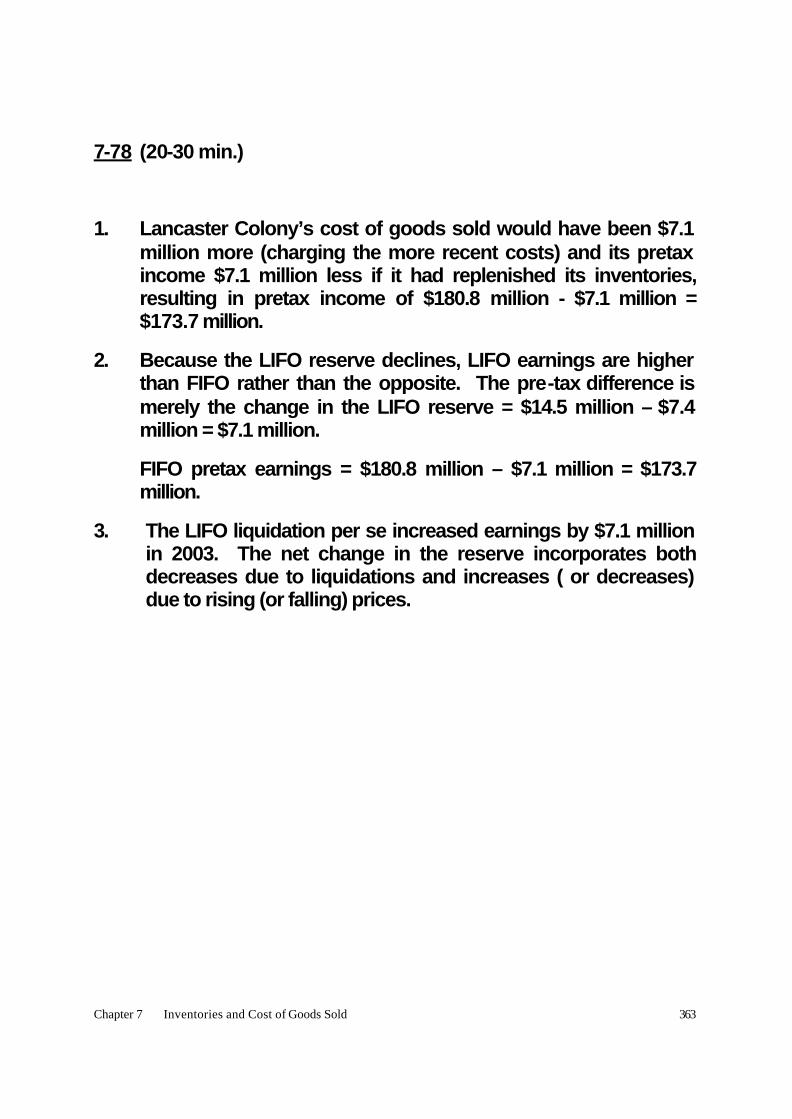
1. Lancaster Colony’s cost of goods sold would have been $7.1 million more (charging the more recent costs) and its pretax income $7.1 million less if it had replenished its inventories, resulting in pretax income of $180.8 million - $7.1 million = $173.7 million.

2. Because the LIFO reserve declines, LIFO earnings are higher than FIFO rather than the opposite. The pre-tax difference is merely the change in the LIFO reserve = $14.5 million – $7.4 million = $7.1 million.

FIFO pretax earnings = $180.8 million – $7.1 million = $173.7 million.

3. The LIFO liquidation per se increased earnings by $7.1 million in 2003. The net change in the reserve incorporates both decreases due to liquidations and increases ( or decreases) due to rising (or falling) prices.

364

7-79 (10-15 min.) 1. Cost of goods sold:

With the purchase, $380 x 8,000 $3,040,000 Without the purchase, $250 x 8,000 2,000,000 Difference $1,040,000 Income tax savings, .40 x $1,040,000 $ 416,000

2. This is an actual case. The only change is that the original

numbers were $300 and $160 rather than the $380 and $250 used here. The Tax Court held that raw materials may be entered as inventory only if they have been acquired for the purpose of sale in the ordinary course of business or for the purpose of being physically incorporated into merchandise intended for sale. Therefore, the taxpayer's cost of goods sold should have included the cost of the lower-priced inventory instead of the higher-priced year-end purchase.


7-80 (15-20 min.)

Gross Profit Percentage Inventory Turnover Penney 03 $9,774÷$32,347 = .302 $22,573÷$4,938 = 4.57 00 $9,136÷$32,510 = .281 $23,374÷$6,004 = 3.89 95 $6,410÷$20,380 = .315 $13,970÷$3,711 = 3.76 Kmart 03 $4,504÷$30,762 = .146 $26,258÷$5,311 = 4.94 00 $7,823÷$35,925 = .218 $28,102÷$6,819 = 4.12 95 $8,033÷$34,025 = .236 $25,992÷$7,317 = 3.55

J.C. Penney has a consistently higher gross profit percentage than Kmart. J.C. Penney generated higher inventory turnover than Kmart in 1995 but not in 2000 or 2003. For J.C. Penney, gross profit percentage fell while inventory turnover improved in 2000 compared to 1995, but both ratios improved significantly by 2003. Kmart consistently improved its inventory turnover but had a significant decline in gross profit percentage. Penney's higher gross margin percentage no doubt reflects its chosen market niche which places more emphasis on style and fashion and less on price. It is strange, however, that given Kmart's low price strategy that Kmart's turnover was lower than J.C. Penney's in 1995. In 2000 and 2003 Kmart’s inventory turnover exceeded that of J.C. Penney, as one would normally expect. It is instructive to relate these values to those for a company like The Gap. The Gap’s 2002 gross profit percentage was about 34% and inventory turnover was about 5.

366

7-81 (15 min.) Amounts are in millions. 2003: Gross profit = KRW 59,569 − KRW 36,952 = KRW 22,617 Gross profit percentage = KRW 22,617 ÷ KRW 59,569 = 38.0% Inventory turnover = KRW 36,952 ÷KRW 3,954 = 9.3 2002: Gross profit = KRW 46,444 − KRW 32,657 = KRW 13,787 Gross profit percentage = KRW 13,787 ÷ KRW 46,444 = 29.7% Inventory turnover = KRW 32,657 ÷ KRW 3,611 = 9.0 The gross profit percentage increased from 29.7% to 38.0%, and the inventory turnover increased from 9.0 to 9.3. Both of these are good news to Samsung. The large increase in gross profit percentage is especially significant.


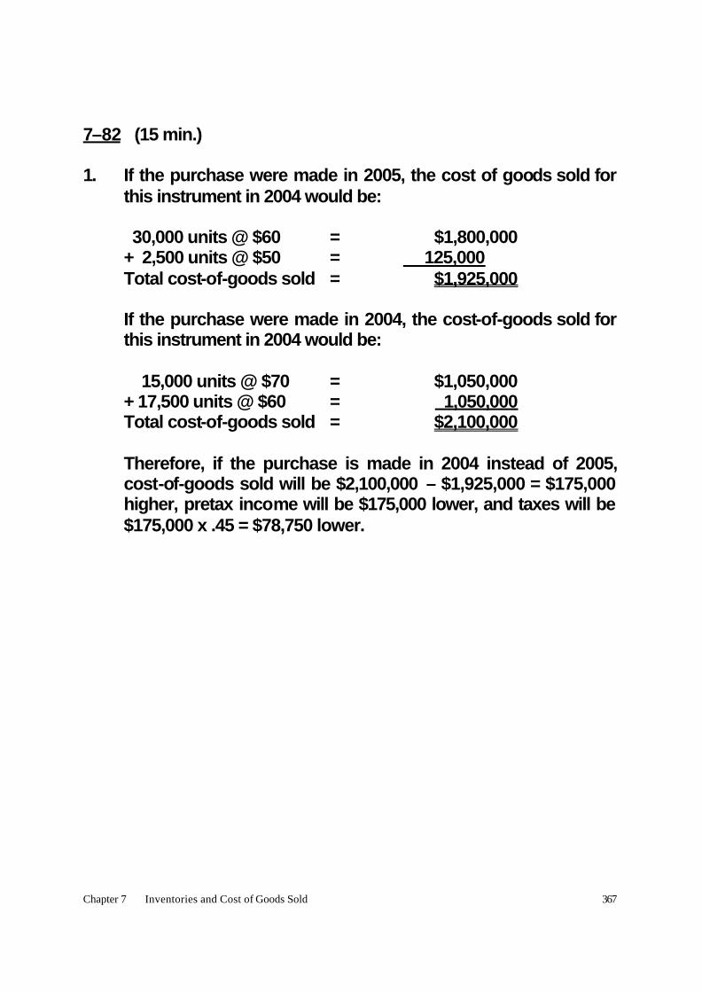
7–82 (15 min.) 1. If the purchase were made in 2005, the cost of goods sold for

this instrument in 2004 would be: 30,000 units @ $60 = $1,800,000 + 2,500 units @ $50 = 125,000 Total cost-of-goods sold = $1,925,000 If the purchase were made in 2004, the cost-of-goods sold for

this instrument in 2004 would be: 15,000 units @ $70 = $1,050,000 + 17,500 units @ $60 = 1,050,000 Total cost-of-goods sold = $2,100,000 Therefore, if the purchase is made in 2004 instead of 2005,

cost-of-goods sold will be $2,100,000 – $1,925,000 = $175,000 higher, pretax income will be $175,000 lower, and taxes will be $175,000 x .45 = $78,750 lower.

368

7–82 (continued) 2. The LIFO inventory method allows managers and accountants

to manipulate income by purchases made near the end of the year. A manager in Yokohama may want to maximize net income, even if it results in higher taxes for the company. Perhaps the manager has a bonus that depends on the company’s net income. Such a manager might prefer the purchase to be delayed until 2005.

It is not clear whether a 2004 or 2005 purchase (if either) is best

for Yokohama. The savings in taxes by purchasing in 2004, which will be offset by higher taxes in subsequent years, is beneficial because it defers the taxes, giving Yokohama the $78,750 to use in the meantime. However, maybe there is a debt covenant that may be violated if the extra $175,000 of pretax income (and, therefore, an extra $96,250 net income) is not generated in 2004. Or maybe the current ratio will drop below an acceptable level if purchase is delayed to 2005.

Although there is not enough information to decide what is the

best decision for Yokohama, it is clear that manipulation of income is possible under LIFO. This is likely to create ethical dilemmas for managers whose performance evaluations (and possibly personal wealth) may be linked to financial results or who envision reported earnings affecting share price or debt covenants.


7-83 (15 min.) 1.

Inventory Balance 135,000 590,000 630,000 Balance X

Let X be the ending inventory balance:

X = Beginning balance + Purchases − Cost of goods sold X = $135,000 + $630,000 − $590,000 = $175,000

2. Inventory shrinkage = $175,000 − $140,000 = $35,000

Inventory shrinkage expense 35,000 Inventory 35,000 Cost of goods sold = $590,000 + $35,000 = $625,000

3. Inventory shrinkage as a percent of sales is $35,000 ÷ $700,000 = 5.0%. This is high. Lola should look for ways that inventory might be stolen, either by employees or by others. She also may want to examine the new perpetual inventory system to make sure that all costs of goods sold are being recorded.

370

7-84 (15-20 min.)

1. An understatement of ending inventories overstates cost of goods sold and understates taxable income by $500,000. Taxes evaded would be .40 x $500,000 = $200,000.

2. This news story provides a good illustration of why a basic knowledge of accounting is helpful in understanding the business press. The news story is incomplete or misleading in one important respect. The business owner's understated ending inventory becomes the understated beginning inventory of the next year. If no other manipulations occur, the owner will understate cost of goods sold during the next year, overstate taxable income, and pay an extra $200,000 in income taxes. Thus, the owner will have postponed paying income taxes for one year, paying no interest on the money "borrowed" from the government.

To continue to evade the $200,000 of income taxes of year one, the ending inventory of the second year must be understated by $500,000 again. However, if only the $500,000 understatement persists year after year, the owner is enjoying a perpetual loan of $200,000 (based on a 40% tax rate) from the government. Data follow (in dollars):


7-84 (continued) Honest Reporting Dishonest Reporting

First Year Second Year First Year Second Year

Beginning inventory 3,000,000 2,500,000 3,000,000 2,000,000 Purchases 10,000,000 10,000,000 10,000,000 10,000,000 Available for sale 13,000,000 12,500,000 13,000,000 12,000,000 Ending inventory 2,500,000 2,500,000 2,000,000 2,000,000 Cost of goods sold 10,500,000 10,000,000 11,000,000 10,000,000 Income tax savings @ 40% 4,200,000 4,000,000 4,400,000 4,000,000 Income tax savings for

two years together 8,200,000 8,400,000

Some students may incorrectly reason that understating inventory each year has a cumulative effect. You may wish to emphasize that the second year has the same cost of goods sold in each column, because in the "dishonest" case both beginning and ending inventory are understated by the same amount. To evade an additional $200,000 of income taxes in the second year, the ending inventory must be understated by $1,000,000 (not $500,000) in the second year.

372

7-85 (15-20 min.) 1. Raw material used = 1,500 shirts @ $3 = $4,500

Wages paid = 1 month = 1,600

Depreciation = 1,500 units @ [$5,000 ÷ 10,000 = .50] = 750

Studio rent = 500

Total production costs $7,350

Cost per unit produced = $7,350 ÷ 1,500 =$ 4.90

Cost of goods sold = 1,200 x $4.90 = $5,880

Ending inventory:

Raw material available 500 shirts @ $3 = $1,500

Finished goods 1,500 – 1,200 =

300 shirts @ $4.90 = 1,470

Total inventory $2,970 2. SAM’S T-SHIRTS Income Statement for January

Revenue 1,200 shirts @ $9 $10,800 Cost of goods sold 5,880 Income before tax 4,920 Tax expense 1,476 Net Income $ 3,444


7-86 (60 min. or more) The purpose of this exercise is to develop an understanding of inventory methods and to be able to explain an inventory method to others. An individual student could compute the operating income using all three methods, but using a team has two main advantages: 1. Each student can become thoroughly familiar with one

inventory method; students do not need to spend time making calculations for all methods.

2. Explaining the computations involved with one inventory method requires a deeper understanding than merely carrying out the calculations.

A good starting point is to examine the 1987 and 1988 T-

accounts for inventory under LIFO and FIFO (amounts are in thousands): 1987:

Inventory (FIFO) Inventory (LIFO)

Beg. Bal. 151,918 CGS 533,355* Beg. Bal. 140,918 CGS 533,555 Purchases 562,125 Purchases 562,125 End. Bal. 180,688 End. Bal. 169,488

* FIFO CGS is $200,000 less than LIFO CGS because FIFO inventory increased $200,000 more than did LIFO inventory in 1997.

1988:

Inventory (FIFO) Inventory (LIFO)

Beg. Bal. 180,688 CGS 559,883 Beg. Bal. 169,488 CGS 560,233 Purchases 560,233 Purchases 560,233 End. Bal. 181,088 End. Bal. 169,488 The operating income statements for each inventory method are:

374

7-86 (continued) FIFO: Sales $1,015,198 Cost of goods sold (using FIFO) 559,833 Other operating expenses 417,283 Operating income $ 38,082 LIFO: Sales $1,015,198 Cost of goods sold (using LIFO) 560,233 Other operating expenses 417,283 Operating income $ 37,682 Specific identification:

There is not enough information to compute a definitive profit under specific identification. Probably the physical flow of merchandise is closest to FIFO, so operating income would be close to $46,716. However, to the extent that a strict FIFO flow is not maintained, operating income would fall short of $38,082. Why? Because some of the recent purchases, which cost 5% more than earlier purchases, would be sold and the earlier purchases would remain in inventory, boosting cost of goods sold and decreasing inventory from the FIFO levels.

7–87 (45-60 min.) Each solution will be unique and will change each year. The

purpose of this problem is to recognize different inventory methods and their relationship to gross profit percentage and inventory turnover.


7–88 (35-45 min.) Amounts are in thousands. Inventory Calculation 1. Inventory Beginning + Purchases – Sales = Ending 263,174 263,174 + Purchases – 1,348,742 = 342,944

1,428,512 1,348,742* Purchases = 342,944 + 1,348,742 – 263,174 342,944 Purchases = $1,428,512 *$1,685,928 x .8 = $1,348,742 2. Inventory turnover = Cost of sales ÷ average inventory Inventory turnover = $1,348,742 ÷ ($342,944 + $263,174) ÷

2 = $1,348,742 ÷ $303,059 = 4.45

3. Error! $4,075,522

$1,348,742 $4,075,522 − = .67 2003

1 $3,288,908 $3,288,908

009,080,$− = .67 2002

980,648,2$

228,890$ 980,648,2$ − = .66 2001

The gross margin percentage has risen very slightly over the

three years. Gross margins for Starbucks are high. This is because of the

industry and Starbucks’ strategy. Starbucks charges a premium price for its coffee and other drinks.

376

7-89 (30-60 min.)

NOTE TO INSTRUCTOR. This solution is based on the web site as it was in late 2004. Be sure to examine the current web site before assigning this problem, as the information there may have changed. 1. In 2003 Teva represented 60.1% of Deckers’ sales. This percentage has dropped steadily in the last 5 years from 72.9% in 1999, even though total sales of Tevas have increased. 2. Inventories are reported at the lower of FIFO cost or market. The costs of inventories are probably not increasing fast enough to give LIFO a large tax advantage. Using LCM is important to a company such as Deckers because shoes can become out-of-style and therefore have market values below cost. In 2003 Deckers has a write-down of inventory of $882,000. 3. In 2003 the gross profit was $51,345,000, up from $41,530,000 in 2002. The gross profit percentage increased from 41.9% to 42.4% over the same year. Management indicated that “The increase in gross margin was due to several factors, including an above average gross margin at the newly acquired Internet and catalog retailing business, the favorable impact of the strong Euro, and lower production overhead costs per pair, partially offset by an increase in close-out sales.”

CHAPTER 7 perpetual system and conceptually … 7 Inventories and Cost of Goods Sold 303 7-30 There...

Documents

Transcript of CHAPTER 7 perpetual system and conceptually … 7 Inventories and Cost of Goods Sold 303 7-30 There...