Chapter 7.

Inequality and social mobility in the Era of the Industrial Revolution

Gregory Clark and Neil Cummins

2

1. Introduction

This chapter examines the effects of the Industrial Revolution on

social mobility rates and inequality, as England experienced the onset of

modern economic growth. It has previously been impossible to measure

social mobility rates before the end of the Industrial Revolution, because

population censuses showing family relationships only become available

in 1851. However, we show how, using information on surname

distributions, intergenerational social mobility rates back to 1700 can be

calculated. These show that social mobility rates have always been low in

England and were surprisingly unaffected by the Industrial Revolution.

Modern growth did not speed up the process of intergenerational mobility.

In addition we show that the Industrial Revolution era was probably one of

declining inequality in England. While we do not have information on the

individual distribution of income and wealth, we can show that the share of

wages in national income increased in Industrial Revolution England.

Since wages are distributed in all societies much more equally than

income from property, this would have been a force for greater income

equality within industrial society.

2. Social Mobility

Was the Industrial Revolution associated with a period of enhanced

social mobility? And how did social mobility rates then compare with

those of modern Britain? We might expect that the Industrial Revolution

would have disrupted the old social classes and created a period of

enhanced mobility, compared to what came before, both upwards and

downwards. Change and disruption would favour mobility. Stasis and

continuity would embed immobility.

Change there certainly was in Britain after 1760. There was the

creation of new industries and new occupations. The old landed

aristocracy began to be replaced by a new industrial, commercial and

technical class, affording opportunities for mobility to those who had

heretofore lived as agricultural labourers in semi-feudal dependence. At

3

the same time large numbers of relatively prosperous handicraft producers

were displaced by the arrival of factory production. The hand-loom

weavers, often owners of their looms and cottages, were displaced by low

paid factory weavers. There was a large scale movement of the

population out of agriculture and the countryside and into growing urban

centers. The previously poor and economically underdeveloped north of

England, together with Scotland, rose to become centers of wealth and

power. There was an influx of poor immigrants from Ireland into the

British industrial cities.

However, contemporaries had conflicted views of social mobility in

Industrializing England. The so-called Condition-of-England novels of the

Victorian Era, such as Benjamin Disraeli’s Sybil (1845), Charles Dickens’

Hard Times (1854), and Elizabeth Gaskell’s North and South (1855), for

example, offer clashing perspectives on social mobility within the same

works. These works feature self-made industrialists, men made upwardly

mobile by the new economic possibilities. But they also feature a new

class of industrial workers seemingly locked in place, facing a growing

divide between themselves and the industrial aristocracy. What was the

aggregate effect of these changes on social mobility? Did mobility

increase as a result of the Industrial Revolution? And how do mobility

rates in 1700-1870 compare with those of today?

The standard method of estimating intergenerational social mobility in

England in the nineteenth century has been to compare the occupations of

grooms versus their fathers in marriage registers; those occupations are

systematically recorded only from 1837. Studies of these registers

suggest that Industrial Revolution England remained a socially immobile

society. Miles, for example, studying thousands of register entries for

England, concluded that fewer than 40% of grooms in mid-nineteenth

century England had an occupational class different from that of their

father. England was “in terms of its inhabitants’ relative life chances, a

profoundly unequal society” (Miles 1999:177).

Table 7.1 about here%

4

Table 7.2 about here%

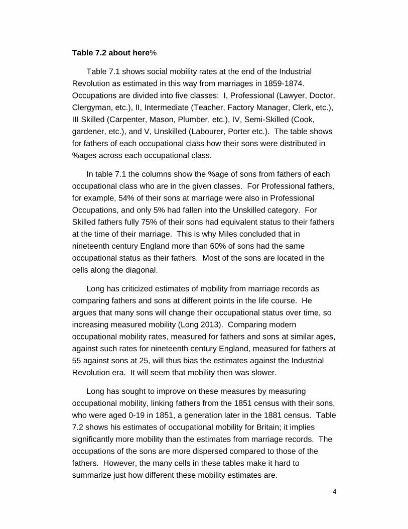
Table 7.1 shows social mobility rates at the end of the Industrial

Revolution as estimated in this way from marriages in 1859-1874.

Occupations are divided into five classes: I, Professional (Lawyer, Doctor,

Clergyman, etc.), II, Intermediate (Teacher, Factory Manager, Clerk, etc.),

III Skilled (Carpenter, Mason, Plumber, etc.), IV, Semi-Skilled (Cook,

gardener, etc.), and V, Unskilled (Labourer, Porter etc.). The table shows

for fathers of each occupational class how their sons were distributed in

%ages across each occupational class.

In table 7.1 the columns show the %age of sons from fathers of each

occupational class who are in the given classes. For Professional fathers,

for example, 54% of their sons at marriage were also in Professional

Occupations, and only 5% had fallen into the Unskilled category. For

Skilled fathers fully 75% of their sons had equivalent status to their fathers

at the time of their marriage. This is why Miles concluded that in

nineteenth century England more than 60% of sons had the same

occupational status as their fathers. Most of the sons are located in the

cells along the diagonal.

Long has criticized estimates of mobility from marriage records as

comparing fathers and sons at different points in the life course. He

argues that many sons will change their occupational status over time, so

increasing measured mobility (Long 2013). Comparing modern

occupational mobility rates, measured for fathers and sons at similar ages,

against such rates for nineteenth century England, measured for fathers at

55 against sons at 25, will thus bias the estimates against the Industrial

Revolution era. It will seem that mobility then was slower.

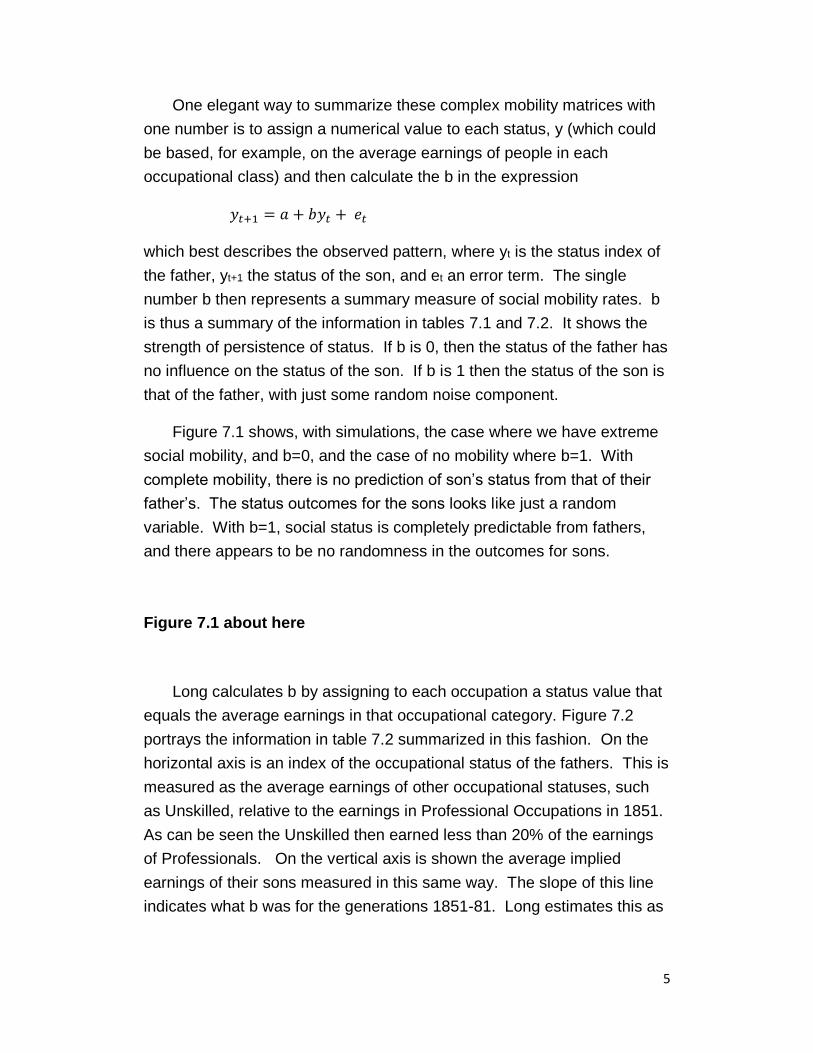
Long has sought to improve on these measures by measuring

occupational mobility, linking fathers from the 1851 census with their sons,

who were aged 0-19 in 1851, a generation later in the 1881 census. Table

7.2 shows his estimates of occupational mobility for Britain; it implies

significantly more mobility than the estimates from marriage records. The

occupations of the sons are more dispersed compared to those of the

fathers. However, the many cells in these tables make it hard to

summarize just how different these mobility estimates are.

5

One elegant way to summarize these complex mobility matrices with

one number is to assign a numerical value to each status, y (which could

be based, for example, on the average earnings of people in each

occupational class) and then calculate the b in the expression

𝑦𝑡+1 = 𝑎 + 𝑏𝑦𝑡 + 𝑒𝑡

which best describes the observed pattern, where yt is the status index of

the father, yt+1 the status of the son, and et an error term. The single

number b then represents a summary measure of social mobility rates. b

is thus a summary of the information in tables 7.1 and 7.2. It shows the

strength of persistence of status. If b is 0, then the status of the father has

no influence on the status of the son. If b is 1 then the status of the son is

that of the father, with just some random noise component.

Figure 7.1 shows, with simulations, the case where we have extreme

social mobility, and b=0, and the case of no mobility where b=1. With

complete mobility, there is no prediction of son’s status from that of their

father’s. The status outcomes for the sons looks like just a random

variable. With b=1, social status is completely predictable from fathers,

and there appears to be no randomness in the outcomes for sons.

Figure 7.1 about here

Long calculates b by assigning to each occupation a status value that

equals the average earnings in that occupational category. Figure 7.2

portrays the information in table 7.2 summarized in this fashion. On the

horizontal axis is an index of the occupational status of the fathers. This is

measured as the average earnings of other occupational statuses, such

as Unskilled, relative to the earnings in Professional Occupations in 1851.

As can be seen the Unskilled then earned less than 20% of the earnings

of Professionals. On the vertical axis is shown the average implied

earnings of their sons measured in this same way. The slope of this line

indicates what b was for the generations 1851-81. Long estimates this as

6

b = 0.36. The figure also shows the data for the mobility estimates from

marriage certificates. Here the implied b is much higher at 0.64.

Figure 7.2 about here

Table 7.3 about here

The b estimated by Long implies that Britain, at the end of the

Industrial Revolution, had a relatively high degree of social mobility. One

way to see this is to consider that when we measure social mobility in this

way, b2 is the share of variation in social status that is predictable at birth.

As can be seen in figure 7.1, when b=1, all the variation among sons is

predictable at birth, when b=0, none of it is predictable. Long’s b of 0.36

for 1851-1881 implies that by the end of the Industrial Revolution era, only

13% of occupational status variation came from inheritance. In contrast

the marriage register data implies that 41% of the variation in status is

explained by inheritance.

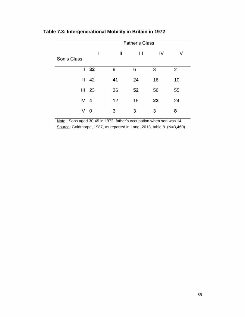
How does this Victorian occupational mobility compare to modern

social mobility rates in Britain? Table 7.3 shows the equivalent

occupational mobility table for modern Britain in 1972, based on the

occupations of sons aged 30-49 in that year compared to their fathers’

occupations when the sons were 14. As before each column shows the

distribution, in %ages, of the sons of fathers of a given occupational class.

Again it is hard to see in this complex set of cells whether occupational

mobility was much greater than in Long’s equivalent table for 1851-81.

But we can also portray this data in figure 7.2 as a curve relating the

average status of fathers to that of sons. Because occupational wage

differentials are more compressed in modern England, the social class of

fathers is more compressed. But the slope of the line connecting fathers

and sons seems similar to that for 1851-81. And indeed Long estimates,

from Goldthorpe’s data, that the b for 1972 is 0.32. This implies that

modern Britain had modestly greater occupational mobility rates than late

7

Industrial Revolution Britain. But these studies suggest that both are

actually mobile societies, with lots of significant transitions in status

between fathers and sons.

However, there seems little prospect of extending Long’s type of

analysis of occupational mobility any earlier than the census of 1841.

Before that, linkage of the status of specific fathers and sons on a

systematic basis on a large scale has not yet been achieved.

Some authors have sought to measure mobility rates by looking at

linkages between the occupations of fathers and sons in partial sources.

Sanderson, for example, used the records of the Charity School in

Lancaster in 1770-1816, which gives the occupation of the fathers of the

boys attending as well as the occupational destination of the boys, to

measure upward mobility rates in the early Industrial Revolution. He finds

that of 38 sons whose fathers were labourers, only 2 ended up in similarly

unskilled occupations (Sanderson 1972:99). There is substantial upward

mobility. But this is a selective group of sons of labourers, those who

ended up at school. Naturally they display substantial upward mobility.

They cannot tell us about general mobility rates.

A more promising source is that employed by Humphries: 617 working

class autobiographies of the years up to 1878, which portray the careers

of members of the working class in this era (Humphries 2010). This

dataset also offers measures of the linkage of parent and child

occupational status earlier in the Industrial Revolution. Humphries’ data is

not organized in a way so as directly to measure intergenerational social

mobility. But it does suggest that these working class autobiographers

overwhelmingly had fathers with lower class origins, all through the

Industrial Revolution years. This is what explains the frequency of child

labour by the writers, the lack of formal education, and the accounts of

childhood hunger so frequent in these autobiographies. If Long’s data in

table 7.3 is correct, then about 20% of working class males would have

middle or upper class fathers in Industrial Revolution England. So

Humphries’ autobiographers seemingly show much less social mobility

than would be expected from the Long study. Social mobility may indeed

have been low in Industrial Revolution England.

8

However, even though Humphries’ shows that the working class

biographies are representative of the occupational structure of Industrial

Revolution England, there will be questions about whether the

autobiographers are representative in terms of social mobility. Could it be

that in the age of Samuel Smiles’ Self Help (1859), those who survived

adversity, or even triumphed over adversity, would be more inclined to

record their histories than those who, despite the privileges of birth, fell

into the working class through illness, bad luck, alcoholism, sloth, mental

incapacity, or bankruptcy?

There is another way, however, of measuring social mobility, which

exploits the fact that surnames are inherited, which can be applied to

England all the way back to 1700. If social mobility is rapid, then

surnames which in the current period have a high or low average social

status, should quickly regress towards mean status. Surnames are

inherited by sons, and if sons of fathers of high and low status are

regressing quickly towards average status, so should the surnames they

bear move quickly to average status. The speed of the loss of information

content about status in surnames can be translated into an implied rate of

social mobility, the b above.

To carry out this calculation of b from surnames all we need to

observe is the share of a surname in the general population in each

generation, and their share in an elite group within the population (Clark

and Cummins, 2012). From this we can calculate for each surname its

relative representation among the elite: its share among the elite divided

by its share in the general population. For common surnames, such as

Williams, Green or Clark, their relative representation will always be close

to 1 in England by 1700. They have the same frequency in elites as in the

general population, and people at all statuses in the society hold the

surname. However, some rare surnames, such as Pepys, Boscawen, or

Champion de Crespigny will be found disproportionately among elites in

1700. Their relative share in elites can be 10 or 20 times as great as in

the general population. The decline of that relative representation in each

generation towards 1 shows the rate of social mobility. The slower is the

rate of decline, the less is social mobility, and the lower the implied value

of b.

9

Figure 7.3 illustrates this process. Suppose in generation 0 a set of

surnames is 10 times as common in the top 5% of the status distribution

as in the population as a whole. Their implied decline in relative

representation across each generation is shown for different values of b:

0.25, 0.5, and 0.75. As can be seen if b is 0.25, which would be similar to

some values estimated for occupational status persistence in England

both in the nineteenth and twentieth centuries, then within 3 generations

the high status surnames would have declined to average status. While if

b is 0.75, then even after 5 generations these surnames would still be

overrepresented among elites.1

Figure 7.3 about here

One elite group we observe all the way from 1700 to 1858, for

example, are the people whose estates were probated in the highest

probate court in the land, the Prerogatory Court of the Archbishop of

Canterbury (PCC). This was the court where the elites of English society,

by wealth and occupation, had their wills proved at death. The share of

men dying in England with wills proved in this court was fairly stable over

these years, averaging 5.3% of all adult male deaths. Thus we can take

those testators proved in this court as representing the top 5.3% of wealth

holding in English society.2 In the north of the country the estates of high

status individuals might instead be probated in the Prerogatory Court of

the Archbishop of York. But in 1809 when we can first observe the values

of the estates proved in each court, the estates proved in the York court

were significantly less substantial on average than those of the Canterbury

Court.

By 1700 about a quarter of the wills probated in the PCC were from

women, typically from women who were widows or spinsters. So while

1 The assumptions required for this calculation are just that status is normally distributed with the same variance in the general population and the elite surname subgroup. 2

10

this measure will mainly show the inheritance of wealth by men, the

inclusion of these women means that it is a bit broader, and is about the

general inheritance of wealth within families.

Using the PCC we can form sets of rare surnames that showed up in

these probates 1680-1709, 1710-39, 1740-69, 1770-1799, corresponding

to generations of 30 years.3 We can tell which surnames appearing in the

PCC are rare in each period from their frequency in the parish records of

marriages. (Large numbers of these records have been transcribed and

are available on the Family Search website, https://familysearch.org/.) We

can then examine what the relative representation of these same

surnames was in subsequent generations, and how quickly that

representation was returning to 1.

Table 7.4 and Figure 7.4 show the basic data. They show the relative

representation of these various groups of rare surnames across adjacent

generations. They also show for comparison the relative representation of

the surnames Clark(e) in these records. As a common surname Clark(e)

shows up in the PCC records just slightly more than its proportion among

marriage records all through these years. But the rare surnames all show

up in the PCC records as heavily overrepresented in the period in which

they are identified.

The 1680-1709 rare surnames, for example, had a relative

representation in 1710-39 of 4.2. More than 4 times as many people with

these rare surnames were probated in the Canterbury Courts as were

people with the common surnames of England. These rare surnames

became more average by generation, as again Table 7.4 and figure 7.4

show. It is immediately clear from figure 7.4 that the rate of decline of the

relative representation of these surnames does not increase in the

Industrial Revolution era. There is no sign that the Industrial Revolution

increased rates of social mobility, or led to a rapid decline in the position of

old elites from the pre-industrial era.

The picture of these rare surnames becoming more average in their

characteristics may create the mistaken impression of a general decline in

3

11

wealth inequality 1700-1860. But while the process of social mobility

always pulls surnames of unusually high status towards the mean, at the

same time, other rare surnames are moving away from the mean and so

maintaining the inequality in wealth. This counterbalancing process will be

seen in operation in figure 7.5 below. Even with universal regression to

the mean, random fluctuations in wealth ensure that new families ascend

to the top and bottom of the wealth distribution in each generation.

Table 7.5 summarizes the b implied for each period and each rare

surname sample from the rate at which the surnames were regressing

towards average representation among the PCC elite. In terms of the

three questions posed at the beginning of this chapter the results are quite

surprising. First the average b for the entire Industrial

Table 7.4 about here

Figure 7.4 about here

Table 7.5 about here

Revolution period is 0.82, much higher than the estimates of b found by

Long from the 1851 and 1881 censuses. The high status surnames of

1710-39, as can be seen in figure 7.4, are still relatively high status in

1830-59, four generations later. This implies very slow rates of social

mobility.

Second there is no sign of any increase in social mobility rates as the

Industrial Revolution proceeds. The average b for those dying in 1830-58,

who would have lived through the heart of the Industrial Revolution, is

0.86, higher than for the period as a whole. For the elites of 1710-39 or

1740-69 the Industrial Revolution had little impact on the rate of

downwards social mobility. They are not suddenly being displaced from

their position in society by the nouveau riche of the cotton mills, coal

mines, steel mills, and railways. This confirms the finding of Rubinstein,

12

looking at the value of bequests 1858 and later, that most of those dying

wealthy in England circa 1870 still had occupations and wealth associated

with the old economy of land, finance, law, and trade (Rubinstein 1981).

The impression noted above in the working class autobiographies of a

strong persistence of status is confirmed.

If we compare these social mobility rates with those of Goldthorpe

above for modern Britain, it would seem that Industrial Revolution England

was a world of much slower social mobility than modern Britain. There

must have been significant increases in rates of social mobility in England

after 1858. However, suppose we

Table 7.6 about here

construct an equivalent measure of social mobility, using rare surnames

and the proportions of people wealthy enough to be probated in modern

England. What would such modern mobility rates look like compared to

Industrial Revolution England?

Clark and Cummins (2012) includes just this type of exercise. Two

rare surname groups were formed based on wealth at death 1858-1887.

The first was the rich, surnames in the top 5% of the wealth distribution.

This includes well known surnames such as Rothschild, but most of these

names are obscure and unremarkable, such as Benthall and Bigge. The

second was the prosperous, surnames in the top 5-15% of the wealth

distribution. Since they are rare, again most of these surnames would not

mean anything to the average person: Goodford, Goodhart, and

Grazebrook, for example. Clark and Cummins look at the relative

representation of these surnames among those with assets at death

across four subsequent generations, up to deaths in 2011. Table 7.6

shows the b estimated for each of these generations. There are some

fluctuations, but the overall implied b, the rate of persistence of these

surnames among the wealthy, at 0.72 is close to that estimated for

Industrial Revolution England. It is certainly far higher than the rates for

occupational persistence of 0.32 estimated by Goldthorpe above. Wealth

13

persistence was and is always very high. Mobility on this measure

improved little in England over 300 years.

This raises two further questions. The first is: could downwards

mobility, dropping out of the propertied classes of Industrial Revolution

England, be much slower than upwards mobility? The second is: is wealth

mobility just unusually slow compared to educational or occupational

mobility in any society, so that other types of mobility could have been

much greater?

The answer to this first question of upwards mobility rates is, in part, a

matter of logic. Since the wealth elite here is a pretty constant 5% share

of the society, if the existing members are leaving this elite at a low rate,

then by definition there cannot be a very fast rate of entry from the other

95% of the society. So low downwards mobility has to imply low upwards

mobility.

But we can use the same rare surname data to show that this logic is

backed by empirical evidence in the Industrial Revolution era. For as well

as following what happens to those with rare surnames over-represented

among those probated in the Canterbury Court in 1680-1709 over

subsequent generations, we can also follow those over-represented in

1830-58 over previous generations from 1680-1709 to 1800-29. If

upwards social mobility rates are the same as downwards, then the slope

of the curves showing relative representation against generation should be

the same upwards as they are downwards.

Figure 7.5 shows this pattern for rare surname wealth elites identified

for 1830-58, 1800-29, 1770-99, and 1740-69. As can be seen the

wealthy rare surnames of 1830-58 become more average the further back

in time we go. They rise across the generations in their relative

representation, though this process is again very slow. The elite surname

group of 1830-58 which was 6 times as common among probates in the

Canterbury Court than in the general population, was already 2 times as

common in the Court than in the general population for deaths 1680-1709.

Table 7.6 summarizes the implied bs that these rates of increase in

relative representation imply. The overall average estimate of b for

14

upward mobility is 0.77, close to the 0.82 calculated for downwards

mobility. We take this as an indication that, allowing for the random

fluctuations inherent in any measure that involves sampling, rates of

upwards and downwards mobility were indeed similar.

Figure 7.5 also shows that there is no sign again that the Industrial

Revolution period was associated with any gains in the rate of social

mobility. The rise of new elite surnames was not any more rapid in the

years 1800-1858 than in previous generations.

Figure 7.5 about here

Table 7.7 about here

We see above very slow rates of regression to the mean for wealth in

England, both in the Industrial Revolution and in more modern times. But

is wealth peculiarly immobile? It may be objected that of various

components of social status – education, occupation, earnings, health,

and wealth – wealth since it can be directly inherited will be the slowest to

regress to the mean. However, we can perform an exactly analogous

exercise with another elite group in England that spans pre-industrial

society, the Industrial Revolution, and the modern era. That is students at

Oxford and Cambridge. Throughout these years these were the two most

prestigious English universities, indeed before 1832 they were the only

English universities In the years 1500-2012 on average they admitted

only about 0.7% of each cohort of the eligible population.

In this case we employ two sets of elite rare surnames. First, rare

surnames associated with high average wealth at death in 1858-1887, as

discussed above. Second, rare surnames – on the criterion that 40 or

fewer people were recorded with the surname in the 1881 census - where

someone with the surname matriculated at Oxford or Cambridge, 1800-29.

For these surnames we calculate the relative representation at the

universities for the succeeding generations, 1830-59,…2010-2. We can

15

also calculate their relative representation in the preceding generations,

going all the way back to 1530-59. Figure 7.6 shows these results.

The patterns in figure 7.6 are very striking. Surnames associated with

the rich are always more over-represented at Oxford and Cambridge than

those associated with people who happened to attend the universities

1800-29, in all subsequent or prior generations. In 1830-59, for example,

the rich surnames were 54 times as frequent in Oxford and Cambridge as

in the general population, and the earlier Oxbridge surnames 34 times as

frequent. But the rates of decline of the over-representation of these

surnames at the universities is similarly slow. It is so slow that even now

in 2010-2, just knowing that a rare surname was on average wealthy at

death in 1858-87 tells us that it will be 6 times more likely to show up on

the Oxbridge rolls than the average English surname. Just knowing that a

rare surname had at least one enrollee at Oxbridge in 1800-29 allows us

to predict that it will still be 3 times as likely to appear at the universities

now as the average surname.

The implied b measure of persistence for the rich surnames in 1830-

2012 is 0.82, while for the 1800-29 universities cohort it is 0.77. The

implied bs for persistence implied by the slow rise of these surnames from

close to average status to high status

Figure 7.6 about here

in the period 1530-1800 are very similar: 0.83 for the rich surnames, 0.77

for the 1800-29 Oxbridge cohort. But what is amazing is that social

mobility rates just do not seem to vary much across different epochs in

English history. They are the same for the pre-industrial period, for the

Industrial Revolution period, and for the modern period. The persistence

rates are also just as high for education as for wealth.

Note that we assume here that the surnames themselves are not sources

of social status. That is, that people do not get treated differently because

they possess the rare surnames held by previous generations of the

16

wealthy or the highly educated. The obscurity of most of these surnames

makes this seem to us a reasonable supposition. Also if surnames

themselves matter to status, then the rate of rise of surnames from

average status to high status would be slower than the rate of decline

once the surname has gained a reputation. Figure 7.6 does not show this,

but instead an absolute symmetry of rise and decline.

Thus surnames show that whether we look at wealth or education,

both upwards and downwards social mobility is slow both in Industrial

Revolution England and in modern England. The Industrial Revolution did

not move us from a world of low mobility to one of rapid movement up and

down the social ladder. Instead it had surprisingly little impact on the

underlying slow rates of social mobility in the society.

This creates a puzzle. Why do these measures, whether of wealth or

education, show much slower mobility than standard measures of

earnings, education and occupation? Why does Long find much more

evidence of social mobility in Victorian England than the surname

distributions would suggest?

The answer developed in Clark and Cummins (2012) is the following:

conventional estimates of social mobility look at the mobility of particular

aspects of social status: wealth, earnings, occupation, education,

longevity. They correctly answer such questions, as does Long for 1851-

1881, as “How strongly is the occupational status of sons inherited from

that of fathers?” The answer here is that there is always substantial

mobility within particular aspects of social status.

However, each of these aspects of social status can be thought of

deriving from a deeper more general social status or competence of

families. The observed aspect of status y derives from a deeper

fundamental status x, along with some random element e in the form

yt = xt + et

where t represents the generation. The random component linking

underlying status to the various observed aspects exists for two reasons.

First there is an element of luck in the status attained by individuals, given

their underlying aptitudes. People happen to choose a successful field to

17

work in, or firm to work for. They just succeed in being admitted to

Oxbridge, as opposed to just failing. But, second, people make tradeoffs

between income, education, occupational prestige, and other aspects of

status. They choose to be philosophy professors as opposed to finance

executives.

The existence of the random component, e, means that the observed

persistence of any aspect of status y will be lower across any two

generations than the true persistence of the underlying status of families.

Looking just at aspects of status will give a false impression of how fast

families are moving up and down the social ladder. More comprehensive

measures of the status of families, as in Humphries (2010), will show

much more persistence of status between generations than measures

such as Long (2013) which cover mobility on just particular aspects of

status such as occupations.

The conventional measures of regression to the mean are correct in

the question that they answer. If a father, for example, has characteristic

y, what is the predicted measure on this characteristic for his son

unconditional on other information? But if we want to predict inheritance

of characteristics over multiple generations the conventional measures will

fail. If we want to predict even in one generation how a broader measure

of family status – a measure that averages earnings, wealth, education

and occupation - will be inherited, the conventional estimates will similarly

fail. The conventional estimates will always overestimate mobility in the

long run, and for broader measures of social status.

It turns out, as Clark and Cummins (2012) shows, that by grouping

people by surnames the b that is estimated is the b for the underlying

persistence of status. This, as we see, is always significantly higher than

the measure would be over one aspect of observed status. And the

message here is that this underlying persistence rate was high in pre-

industrial England, high during the Industrial Revolution, and is just as

high even now.

3. Inequality

18

Remarkably, 150 years after the end of the Industrial Revolution, there

is still debate over who were the beneficiaries of the economic growth of

that era. From the nineteenth century onwards, a strong pessimist faction

has believed that the gains in living conditions for the working class in this

era were meagre, and much less than the gains to landlords, capitalists,

and the middle classes. Karl Marx and Frederick Engels, in the

Communist Manifesto of 1848, famously denounced the Industrial

Revolution under capitalism as causing both the immiserization of workers

(“In proportion, therefore, as the repulsiveness of the work increases, the

wage decreases..”) and the increasing polarization of society into classes

of the propertied and the dispossessed. But even contemporaries who

were less extreme in their political outlooks thought of Industrial

Revolution Britain as a society of growing inequality. Thus Mill, for

example, noted in his Principles of Political Economy

Hitherto it is questionable if all the mechanical inventions yet

made have lightened the day's toil of any human being. They

have enabled a greater proportion to live the same life of

drudgery and imprisonment and an increased number of

manufacturers and others to make fortunes (John Stuart Mill,

Principles of Political Economy, 1848, Bk.4, Ch.6 (same text

in 1871 edition)).

The pessimism about working class living conditions has been

recently echoed in the work of Mokyr (1988), Feinstein (1998b) and Allen

(2009). Allen, in particular, argues that the rate of growth of real wages in

the Industrial Revolution era was substantially below the growth rate of

output, so that the share of profits in national income rose sharply in these

years.

An extensive investigation of heights of soldiers and criminals in the

Industrial Revolution era has similarly found little sign of the substantial

gains in average height that would be expected with improved living

conditions, though urbanization and its deleterious effects on heights is a

confounding factor here. Cinnirella (2008), in the latest round of these

19

estimates, indeed finds that average heights, controlling for location,

declined for birth cohorts from 1800 to 1869. He concludes:

“Whatever the rise in the wage rate during this period, we

provide substantive evidence that it was not enough to

maintain a given nutritional status for children and not

enough to counterbalance the negative effects linked to

urbanization.” ( 2008:351).

In contrast a faction of optimists, including Lindert, Williamson, and

Clark have argued that working class living conditions improved

substantially in Industrial Revolution England (Lindert and Williamson

1983, 1985; Clark, 2001, 2005, 2007). Clark, in particular, argues that the

share of wages in national income rose in the Industrial Revolution period,

and that unskilled wages rose relative to skilled, so that unskilled workers

were the major beneficiaries of modern growth (Clark 2007, 2010).

Inequality at the top of the income and wealth distribution has received

significantly less attention than the condition of the workers, because the

data demands are so much greater in studying this topic for earlier

populations. The main source in all periods are the values of estates at

death. The most significant work in this area is that of Lindert, who

estimated for benchmark years (1700, 1740, 1810, and 1875) the

distribution of wealth in England from probate and other records. Table

7.8 summarizes his findings. Lindert concludes that the share of wealth

held by the top 1% in England rose from 39-44% in 1700-40, to 61% by

1875, implying a significant rise in inequality at the very top of the wealth

distribution. However, when Lindert looks at the top 10% of the wealth

distribution

20

Table 7.8 about here

Table 7.9 about here

he finds instead that wealth inequality shows little sign of change. The top

10% had 81-86% of wealth in 1700-40, and still 84% of wealth in 1875.

So the judgement on whether wealth inequality increased or

decreased with the Industrial Revolution is a bit ambiguous. It clearly did

not decline, but the share of the middle and upper classes in all wealth

holding in the economy probably did not increase. Wealth inequality in

both 1700 and 1875, as estimated by Lindert, is however, much greater

than in the modern UK, even in the past decade when there has been

concern about widening inequality. Thus, from data collected on Estate

Taxes, it is estimated that in the UK in 2005 the top 10% of wealth owners

possessed only 54% of all wealth. In 2005, the share of the top 1% was

just 21%.(HMRC 2007:Table 13.4).

The social effects of wealth inequality also depend, however, on the

share of labour income in total income; a crucial determinant of income

inequality in any society is that share of labour income. The larger is the

share of labour income, the lower will inequality tend to be, because

inequality in possession of non-human wealth is always much greater than

inequality in wage income. Table 7.9 shows this difference in the

distribution of wages versus wealth for the UK in 2003-4.

Even if there was no increase in the share of wealth held by the top

10% over the Industrial Revolution era, if that wealth – land, houses and

buildings, roads, mines, canals, railways and working capital – generated

a larger share of income by 1860 then, even without an increase in wealth

inequality, the income inequality of the society would increase. Lindert

also gives data on total wealth per person in England, shown in table 7.8.

How did net worth move compared to the likely wage income in the

economy per person? The second to last row of table 7.8 shows an

estimate of average male day wages in England across these years.

Finally the last row shows the ratio of these two, with 1740 set at 100. Net

21

worth rose by 15% less than average day wages 1740-1875. Thus in the

Lindert data, asset income was probably becoming a smaller share of all

income in the economy as the Industrial Revolution proceeded. The stock

of assets was rising more slowly than payments to workers. The Lindert

data thus suggests that workers, as a class, made modestly greater gains

in the Industrial Revolution era than did capitalists and land-owners.

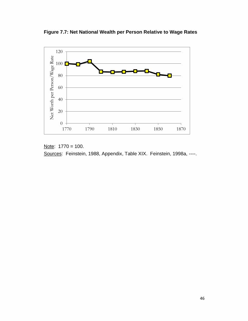
The work of Feinstein confirms the impression that wealth was, if

anything, declining relative to wage payments in Industrial Revolution

England. Figure 7.7 shows the net wealth per person in Britain, 1770-

1860, relative to the average earnings of full time workers, both as

estimated by Feinstein. Net wealth per person fell relative to the wage

rate by a full 20%, which is consistent with the Lindert data. Again, unless

returns to property were increasing in Industrial Revolution England, the

rising importance of wage income would have been an equalizing force in

the Industrial Revolution era.

Allen (2009), however, argues that returns to capital did increase

greatly in the Industrial Revolution period. What drives his conclusion is a

comparison of the growth rate of real wages versus the growth rate of

output per person in England in 1770-1870. The real wage estimated by

Charles Feinstein in 1770-1870 rises much less than the level of output

per person estimated by Crafts and Harley (Feinstein 1998a; Crafts and

Harley 1992). The inference is that, if output was rising faster than wages,

someone must have been receiving the benefits of that output, and given

that farmland rents declined as a share of output, it must have been the

capitalists. Marx and Engels were right when they wrote about the

increased polarization of the economy in the Communist Manifesto of

1848.

The ratio of the real wage to real output per person indicates the

movement of the share of labour in national income. Figure 7.8 shows the

shares of labour, capital, and land in national income estimated by Allen

(2009) in this way. In this picture the share of labour in total income falls

from around 60% in 1770 to less than 47% by the 1870. Over the same

22

interval the share of capital rises from 19% to 47%. Capital owners

appear as the big winners of the Industrial Revolution period compared to

both labourers and land owners.

As we saw, the net wealth per person relative to wages was declining

in 1770-1870 rather than increasing. So the increase in the estimated

share of capital in national income implies, in turn, that the profit rates on

capital must have sharply risen in 1770-1870. Taking capital stocks as

estimated by Feinstein, Allen estimates a rise in the gross return on capital

from circa 10% 1770-90 to 24% by 1870. This rise is shown in figure 7.9.

23

Figure 7.7 about here

Figure 7.8 about here

Figure 7.9 about here

But this raises a host of puzzles. The first of these is: where in the

economy did these extraordinary returns on capital appear? The

observed rate of return on many assets was very low in Industrial

Revolution Britain. The gross rate of return on traditional assets such as

farmland and housing remained low throughout the Industrial Revolution

era. The returns on holding farmland indeed had fallen to 3% or less by

1870. (Clark 1998, 2002.

It might be argued that high returns to capital would show up only

where innovation was more important, in the technologically transformed

sectors of the Industrial Revolution. However, railways, which Feinstein

reports contained one sixth of all fixed capital in Britain by 1860, 35 years

after their introduction, also typically generated low returns to investors

(Feinstein, 1988:452). Thus in the 1860s the average return on

investments in railways in the UK had already fallen to only 3.8%, and by

the 1870s that had dropped to 3.2% (Arnold and McCartney 2005: table 2;

Davis and Huttenback 1986: table 3.8).

Returns were low because, while initial railway investments often

proved profitable, even relatively modest initial profits induced a flood of

new entrants into the industry. By 1870 there were more than 12,000

miles of railway line in England alone. The ramification of the railway

network in 45 years into a dense net of competing lines created

substantial competition on all routes. Thus while, for example, the Great

Western controlled the direct line from London to Manchester, freight and

passengers could cross over from Manchester through other companies to

link up with the East Coast route to London. This kept rates low and

profits slim.

24

The engineering innovators who created the modern railway system

also benefitted only modestly. George Stephenson, for example, played

an enormous role in the development of the modern railway and was a

pioneer in the design of locomotives and steel rails and in the engineering

of lines. But he died in 1848 only modestly wealthy. He designed many

innovative locomotives, but there were always a host of competing

locomotive builders. His discovery through experiments at Killingworth

Colliery that even modest gradients absorbed much of the power of steam

locomotives was crucial to the design and engineering of the new railway

lines, such as the Liverpool and Manchester. But such knowledge was

not patentable innovation and was available to all his competitors.

In coal mining, another great Industrial Revolution industry, investors

again found slim returns. Coal output rose twenty fold between the 1700s

and the 1860s in England. Coal heated homes, made ore into iron,

brewed beer, and powered railway locomotives. Yet there were no

equivalents of the great fortunes made from oil in America’s late

nineteenth century industrialization. Good coal seams abounded, so the

rents for coal lands were always an extremely modest share of the price of

coal. And even as pits pushed ever deeper in search of rich coal seams,

the patentable innovation in the industry was modest, so coal owners

competed with each other on an equivalent basis. Competition between

such pits producing a homogenous output kept prices of coal low.

Consumers, not capitalists, were the great beneficiaries. The returns on

the capital embodied in sinking pits, in underground tramways, and in

winding gear all remained limited (Clark and Jacks 2007).

Even in the cotton textile industry, the heart of the Industrial

Revolution, returns on capital remained modest. Of the known textile

innovators, only a handful, such as Arkwright and the Peels, became

wealthy. Thus of the 379 people dying in the 1860s in Britain who left

estates of more than £0.5 million, only 17, 4%, were in textiles.4

(Rubinstein, 1981:79-92) .Yet the textile industry produced ten % of

national output in the early nineteenth century and a substantial fraction of

4

25

all growth in England 1760-1860 can be attributed to the efficiency gains

of the textile industry. Cotton textiles was characterized throughout the

Industrial Revolution by intense competition between thousands of modest

sized individual mills. This competition, at least in the early Industrial

Revolution, kept profits modest, in the order of 10% even for the most

innovative firms (Harley 1998).

If area after area of Industrial Revolution industry and enterprise had

extremely low returns on capital, for capital as a whole to have earned

nearly a nearly 25% rate of return by 1870 would require the remaining

sectors – shipping, retailing, brewing, gasworks – to have earned

extraordinary returns, many times even this 25%. These supernormal

returns should have produced a legion of wealthy entrepreneurs. Yet

Rubinstein’s survey of testators dying leaving £0.5 or more in personalty in

the later nineteenth century finds that the great majority of such estates

still came from those investing in the traditional sectors of land, banking or

law.

So what has gone wrong with Allen’s reasoning that leads to this

implausible account of fantastic gains for Industrial Revolution capital

owners, and ever widening income inequality? One problem is

conceptual. Allen compares the rise of the real purchasing power of

wages with the rise in the real value of output in the economy. But this is

not the right comparison. To see what happens to distribution, what

needs to be compared is the real purchasing power of wages with the real

purchasing power of output. In Industrial Revolution England there was a

significant difference between the gains in output and the gains in

purchasing power. As population increased, England switched from being

largely self-sufficient in food and other raw materials in the 1760s, to being

a substantial importer by the 1860s. These imports were paid for by huge

exports of textiles, iron, and coal. But the prices of these exports, spurred

by technological advances, fell substantially relative to the prices of

imports. This implies that many of the output gains of the Industrial

Revolution era were being exported to consumers of British textiles, iron

and coal around the world. They did not fall into the pockets of the

capitalist class.

26

Thus the output of the English economy rose much more than did the

purchasing power of the economy. This helps create the illusion that

output gains were much greater than the gains of the workers. But to

compare like with like, we should compare the rise in purchasing power of

workers with that of the other contributors to production, the land owners

and the capitalists. When the comparison is done on this basis, much of

the Allen puzzle disappears.

Another problem with this approach of comparing real wages to real

output per person is the question of what is the appropriate measure of

the real value of wages in the Industrial Revolution period. Allen and

Feinstein adopt a pessimistic deflator for wages compared to those used

by Lindert and Williamson and Clark, one that shows workers as facing an

ever rising cost of subsistence, despite the productivity gains of the era.

There is no simple demonstration that the pessimistic estimate of living

costs is better than the optimistic ones, since these differences are the

product of a variety of decisions on the weightings of items in the cost of

living and the appropriate prices to use.

Bread, for example, was the single most significant item of working

class consumption throughout this period. The ratio of bread prices to

wheat prices should be close to constant in the long run, given that wheat

constituted at least 80% of the cost of bread. The Feinstein series uses

bread prices in London as its measure of national bread prices. However,

London bread prices were regulated until 1815. When regulation ended

these London prices showed an abrupt upwards jump relative to wheat

prices of nearly 10%. If these London prices reflected a true price index

for bread of constant quality, then either London bakers after 1815 were

enjoying substantial and sustained profits, or before 1815 they suffered

from substantial and sustained losses. Given the competitive and small

scale nature of baking in this era, neither seems a plausible alternative.

The quality of bread in the absence of regulation must have improved, so

the nominal bread prices overstate the rise in the cost of living.

27

There is an alternative way of looking at the distribution of the gains of

the Industrial Revolution between workers and property owners, that

avoids this problem of what is the appropriate way of converting wages

and other earnings into real purchasing power. This is just to compare the

distribution of all earnings in the economy between workers, land owners,

and capital owners, in nominal terms without having to worry about what is

the correct price index. We can do this for the 1860s for wages using the

work of Leone Levi (1867). This suggests that all labour income for

England was then £411 million. The Property and Income Tax Returns of

1842 and later years provide estimates of the rental payments to land, and

the incomes of capital owners These returns distinguish income from

property of the following types: lands, houses, tithes, manors, fines,

quarries, mines, iron works, fisheries, canals, and railways. For the 1860s

the average of these reported incomes, reduced to the basis of England,

was £46 million for farmland rents, and £189 for housing and other forms

of capital income. This implies a labour share in all income of 64% in the

1860s, far in excess of the 47% that Allen infers should apply to 1870.

Based on estimates of the movement of wages, population, farmland

rents, coal land rents, house rents, and other returns on capital in earlier

years we can estimate the share of wages versus property income back to

the 1700s. (Clark 2010).These estimated shares are shown in figure 7.10.

As can be seen, the clear implication is that labour incomes were rising

modestly as a share of all incomes in England from 1700 to 1870: from

59% to 66%. Consequently distribution, measured just in terms of

nominal incomes, was shifting away from property owners and towards

workers.

The driver of this shift in distribution was the decline of farmland rents

as an important source of income. These fell from 21% of all incomes

circa 1700 to less than 7% circa 1870. The declining property incomes of

the land owners was only partially made up in greater property incomes

among capital owners, the share of capital in incomes rising from 21% to

27%.

28

Thus the various sources of evidence above present a consistent

picture: the Industrial Revolution did not result in any widening of income

and wealth inequalities in England. However great were the disruptions to

British society of technological shocks, population growth, urbanization,

and foreign trade in the years 1700-1870, inequalities of wealth and

income likely either stayed stable or declined in

Figure 7.10 about here

4. Conclusion

England underwent profound structural changes in 1770-1870. Rapid

population growth and technological advance led to the industrialization

and urbanization of the economy. Farming declined rapidly in

importance, and industrial and service activities correspondingly

increased. Capital was poured into new investments in canals, railways,

ports, mines, and urban infrastructure.

Yet we see that in terms of social mobility and income and wealth

inequality, none of this had much effect. The disruptions of the old

patterns of a heavily agrarian economy did not lead to a period of rapid

upward or downward social mobility. Mobility continued at the slow rates

of the pre-industrial economy and at the slow rates observed even to this

day.

Nor did the new economic opportunities generate extravagant returns

for investors. Capital was sufficiently abundant, and competition within

industries sufficiently vigorous, that the returns on capital remained

modest throughout these years. Indeed the declining relative value of

rents from farmland was not even fully compensated by increased profits

from urban capital goods within the economy. Thus the distribution of

income between property owners and workers actually changed in favour

of labour, though only by moderate amounts.

29

References

Allen, R.C. 2009. Engels’ pause: Technical change, capital accumulation,

and inequality in the British Industrial Revolution. Explorations in

Economic History, 46:418-435.

Arnold, A. J. and McCartney,. S. 2005. Rates of Return, Concentration

Levels, and Strategic Change in the British Railway Industry, 1830-1912.

Journal of Transport History 26:41-60.

Begg, I. and Henry, S.G.B. eds. 1998. Applied Economics and Public

Policy. Cambridge.

Cinnirella, F. 2008. Optimists or pessimists? A reconsideration of

nutritional status in Britain, 1740–1865. European Review of Economic

History 12:325–354.

Clark, G. 1998. Land Hunger: Land as a Commodity and as a Status

Good in England, 1500-1910., Explorations in Economic History, 35:59-

82.

Clark, G. 2002a. Farmland Rental Values and Agrarian History: England

and Wales, 1500-1912. European Review of Economic History, 6:281-

309.

Clark, G. 2005. The Condition of the Working-Class in England, 1209-

2004. Journal of Political Economy 113:1307-1340.

Clark, G. 2007. A Farewell to Alms: A Brief Economic History of the

World. Princeton.

Clark, G. 2010. The Macroeconomic Aggregates for England, 1209-2009.

Research in Economic History 27: 51-140.

Clark, G. and Cummins, N. 2012. What is the True Rate of Social

Mobility? Surnames and Social Mobility in England, 1800-2011. Working

Paper, University of California, Davis.

Clark, Gregory. 2002b. Shelter from the Storm: Housing and the

Industrial Revolution, 1550-1912. Journal of Economic History 62: 489-

511.

Crafts, N.F.R., and C. K. Harley. C. K. 1992. Output Growth and the

Industrial Revolution: A Restatement of the Crafts-Harley View. Economic

History Review 45:703-730.

30

Davis, L.E. and Huttenback. R.A. 1986. Mammon and the Pursuit of

Empire: the Economics of British Imperialism. Cambridge.

Delger, H., and J. Kok. 1998. Bridegrooms and biases: A critical look at

the study of intergenerational mobility on the basis of marriage certificates.

Historical Methods, 31 : 113-21.

Feinstein, C.H. 1995. Changes in Nominal Wages, the Cost of Living and

Real Wages in the United Kingdom over Two Centuries.” Iin P Scholliers,

P and V. Zamagni, V. (eds.),1995,

Feinstein, C.H., 1988. “National Statistics, 1760-1920.” In Feinstein,

C.H.and Sidney Pollard, S. (eds.) 1988.

Feinstein, C.H., 1998a. Wage-earnings in Great Britain during the

industrial revolution. In: Begg, I. and Henry, S.G.B. eds, 1998.

Feinstein, C.H.and Pollard, S. eds. 1988. Studies in Capital Formation in

the United Kingdom, 1750-1920. Oxford.

Feinstein, CH., 1998b. Pessimism Perpetuated: real wages and the

standard of living in Britain during and after the industrial revolution.

Journal of Economic History 58:,625–658.

Goldthorpe, J. H. 1987. Social Mobility and Class Structure in Modern

Britain. Oxford.

Harley, C.K. 1998. Cotton Textile Prices and the Industrial Revolution.

Economic History Review, 51:49-83.

Humphries, J. 2010. Childhood and Child Labour in the Industrial

Revolution. Cambridge.

Levi, L. 1867. Wages and Earnings of the Working Classes.

Lindert, P.H. 1986. Unequal English Wealth since 1670., Journal of

Political Economy, 94:1127-62.

Lindert, P.H. and Williamson, J.G. 1983. English Workers’ Living

Standards during the Industrial Revolution: A New Look. Economic History

Review, 36:1-25

Lindert, P.H. and Williamson, J.G. 1985. English Workers’ Real Wages:

Reply to Crafts. Journal of Economic History, 45:145-53.

Long, J. 2013 forthcoming. Social Mobility within and across Generations

in Britain since 1851. European Review of Economic History ,17.

31

Miles, A. 1999. Social Mobility in Nineteenth- and Early Twentieth-

Century England. New York.

Mitch, D. 1993. “Inequalities which everyone may remove”: Occupational

recruitment, endogamy, and the homogeneity of social origins in Victorian

England in Building European society: Occupational change and social

mobility in Europe, edited by A. Miles and D. Vincent, 14044. Manchester:

Manchester University Press.

Mokyr, J. 1988. Is There Still Life in the Pessimist Case? Consumption

during the Industrial Revolution, 1790-1850. Journal of Economic History,

48:69-92.

Rubinstein, W. D. 1981. Men of Property: The Very Wealthy in Britain

Since the Industrial Revolution.

Sanderson, M. 1972. Literacy and Social Mobility in the Industrial

Revolution in England. Past & Present, 56:75-104.

Scholliers, P and Zamagni, V. eds.,1995. Labour’s Reward: Real Wages

and Economic Change in 19th- and 20th-Century Europe. Aldershot.

Stamp, J. 1922. British Incomes and Property.

United Kingdom, H.M. Revenue and Customs. 2007. Distribution of

Wealth, 2003.

United Kingdom, Office of National Statistics. 2006. Annual Survey of

Hours and Earnings.

Williamson, J.G., 1985. Did British Capitalism Breed Inequality? Boston.

32

Table 7.1: Intergenerational Mobility in England, 1854-1874, from

Marriage Registers

Father’s Class

I II III IV V Son’s Class

I 54 4 0 0 0

II 30 53 6 5 3

III 7 23 75 33 20

IV 5 10 8 47 12

V 5 10 10 15 65

Notes: The columns show the %age of the sons of fathers of each

occupational class by their occupational class. Source: Miles, 1999, table

2.3 (N=2,483).

Table 7.2: Intergenerational Mobility in Britain, 1851-1881, from Long

Father’s Class

I II III IV V Son’s Class

I 35 5 3 1 1

II 21 35 10 6 7

III 36 46 68 38 56

IV 2 9 8 38 15

V 6 6 11 17 21

Note: Sons aged 0-19 in 1851. The columns show the %age of the sons

of fathers of each occupational class by their occupational class. Source:

Long, 2013, table 2, (N=12,516).

33

Figure 7.1: The Extremes of Mobility Illustrated

0.0

0.2

0.4

0.6

0.8

1.0

0.0 0.2 0.4 0.6 0.8 1.0

So

n's

Sta

tus

Father's Status

b = 0

0.0

0.2

0.4

0.6

0.8

1.0

0.0 0.2 0.4 0.6 0.8 1.0

So

n's

Sta

tus

Father's Status

b = 1

34

Figure 7.2: Intergenerational Occupational Mobility Compared

Notes: Social Class has been assigned a status from 0 to 1, based on the

average earnings of each social class, as estimated by Long, 2013.

Sources: Tables 1-3, and earnings by occupation from Long, 2013, table

9.

0.0

0.2

0.4

0.6

0.8

1.0

0.0 0.2 0.4 0.6 0.8 1.0

So

cial

Cla

ss S

on

Social Class Father

1851-81

1972

45 Degree

Marriage 1859-74

35

Table 7.3: Intergenerational Mobility in Britain in 1972

Father’s Class

I II III IV V Son’s Class

I 32 9 6 3 2

II 42 41 24 16 10

III 23 36 52 56 55

IV 4 12 15 22 24

V 0 3 3 3 8

Note: Sons aged 30-49 in 1972, father’s occupation when son was 14.

Source: Goldthorpe, 1987, as reported in Long, 2013, table 8. (N=3,460).

36

Figure 7.3: Change in Relative Representation and b

Note: For clarity the vertical scale is logarithmic.

1

2

4

8

16

0 1 2 3 4 5

Re

lative

Re

pre

se

nta

tio

n

Generation

b = .25

b = .5

b = .75

37

Table 7.4: Relative Representation of Rare Surnames by Period and

Cohort

Generation

Clark(e)

1680-

1709

Sample

1710-39

Sample

1740-69

Sample

1770-99

Sample

1710-39 1.13 1740-69

1.13 4.18

1770-99 1.06

3.18 6.28

1800-29 1.22

3.09 5.03 6.36

1830-58 1.13

2.24 4.06 4.92 6.22

Notes: The relative representation of these surnames in each period is

measures as their share among PCC wills compared to their share of

marriages in England.

38

Figure 7.4: Relative Representation of Cohorts of Elite Surnames in

the PCC, England, 1710-1858

Note: The vertical axes is on a logarithmic scale, so that a constant rate

of decline of relative representation would appear as a straight line.

1

2

4

8

1710 1740 1770 1800 1830 1860

Rel

ativ

e R

epre

sen

tati

on

1680-1709

1710-39

1740-69

1770-99

Clark

39

Table 7.5: Implied bs, England, 1710-1858, Downward Mobility

Generation

1680-

1709

Sample

1710-39

Sample

1740-69

Sample

1770-99

Sample

Average

1740-69 0.77

0.77

1770-99 0.97

0.84 0.90

1800-29 0.68

0.83 0.81 0.78

1830-58 0.86

0.88 0.88 0.83 0.86

Average 0.82

0.85 0.85 0.83 0.82

40

Table 7.6: Wealth b Inferred from the Proportion Probated, 1888-2011

Generation

Rich

1858-1887

Prosperous

1858-1887

Average by

period

1888-1917 0.70 0.87 0.78

1918-1952 0.74 0.79 0.77

1953-1989 0.59 0.48 0.54

1990-2011a 0.68 0.91 0.79

Average

0.68

0.76

0.72

Note: ab estimate adjusted down to reflect incomplete generation

observed.

41

Figure 7.5: Relative Representation of Rare Elite Surnames in earlier

Generations, England, 1680-1829

1

2

4

8

1680 1710 1740 1770 1800 1830

Rel

ativ

e R

epre

sen

tati

on

1740-69

1770-99

1800-29

1830-59

Clark

42

Table 7.7: Implied bs, England, 1710-1858, Upward Wealth Mobility

Generation

1740-69

Sample

1770-99

Sample

1800-29

Sample

1830-58

Sample

Average

1710-39 0.61

0.68 0.65 0.67 0.65

1740-69

0.86 0.83 0.83 0.84

1770-99

0.84 0.83 0.83

1800-29

0.77 0.77

Average 0.61

0.77 0.77 0.77 0.77

43

Figure 7.6: Relative Representation and Implied bs at Oxbridge, 1530-

2012

Note: The circles indicate the observations for the wealthy surnames, the

squares those for the rare surnames appearing at Oxford and Cambridge

1800-29.

Source: See Clark and Cummins, 2012.

1

2

4

8

16

32

64

1530 1590 1650 1710 1770 1830 1890 1950 2010

Rel

ativ

e R

epre

sen

tati

on

b = 0.77 b = 0.77

b = 0.82

b = 0.83

44

Table 7.8: Wealth Distribution in England, 1700-1875 from Lindert

1700

1740

1810

1875

Share - Top 1% 39 44 55 61

Share - Top 10% 81 86 83 84

Net Worth per Person

(£ )

58 95 247 279

Average Male Wage

(d./day)

13.4 14.4 34.4 49.7

Net Worth Relative to

the Wage (1740 = 100)

66

100

109

85

Source: Lindert, 1986, tables 1, 4. Male Wage, 1700, 1740, 1810, Clark,

2010. Male wage 1875 from Feinstein, 1998a (matched to Clark series

based on 1860-69).

45

Table 7.9: Distribution of Wages and Wealth, UK, 2003-4

Decile

Share of wages

(%)

Share of net

assets

(%)

90-100 26.3 44.6

80-90 14.2 16.2

70-80 11.5 10.3

60-70 10.0 9.7

50-60 8.7 7.9

40-50 7.7 5.3

30-40 6.7 3.5

20-30 5.8 1.8

10-20 4.9 0.1

0-10 4.2 0.0

Source: United Kingdom, Office of National Statistics, 2006. United

Kingdom, H. M. Revenue and Customs, 2007, table 13.1. Note: Wages

for full-time adult workers. Wealth from the assets of those dying 2003.

46

Figure 7.7: Net National Wealth per Person Relative to Wage Rates

Note: 1770 = 100.

Sources: Feinstein, 1988, Appendix, Table XIX. Feinstein, 1998a, ----.

0

20

40

60

80

100

120

1770 1790 1810 1830 1850 1870

Net

Wo

rth

per

Per

son

/W

age

Rat

e

47

Figure 7.8: Allen estimate of factor shares, 1770-1870.

Source: Allen, 2009, figure 2.

0.0

0.2

0.4

0.6

0.8

1.0

1770 1790 1810 1830 1850 1870

Sh

ares

of

Nat

ion

al I

nco

me

Labor

Capital

Land

48

Figure 7.9: Allen’s Estimated Gross Profit Rates on Capital

Source: Allen, 2009, figure 3. The profit rate is measured relative to

Feinstein’s estimated “real capital stock” (Allen, 2009, 421). It is clear this

is a gross stock,

0

5

10

15

20

25

1770 1790 1810 1830 1850 1870

Rat

e o

f R

eturn

on

Cap

ital

(%

)

49

Figure 7.10: Shares of Capital, Land and Labour in Income, 1700-

1870

Source: Clark, 2010.

1700 1720 1740 1760 1780 1800 1820 1840 1860

Sh

are

of

Inco

me Farmland

Capital

Labor