CHAPTER 7 Applications of Integration -...
50
CHAPTER 7 Applications of Integration Section 7.1 Area of a Region Between Two Curves . . . . . . . . . . 313 Section 7.2 Volume: The Disk Method . . . . . . . . . . . . . . . . . 321 Section 7.3 Volume: The Shell Method . . . . . . . . . . . . . . . . 328 Section 7.4 Arc Length and Surfaces of Revolution . . . . . . . . . . 335 Section 7.5 Work . . . . . . . . . . . . . . . . . . . . . . . . . . . . 341 Section 7.6 Moments, Centers of Mass, and Centroids . . . . . . . . . 344 Section 7.7 Fluid Pressure and Fluid Force . . . . . . . . . . . . . . . 350 Review Exercises . . . . . . . . . . . . . . . . . . . . . . . . . . . . . 353 Problem Solving . . . . . . . . . . . . . . . . . . . . . . . . . . . . . . 359
Transcript of CHAPTER 7 Applications of Integration -...

C H A P T E R 7Applications of Integration
Section 7.1 Area of a Region Between Two Curves . . . . . . . . . . 313
Section 7.2 Volume: The Disk Method . . . . . . . . . . . . . . . . . 321
Section 7.3 Volume: The Shell Method . . . . . . . . . . . . . . . . 328
Section 7.4 Arc Length and Surfaces of Revolution . . . . . . . . . . 335
Section 7.5 Work . . . . . . . . . . . . . . . . . . . . . . . . . . . . 341
Section 7.6 Moments, Centers of Mass, and Centroids . . . . . . . . . 344
Section 7.7 Fluid Pressure and Fluid Force . . . . . . . . . . . . . . . 350
Review Exercises . . . . . . . . . . . . . . . . . . . . . . . . . . . . . 353
Problem Solving . . . . . . . . . . . . . . . . . . . . . . . . . . . . . . 359

313
C H A P T E R 7Applications of Integration
Section 7.1 Area of a Region Between Two Curves
1. A � �6
0�0 � �x2 � 6x�� dx � ��6
0�x2 � 6x� dx 3.
� �3
0��2x2 � 6x� dx
A � �3
0 ���x2 � 2x � 3� � �x2 � 4x � 3�� dx
5.
or �6�1
0 �x3 � x� dx
A � 2�0
�1 3�x3 � x� dx � 6�0
�1 �x3 � x� dx
7.
5
4
3
2
1
542 31x
y
�4
0 ��x � 1� �
x2� dx 9.
6
5
3
2
654321
1
x
y
�6
0 �4�2�x�3� �
x6� dx 11.
x
y
3
−13 3
π3
2π3
2π π
���3
���3 �2 � sec x� dx
13. (a)
Intersection points: and
(b) A � �2
�3 ��4 � y2� � �y � 2�� dy �
1256
A � �0
�5 ��x � 2� � 4 � x dx � �4
024 � x dx �
616
�323
�1256
��5, �3��0, 2�
�y � 3��y � 2� � 0
y2 � y � 6 � 0
4 � y2 � y � 2
x � y � 2
x−6 −4 6
−6
4
6
(−5, −3)
(0, 2)
y x � 4 � y2
15.
Matches (d)
A 4
g�x� � �x � 1�2
x1 2 3
2
3
(0, 1)
(3, 4)
yf �x� � x � 1

314 Chapter 7 Applications of Integration
19. The points of intersection are given by:
�323
� ��x3
3� 2x2�
4
0
� ��4
0 �x2 � 4x� dx
x(4, 0)(0, 0)
1 2 3 5−1
−2
−3
−4
−5
y A � �4
0 �g�x� � f �x�� dx
x�x � 4� � 0 when x � 0, 4
x2 � 4x � 0
21. The points of intersection are given by:
� �2x �x2
2�
x3
3 �2
�1�
92
10
6
4
21234
8), 9(2
x
)01,(
y � �2
�1 �2 � x � x2� dx
� �2
�1 ��3x � 3� � �x2 � 2x � 1�� dx
A � �2
�1 �g�x� � f �x�� dx
�x � 2��x � 1� � 0 when x � �1, 2
x2 � 2x � 1 � 3x � 3
23. The points of intersection are given by:
Note that if we integrate with respect to we need two integrals. Also, note that the region is a triangle.
x,
A � �1
0 ��2 � y� � �y�� dy � �2y � y2�
1
0� 1
x � 1 x � 0 x � 2
x � 2 � x and x � 0 and 2 � x � 0
32
3
1
2
)1,1
x)0,2(
0),0(
(
y
17.
� �168
�42
� 2� � 0 � 2
� �x4
8�
x2
2� x�
2
0
� �2
0 �1
2x3 � x � 1� dx
6
5
4
3
43−2 1
1
x
y
(0, 1)
(0, 2)
(2, 6)
(2, 3)
A � �2
0 ��1
2x3 � 2� � �x � 1�� dx
25. The points of intersection are given by:
� �29
�3x�3�2 �x2
2 �3
0�
32
5
3
2
4
1 2−2 3 4x
), 4(3
0( 1, )
y � �3
0 ��3x�1�2 � x� dx
� �3
0 ��3x � 1� � �x � 1�� dx
A � �3
0 � f �x� � g�x�� dx
3x � x when x � 0, 3
3x � 1 � x � 1
27. The points of intersection are given by:
� �2y �y2
2�
y3
3 �2
�1�
92
� �2
�1 ��y � 2� � y2� dy
3
2
1
542 31
1
3
, 2)(4
x
1, )(1
y A � �2
�1 �g�y� � f �y�� dy
�y � 2��y � 1� � 0 when y � �1, 2
y2 � y � 2
Section 7.1 Area of a Region Between Two Curves 315
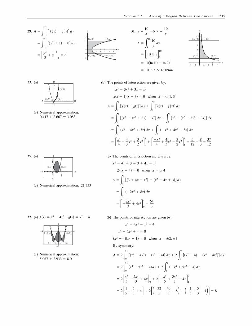
29.
� �y3
3� y�
2
�1� 6
� �2
�1 ��y2 � 1� � 0� dy
64 5
3
1
32
2
x
y
(0, −1)
(0, 2) (5, 2)
(2, −1)
A � �2
�1 � f �y� � g�y�� dy 31.
� 10 ln 5 16.0944
� 10�ln 10 � ln 2�
� �10 ln y�10
2
A � �10
2 10y
dy
12
8
6
864−4 −2 2
4
x
y
(1, 10)(0, 10)
(5, 2)(0, 2)
y �10x
⇒ x �10y
33. (a)
(c) Numerical approximation:0.417 � 2.667 3.083
−6 12
−1
(3, 9)
(1, 1)(0, 0)
11 (b) The points of intersection are given by:
� �x4
4�
43
x3 �32
x2�1
0� ��x4
4�
43
x3 �32
x2�3
1�
512
�83
�3712
� �1
0 �x3 � 4x2 � 3x� dx � �3
1 ��x3 � 4x2 � 3x� dx
� �1
0 ��x3 � 3x2 � 3x� � x2� dx � �3
1 �x2 � �x3 � 3x2 � 3x�� dx
A � �1
0 � f �x� � g�x�� dx � �3
1 �g�x� � f �x�� dx
x�x � 1��x � 3� � 0 when x � 0, 1, 3
x3 � 3x2 � 3x � x2
35. (a)
(c) Numerical approximation: 21.333
(4, 3)(0, 3)
−6 12
−3
9 (b) The points of intersection are given by:
� ��2x3
3� 4x2�
4
0�
643
� �4
0 ��2x2 � 8x� dx
A � �4
0 ��3 � 4x � x2� � �x2 � 4x � 3�� dx
2x�x � 4� � 0 when x � 0, 4
x2 � 4x � 3 � 3 � 4x � x2
37. (a)
(c) Numerical approximation:5.067 � 2.933 � 8.0
−4 4
−5
2
(−2, 0) (2, 0)
(−1, −3) (1, −3)
f �x� � x4 � 4x2, g�x� � x2 � 4 (b) The points of intersection are given by:
By symmetry:
� 2� 15
�53
� 4� � 2���325
�403
� 8� � ��15
�53
� 4�� � 8
� 2�x5
5�
5x3
3� 4x�
1
0� 2��x5
5�
5x3
3� 4x�
2
1
� 2 �1
0 �x4 � 5x2 � 4� dx � 2 �2
1 ��x4 � 5x2 � 4� dx
A � 2 �1
0 ��x4 � 4x2� � �x2 � 4�� dx � 2 �2
1 ��x2 � 4� � �x4 � 4x2�� dx
�x2 � 4��x2 � 1� � 0 when x � ±2, ±1
x4 � 5x2 � 4 � 0
x4 � 4x2 � x2 � 4
316 Chapter 7 Applications of Integration
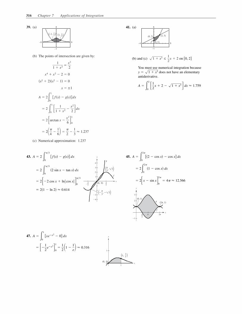
39. (a)
(b) The points of intersection are given by:
(c) Numerical approximation: 1.237
� 2��
4�
16� �
�
2�
13
1.237
� 2 �arctan x �x3
6 �1
0
� 2 �1
0 � 1
1 � x2 �x2
2 � dx
A � 2�1
0 � f �x� � g�x�� dx
x � ±1
�x2 � 2��x2 � 1� � 0
x4 � x2 � 2 � 0
1
1 � x2 �x2
2
−3 3
−1
−1, 12 1, 1
2( (( (
3 41. (a)
(b) and (c) on
You must use numerical integration becausedoes not have an elementary
antiderivative.
A � �2
0 �1
2x � 2 � 1 � x3� dx 1.759
y � 1 � x3
�0, 2�1 � x3 ≤12
x � 2
−4 5
−1
(0, 2)
(0, 1)
(2, 3)
5
43.
� 2�1 � ln 2� 0.614
� 2��2 cos x � ln cos x ���3
0
� 2 ���3
0 �2 sin x � tan x� dx
2
3
4
1
2
2
3
4
3,3
x
y
0)0,(
3,3
g
f
π
π
ππ
A � 2 ���3
0 � f �x� � g�x�� dx 45.
x
y
2
3
−1
ππ
π
π2
2
g
f
(2 , 1)
(0, 1)
� 2�x � sin x�2�
0� 4� 12.566
� 2�2�
0�1 � cos x� dx
A � �2�
0��2 � cos x� � cos x� dx
47.
� ��12
e�x2�1
0�
12 �1 �
1e� 0.316
A � �1
0 �xe�x2
� 0� dx
1
x
,,
1
)0( ,0
1( )
y
1e

Section 7.1 Area of a Region Between Two Curves 317
51. (a)
060
4
(1, e)
(3, 0.155)
(b)
� e � e1�3
� ��e�1�x�3
1
A � �3
1 1x2 e1�x dx (c) Numerical approximation: 1.323
53. (a)
−1
−1
4
6 (b) The integral
does not have an elementaryantiderivative.
A � �3
0 x3
4 � x dx
(c) A 4.7721
55. (a) 5
3
−1
−3
(b) The intersection points are difficult to determine by hand.
(c) where
c 1.201538.
Area � �c
�c
�4 cos x � x2� dx 6.3043
49. (a)
00
3
�
(b)
� �2 �12� � ��2 �
12� � 4
� ��2 cos x �12
cos 2x��
0
A � ��
0�2 sin x � sin 2x� dx (c) Numerical approximation: 4.0
57. F�x� � �x
0 �1
2t � 1� dt � �t 2
4� t�
x
0�
x2
4� x
(a)
t
4
y
5
6
2
3
−1−1 1 2 3 4 5 6
F�0� � 0 (b)
t
4
y
5
6
2
3
−1−1 1 2 3 4 5 6
F�2� �22
4� 2 � 3 (c)
t
4
y
5
6
2
3
−1−1 1 2 3 4 5 6
F�6� �6 2
4� 6 � 15
59. F ��� � ��
�1cos
��
2 d� � � 2
� sin
��
2 ��
�1�
2�
sin ��
2�
2�
(a)
y
1
32
12
12
−
12
12
−θ
F ��1� � 0 (b)
y
1
32
12
12
−
12
12
−θ
F �0� �2�
0.6366 (c)
y
1
32
12
12
−
12
12
−θ
F�12� �
2 � 2�
1.0868

318 Chapter 7 Applications of Integration
61.
� � 74
x2 � 7x�4
2� ��7
4x2 � 21x�
6
4� 7 � 7 � 14
� �4
2 � 7
2x � 7� dx � �6
4 ��7
2x � 21� dx
(4, 6)
(6, 1)
(2, 3)−y x= 5−
52y x= + 16−
92y x= 12−y
x2 6 8 10
−4
−2
2
4
6
A � �4
2 �� 9
2x � 12� � �x � 5�� dx � �6
4 ���5
2x � 16� � �x � 5�� dx
63. Left boundary line:
Right boundary line:
� �2
�24 dy � 4y�
2
�2� 8 � ��8� � 16
A � �2
�2 �� y � 2� � � y � 2�� dy
y � x � 2 ⇔ x � y � 2
x
y
−1−2−4 2 3 4
−3
−4
1
2
3
4
(4, 2)(0, 2)
(0, −2)(−4, −2)
y � x � 2 ⇔ x � y � 2
67.
At
Tangent line: or
The tangent line intersects at
A � �1
�2 �x3 � �3x � 2�� dx � �x4
4�
3x2
2� 2x�
1
�2�
274
x � �2.f �x� � x3
y � 3x � 2y � 1 � 3�x � 1�
f � �1� � 3.�1, 1�,
f��x� � 3x2
(1, 1)
( 2, 8)− −
x1 2 3 4−2−3−4
−6
−8
2
4
6
8
y x= 3 2−
f x x( ) = 3
y f �x� � x3
65. Answers will vary. If you let and
(a)
(b)
� 2�502� � 1004 sq ft
Area 60
3�10� �0 � 4�14� � 2�14� � 4�12� � 2�12� � 4�15� � 2�20� � 4�23� � 2�25� � 4�26� � 0�
� 3�322� � 966 sq ft
Area 60
2�10� �0 � 2�14� � 2�14� � 2�12� � 2�12� � 2�15� � 2�20� � 2�23� � 2�25� � 2�26� � 0�
n � 10, b � a � 10�6� � 60.�x � 6
69.
At
Tangent line: or
The tangent line intersects at
A � �1
0 � 1
x2 � 1� ��1
2 x � 1�� dx � �arctan x �
x2
4� x�
1
0�
� � 34
0.0354
x � 0.f �x� �1
x2 � 1
y � �12
x � 1y �12
� �12
�x � 1�
f � �1� � �12
.�1, 12�,
f � �x� � �2x
�x2 � 1�2
x1 2
(0, 1)
1,
12
12
14
32
34
( )
f x( ) =1
2x + 1
12
12
y x= + 1−
y f �x� �1
x2 � 1

Section 7.1 Area of a Region Between Two Curves 319
71. on
You can use a single integral because on ��1, 1�.1 � x2x 4 � 2x2 � 1 ≤
� �x3
3�
x5
5 �1
�1�
415
� �1
�1 �x2 � x 4� dx
A � �1
�1 ��1 � x2� � �x 4 � 2x2 � 1�� dx
)x
2
10, )(
,(10)1( , 0
y��1, 1�x 4 � 2x2 � 1 ≤ 1 � x2
73. Offer 2 is better because the accumulated salary (area under the curve) is larger.
75.
b � 9 �9
34 3.330
9 � b �9
34
�9 � b�3�2 �272
23
�9 � b�3�2 � 9
��9 � b�x �x3
3 �9�b
0� 9
�9�b
0 ��9 � b� � x2� dx � 9
�9�b
�9�b
��9 � x2� � b� dx � 18
10
6
2
4
226
6
x
,, b9 b ),,( 9 bb ) (
y A � �3
�3 �9 � x2� dx � 36 77. Area of triangle is
Since select
y
x
a
21 3 4
1
2
3
B
O
A
a � 4 � 22 1.172.0 < a < 4,
a � 4 ± 22
a2 � 8a � 8 � 0
4 � �a
0�4 � x� dx � �4x �
x2
2 �a
0� 4a �
a2
2
12�4��4� � 8.OAB
79.
where and is the same as
�1
0 �x � x2� dx � �x2
2�
x3
3 �1
0�
16
.
�x �1n
xi �in
x( 01, )
2x xf )x(
.0 8.0 6...
0)
02
(0
0
,
4 1.0
0.
0.
.0
6
4
2
ylim
���→0 �
n
i�1 �xi � xi
2� �x
81. �5
0 ��7.21 � 0.58t� � �7.21 � 0.45t�� dt � �5
0 0.13t dt � �0.13t2
2 �5
0� $1.625 billion
83. (a)
(c) billion dollars
(Answers will vary.)
Surplus � �17
12� y1 � y2� dt 926.4
t
R
Rec
eipt
s (i
n bi
llion
s)
Time (in years)2 4 6 8 10 12
100
200
300
400
500
600
y1 � �270.3151��1.0586�t � 270.3151e0.05695t (b)
(d) No, forever because No, these models are not accurate for the future.According to news, eventually.E > R
1.0586 > 1.0416.y1 > y2
t
E
Exp
endi
ture
s (i
n bi
llion
s)
Time (in years)2 4 6 8 10 12
100
200
300
400
500
600
y2 � �239.9704��1.0416�t � 239.9704e0.04074t

320 Chapter 7 Applications of Integration
85. 5%:
Difference in profits over 5 years:
Note: Using a graphing utility, you obtain $193,183.
893,000�0.2163� $193,156
893,000��25.6805 � 34.0356� � �20 � 28.5714��
�5
0 �893,000e0.05t � 893,000e0.035t� dt � 893,000�e0.05t
0.05�
e0.035t
0.035�5
0
P2 � 893,000e�0.035�t312%:
P1 � 893,000e�0.05�t
87. The curves intersect at the point where the slope of equals that of
y2 � 0.08x2 � k ⇒ y�2 � 0.16x � 1 ⇒ x �1
0.16� 6.25
y1, 1.y2
(a) The value of k is given by
k � 3.125.
6.25 � �0.08��6.25�2 � k
y1 � y2
(b)
� 2�6.510417� 13.02083
� 2�0.08x3
3� 3.125x �
x2
2 �6.25
0
� 2 �6.25
0 �0.08x2 � 3.125 � x� dx
Area � 2 �6.25
0 �y2 � y1� dx
91. True89. (a)
(b)
(c) 5000V 5000�11.816� � 59,082 pounds
V � 2A 2�5.908� 11.816 m3
A 6.031 � 2�� � 116�
2
� � 2�� �18�
2
� 5.908
93. Line:
x
1
−1
(0, 0)
12
y
4 3
7 6
12
π
π 6π
, −( (
2.7823
�32
�7�
24� 1
� ��cos x �3x2
14��7��6
0
A � �7��6
0 �sin x �
3x7�� dx
y ��37�
x 95. We want to find such that:
But, because is on the graph.
x
(b, c)c
y = 2x − 3x3
y
c �49
b �23
9b2 � 4
4 � 3b2 � 8 � 12b2 � 0
b2 �34b4 � �2b � 3b3�b � 0
�b, c�c � 2b � 3b3
b2 �34b4 � cb � 0
�x2 �34 x 4 � cx�
b
0� 0
�b
0��2x � 3x3� � c� dx � 0
c
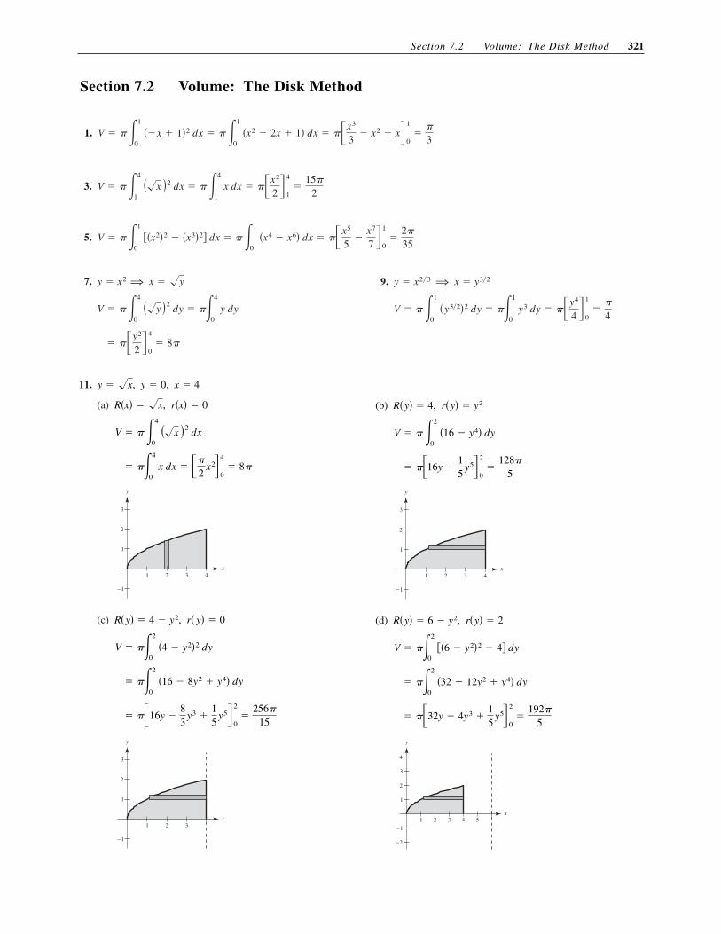
Section 7.2 Volume: The Disk Method 321
Section 7.2 Volume: The Disk Method
1. V � � �1
0 ��x � 1�2 dx � � �1
0 �x2 � 2x � 1� dx � ��x3
3� x2 � x�
1
0�
�
3
3. V � � �4
1 ��x �2 dx � � �4
1 x dx � ��x2
2 �4
1�
15�
2
5. V � � �1
0 ��x2�2 � �x3�2� dx � � �1
0 �x4 � x6� dx � ��x5
5�
x7
7 �1
0�
2�
35
7.
� ��y2
2 �4
0� 8�
V � � �4
0 ��y �2 dy � ��4
0 y dy
y � x2 ⇒ x � �y 9.
V � � �1
0 �y32�2 dy � ��1
0 y3 dy � ��y4
4 �1
0�
�
4
y � x23 ⇒ x � y32
11.
(a)
(c)
x1 2 3
−1
1
2
3
y
� ��16y �83
y3 �15
y5�2
0�
256�
15
� ��2
0 �16 � 8y2 � y4� dy
V � ��2
0 �4 � y2�2 dy
r� y� � 0R�y� � 4 � y2,
x1 2 3 4
−1
1
2
3
y
� ��4
0 x dx � ��
2x2�
4
0� 8�
V � � �4
0 ��x �2 dx
r�x� � 0R�x� � �x,
x � 4y � 0,y � �x,
(b)
(d)
x1 2 3 4 5
−2
−1
1
2
3
4
y
� ��32y � 4y3 �15
y5�2
0�
192�
5
� ��2
0 �32 � 12y2 � y4� dy
V � ��2
0 ��6 � y2�2 � 4� dy
r�y� � 2R�y� � 6 � y2,
x1 2 3 4
−1
1
2
3
y
� ��16y �15
y5�2
0�
128�
5
V � � �2
0 �16 � y4� dy
r�y� � y2R�y� � 4,
322 Chapter 7 Applications of Integration
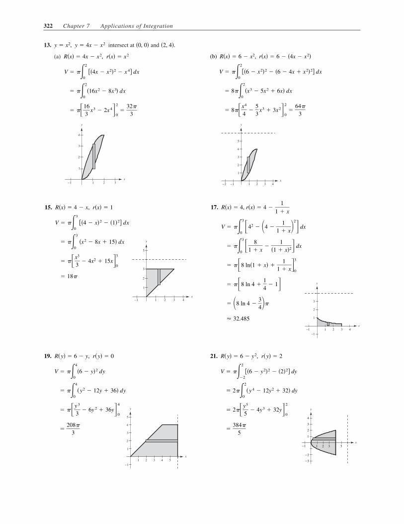
13. intersect at and
(a)
x
1
2
3
4
−1 1 2 3
y
� ��163
x3 � 2x 4�2
0�
32�
3
� ��2
0�16x2 � 8x3� dx
V � ��2
0 ��4x � x2�2 � x 4� dx
r�x� � x2R�x� � 4x � x2,
�2, 4�.�0, 0�y � 4x � x2y � x2,
(b)
x−2 −1 1 2 3 4
1
2
3
4
5
y
� 8��x4
4�
53
x3 � 3x2�2
0�
64�
3
� 8��2
0�x3 � 5x2 � 6x� dx
V � ��2
0��6 � x2�2 � �6 � 4x � x2�2� dx
r�x� � 6 � �4x � x2�R�x� � 6 � x2,
15.
� 18�
� ��x3
3� 4x2 � 15x�
3
0
x−1 1 2 3 4
1
2
3
5
y � ��3
0 �x2 � 8x � 15� dx
V � ��3
0 ��4 � x�2 � �1�2� dx
r�x� � 1R�x� � 4 � x, 17.
32.485
� �8 ln 4 �34��
1
1−1−1
2 3 4
2
3
y
x
� ��8 ln 4 �14
� 1�
� ��8 ln�1 � x� �1
1 � x�3
0
� ��3
0 � 8
1 � x�
1�1 � x�2� dx
V � ��3
0 �42 � �4 �
11 � x�
2
� dx
R�x� � 4, r�x� � 4 �1
1 � x
19.
�208�
3
x1 2 3 4 5
1
−1
2
3
4
5
y � ��y 3
3� 6y 2 � 36y�
4
0
� ��4
0�y2 � 12y � 36� dy
V � ��4
0�6 � y�2 dy
r�y� � 0R�y� � 6 � y, 21.
�384�
5
−1 5321
−2
−3
1
2
3
4
x
y � 2��y5
5� 4y3 � 32y�
2
0
� 2��2
0�y 4 � 12y2 � 32� dy
V � ��2
�2��6 � y2�2 � �2�2� dy
r�y� � 2R�y� � 6 � y2,

Section 7.2 Volume: The Disk Method 323
23.
x1 2 3
−1
1
2
y
� � ln 4 4.355
� �� ln x � 1 �3
0
� ��3
0
1x � 1
dx
V � ��3
0 � 1�x � 1�
2
dx
r�x� � 0R�x� �1
�x � 1, 25.
x1 2 3 4
−1
−2
1
2
y
�3�
4
� ���1x�
4
1
V � ��4
1 �1
x�2
dx
r�x� � 0R�x� �1x
, 27.
x1 2
1
2
y
��
2�1 � e�2� 1.358
� ���
2e�2x�
1
0
� ��1
0 e�2x dx
V � ��1
0�e�x�2 dx
r�x� � 0R�x� � e�x,
29.
The curves intersect at and
� �1523
� �125
3�
277�
3
� ���x 4 �83
x3 � 10x2 � 24x�2
0� ��x 4 �
83
x3 � 10x2 � 24x�3
2
� ��2
0��4x3 � 8x2 � 20x � 24� dx � ��3
2�4x3 � 8x2 � 20x � 24� dx
2
2 3 41−1−2
6
8
10
y
x
(2, 5)
V � ��2
0��5 � 2x � x2�2 � �x2 � 1�2�� dx � ��3
2��x2 � 1�2 � �5 � 2x � x2�2� dx
�2, 5�.��1, 2�
�x � 2��x � 1� � 0
x2 � x � 2 � 0
2x2 � 2x � 4 � 0
x2 � 1 � �x2 � 2x � 5
31.
� 8� �13
�r2h, Volume of cone
��
9�216 � 216 �2163 �
��
9�36y � 6y2 �y3
3 �6
0
��
9�6
0�36 � 12y � y2� dy
V � ��6
0 �1
3 �6 � y��
2
dy
x1 3 4 5 6
1
2
3
4
5
6
yy � 6 � 3x ⇒ x �13
�6 � y� 33.
Numerical approximation: 4.9348
��
2��� �
�2
2
��
2 �x �12
sin 2x��
0
� ���
0 1 � cos 2x
2 dx
x1 2 3
1
2
3
y V � ���
0�sin x�2 dx
324 Chapter 7 Applications of Integration
41. represents the volume of the solid
generated by revolving the region bounded by about the axis.
y
x
2π
4π
1
x-x � �2x � 0,y � 0,y � sin x,
���2
0sin2 x dx 43.
Matches (a)
x
1
2
1 2
yA 3
45.
The volumes are the same because the solid has been translated horizontally. �4x � x2 � 4 � �x � 2�2�
1
1
2
3
4
2 3 4
y
x−2 −1 1
1
2
3
2
y
x
47.
Note:
� 18�
�13
��32�6
V �13
�r2h
� � �
12x3�
6
0� 18�
V � ��6
0 14
x2 dx
x
−2
−1
1
2
3
4
1 2 3 4 5 6
yr�x� � 0R�x� �12
x, 49.
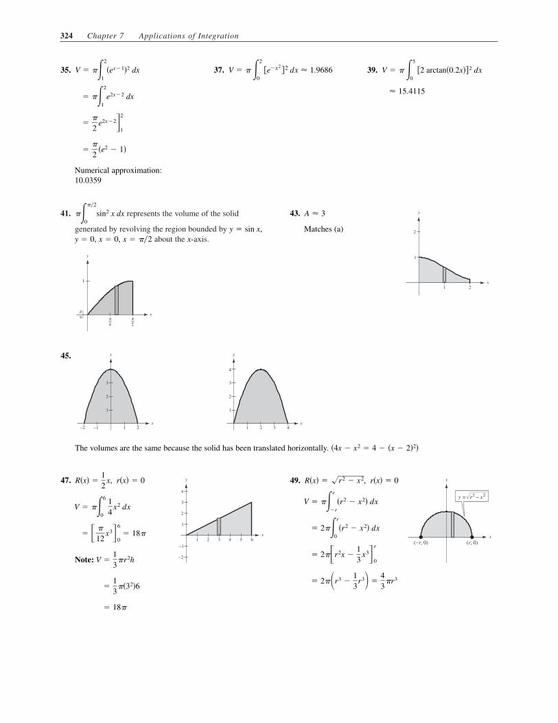
� 2��r3 �13
r3� �43
�r3
� 2��r2x �13
x3�r
0
� 2��r
0�r2 � x2� dx
V � ��r
�r
�r2 � x2� dx
( , 0)−r ( , 0)rx
y = r x−2 2
yr�x� � 0R�x� � �r2 � x2,
35.
Numerical approximation:10.0359
��
2�e2 � 1�
��
2e2x�2�
2
1
� ��2
1e2x�2 dx
V � ��2
1�ex�1�2 dx 37. V � � �2
0 �e�x2 �2 dx 1.9686 39.
15.4115
V � � �5
0 �2 arctan�0.2x��2 dx

Section 7.2 Volume: The Disk Method 325
51.
� �r2h�1 �hH
�h2
3H 2�
� �r2�h �h2
H�
h3
3H 2�
� �r2�y �1H
y2 �1
3H 2 y3�h
0
V � ��h
0 �r�1 �
yH��
2
dy � �r2 �h
0 �1 �
2H
y �1
H 2 y2� dy
−r rx
h
H
yr�y� � 0R�y� � r�1 �yH�,x � r �
rH
y � r �1 �yH�,
53. V � ��2
0 � 1
8 x2�2 � x�2
dx ��
64 �2
0 x4�2 � x� dx �
�
64�2x5
5�
x6
6 �2
0�
�
30
55. (a)
� 60�
�18�
25 �25x �x3
3 �5
0
�18�
25 �5
0�25 � x2� dx
x−6 − 4 −2 2 4 6
− 4
−2
2
4
6
8
y V �9�
25 �5
�5�25 � x2� dx
r�x� � 0R�x� �35�25 � x2, (b)
� 50�
�25�
9 �9y �y3
3 �3
0
x
2
2
4
4
6
6
y V �25�
9 �3
0�9 � y2� dy
x ≥ 0r�y� � 0,R�y� �53�9 � y2,
57. Total volume:
Volume of water in the tank:
When the tank is one-fourth of its capacity:
Depth:
When the tank is three-fourths of its capacity the depth is 100 � 32.64 � 67.36 feet.
�17.36 � ��50� � 32.64 feet
y0 �17.36
y03 � 7500y0 � 125,000 � 0
125,000 � 7500y0 � y03 � 250,000
14 �
500,000�
3 � � ��2500y0 �y0
3
3�
250,0003 �
� ��2500y0 �y0
3
3�
250,0003 �
� ��2500y �y3
3 �y0
�50
��y0
�50��2500 � y2 �2 dy � ��y0
�50�2500 � y2� dy x
−60
−60
−40
−20
20
20
40
40
60
60
yV �4� �50�3
3�
500,000�
3 ft3

326 Chapter 7 Applications of Integration
59. (a) (ii)
is the volume of a right circularcylinder with radius r and height h.
x
( , )h r
y r=y
��h
0 r2 dx (b) (iv)
is the volume of an ellipsoid withaxes and
(0, )a
( , 0)−b ( , 0)bx
y a= 1 −b2x2
y
2b.2a
��b
�b
�a�1 �x2
b2 �2
dx (c) (iii)
is the volume of a sphere withradius r.
x
( , 0)−r ( , 0)r
y = r x−2 2
y
��r
�r��r2 � x2 �2 dx
(d) (i)
is the volume of a right circular cone with the radiusof the base as r and height h.
x
( , )h r
y = xrh
y
��h
0 �rx
h �2
dx (e) (v)
is the volume of a torus with the radius of its circularcross section as r and the distance from the axis of thetorus to the center of its cross section as R.
x
R
R + r x−2 2
R r x− −2 2
− r r
y
��r
�r��R � �r2 � x2 �2
� �R � �r2 � x2 �2� dx
61.
Base of cross section
(a)
2 + x x− 2
2 + x x− 2
� �4x � 2x2 � x3 �12
x4 �15
x5�2
�1�
8110
V � �2
�1�4 � 4x � 3x2 � 2x3 � x4� dx
� 4 � 4x � 3x2 � 2x3 � x4
A�x� � b2 � �2 � x � x2�2
� �x � 1� � �x2 � 1� � 2 � x � x2
x2 3 4
2
3
4
y
(b)
2 + x x− 2
1
V � �2
�1 �2 � x � x2� dx � �2x �
x2
2�
x3
3 �2
�1�
92
A�x� � bh � �2 � x � x2�1

Section 7.2 Volume: The Disk Method 327
63.
Base of cross section
(a)
(c)
1 − y31 − y3
1 − y3
V ��34
�1
0�1 � 3�y �2 dy �
�34 � 1
10� ��340
��34
�1 � 3�y �2
A�y� �12
bh �12
�1 � 3�y ���32 � �1 � 3�y �
� �y �32
y43 �35
y53�1
0�
110
� �1
0�1 � 2y13 � y 23� dy
V � �1
0�1 � 3�y �2 dy
1 − y3
1 − y3
A�y� � b2 � �1 � 3�y �2
� 1 � 3�y
x1
1
14
14
12
12
34
34
y
(b)
(d)
a
b
1 − y3
V ��
2 �1
0�1 � 3�y �2 dy �
�
2 � 110� �
�
20
��
2�1 � 3�y �2 A�y� �
12
�ab ��
2�2��1 � 3�y �1 � 3�y
2
1 − y3
V �18
� �1
0 �1 � 3�y �2 dy �
�
8 � 1
10� ��
80
A�y� �12
�r2 �12
� �1 � 3�y2 �2
�18
� �1 � 3�y �2
65.
r
R
RR2 2− r
�43
� �R2 � r2�32
� 2� ��R2 � r2�32 ��R2 � r2�32
3 �
� 2� ��R2 � r2�x �x3
3 ��R 2 �r2
0
� 2� ��R2 �r2
0 �R2 � r2 � x2� dx
V � � ��R2 �r2
��R2 �r2
���R2 � x2 �2� r2 � dx 67. V � ��1
0y2 dy � �
y3
3 �1
0�
�
3

328 Chapter 7 Applications of Integration
69.
�2�
15
� ��13
�15�
� ��x3
3�
x5
5 �1
0
V � ��1
0�x2 � x 4� dx 71.
��
2
� ��1 �12�
� ��y �y 2
2 �1
0
V � ��1
0�1 � y� dy 73.
��
6
� ��12
�13�
� ��y2
2�
y3
3 �1
0
V � ��1
0� y � y2� dy
75. (a) When represents a square.
When represents a circle.
(b)
To approximate the volume of the solid, form slices,each of whose area is approximated by the integralabove. Then sum the volumes of these slices.n
n
A � 2 �1
�1 �1 � �x�a�1�a dx � 4 �1
0 �1 � xa�1�a dx
�y� � �1 � �x�a�1�a
x
a = 2
a = 1
−1
−1
1
1
y
a � 2: �x�2 � �y�2 � 1
a � 1: �x� � �y� � 1 77. (a)
(b) is one-quarter of the area of a circle
of radius
V � 8�R�14�r2� � 2�2r2R
r, 14�r2.
�r
0
�r2 � y2 dy
R
x
y
� 8�R�r
0
�r2 � y2 dy
� 2��r
04R�r2 � y2 dy
V � 2��r
0 � R ��r2 � y22
� R ��r2 � y2 2� dy
x � R ± �r2 � y2
�x � R�2 � y2 � r2
Section 7.3 Volume: The Shell Method
1.
� �2� x3
3 �2
0�
16�
3
V � 2��2
0 x�x� dx
h�x� � xp�x� � x, 3.
� �4�
5x5�2�
4
0�
128�
5
� 2��4
0 x3�2 dx
V � 2��4
0 x�x dx
h�x� � �xp�x� � x,
5.
� ��
2x4�
2
0� 8�
V � 2��2
0 x3 dx
x−1 1 2 3
1
2
3
4
yh�x� � x2p�x� � x, 7.
� 4��23
x3 �14
x4�2
0�
16�
3
� 4��2
0 �2x2 � x3� dx
x
1
2
3
4
−1 1 2 3
y
V � 2��2
0 x�4x � 2x2� dx
h�x� � �4x � x2� � x2 � 4x � 2x2p�x� � x,

Section 7.3 Volume: The Shell Method 329
9.
�8�
3
� 2�� x4
4�
43
x3 � 2x2�2
0
V � 2��2
0 �x3 � 4x2 � 4x� dx
� x2 � 4x � 4
h�x� � 4 � �4x � x2�
x
1
2
3
4
−1 1 2 3
yp�x� � x 11.
� 0.986
� �2� �1 �1�e
� ���2�e�x2�2�1
0
� �2� �1
0 e�x2�2 x dx
x1
1
14
14
12
34
34
12
y V � 2��1
0 x� 1
�2�e�x2�2 dx
h�x� �1
�2�e�x2�2p�x� � x,
13.
� 2��y2 �y3
3 �2
0�
8�
3
� 2��2
0 �2y � y2� dy
V � 2��2
0 y�2 � y� dy
h�y� � 2 � yp�y� � y,
15. and if
and if
� 2��y2
2 �1�2
0� 2��y �
y2
2 �1
1�2�
�
4�
�
4�
�
2
V � 2� �1�2
0 y dy � 2� �1
1�2 �1 � y� dy
12
≤ y ≤ 1.h�y� �1y
� 1p�y� � y
x21
1
12
14
12
32
34
y0 ≤ y < 12
.h�y� � 1p�y� � y
17.
�6�
7�27� �
768�
7
� �2��37 y7�3�
8
0
� 2��8
0y 4�3 dy
V � 2��8
0y 3�y dy
x−2 2 4 6
2
4
6
8
yp�y� � y, h�y� � 3�y 19.
� 2��8 �163 � �
16�
3
� 2��2y2 �23
y3�2
0
� 2��2
0�4y � 2y2� dy
x
y
−1 1 2 3 4
−1
1
2
3
4
(2, 2)
V � 2��2
0y�4 � 2y� dy
p�y� � y, h�y� � �4 � y� � �y� � 4 � 2y
21.
� 4��x 4
4� 2x3 � 4x2�
2
0� 16�
� 2� �2��2
0�x3 � 6x2 � 8x� dx
V � 2��2
0�4 � x��4x � 2x2� dx
x
1
2
3
4
1 2 3
yh�x� � 4x � x2 � x2 � 4x � 2x2p�x� � 4 � x,

330 Chapter 7 Applications of Integration
25. The shell method would be easier: shells
Using the disk method: �Note: V �128�
3 �V � ��4
0 �2 � �4 � x �2
� �2 � �4 � x �2 dx
V � 2��4
04 � � y � 2�2 y dy
23.
� 2��x4
4� 3x3 � 10x2�
4
0� 64�
� 2��4
0�x3 � 9x2 � 20x� dx
V � 2��4
0�5 � x��4x � x2� dx
x
−1
1
2
3
4
1 2 3 4
yh�x� � 4x � x2p�x� � 5 � x,
27. (a) Disk
x
2
2
6
4
−1 1 3
8
y
V � ��2
0x6 dx � ��x7
7 �2
0�
128�
7
r�x� � 0 R�x� � x3,
(b) Shell
x
2
2
6
4
−1 1 3
8
y
V � 2��2
0x 4 dx � 2��x5
5 �2
0�
64�
5
h�x� � x3p�x� � x,
(c) Shell
� 2��x 4 �15
x5�2
0�
96�
5
� 2��2
0�4x3 � x4� dx
V � 2��2
0�4 � x�x3 dx
x
2
2
6
4
1 3 4
8
yh�x� � x3p�x� � 4 � x,
29. (a) Shell
(b) Same as part (a) by symmetry
—CONTINUED—
� 2� �a3
2�
4a3
5�
a3
3 � ��a3
15
� 2� � a2
y2 �4a1�2
5y5�2 �
y3
3 �a
0
� 2� �a
0 �ay � 2a1�2y3�2 � y2� dy
V � 2� �a
0 y�a � 2a1�2 y1�2 � y� dy
h�y� � �a1�2 � y1�2�2 p�y� � y,(0, )a
( , 0)ax
y

Section 7.3 Volume: The Shell Method 331
31. Answers will vary. (a) The rectangles would be vertical. (b) The rectangles would be horizontal.
29. —CONTINUED—
(c) Shell
� 2� �a2x �43
a3�2x3�2 �45
a1�2x5�2 �13
x3�a
0�
4� a3
15
� 2��a
0�a2 � 2a3�2x1�2 � 2a1�2x3�2 � x2� dx
V � 2��a
0�a � x��a1�2 � x1�2�2 dx
h�x� � �a1�2 � x1�2�2 p�x� � a � x,(0, )a
( , 0)ax
y
33.
This integral represents the volume of the solid generated by revolving the region bounded byand about the x-axis by using the disk method.
represents this same volume by using the shell method.
Disk method
x
4
3
2
1
−153 421
y
2��2
0y 5 � �y2 � 1� dy
x � 5y � 0,y � �x � 1,
��5
1�x � 1� dx � ��5
1 ��x � 1 �2 dx
35. (a)
(b)
V � 2� �1
0 x�1 � x4�3�3�4 dx � 1.5056
y � �1 � x 4�3�3�4
y � 0x � 0,x 4�3 � y 4�3 � 1,
y x )= (1 − 4/3 3/4
−0.25
−0.25 1.5
1.5 37. (a)
(b) V � 2� �6
2 x 3��x � 2�2�x � 6�2 dx � 187.249
−1
−1
7
y x x= ( 2) ( 6)− −3 2 2
7
39.
Matches (d)
x1 2
1
2
yVolume � 7.5
x � 2x � 0,y � 0,y � 2e�x,

332 Chapter 7 Applications of Integration
41.
Now find such that:
(Quadratic Formula)
Take since the other root is too large.
Diameter: 2�4 � 2�3 � 1.464
x0 � �4 � 2�3 � 0.73205,
x02 � 4 ± 2�3
x04 � 8x0
2 � 4 � 0
1 � 2x02 �
14
x04
1 � 2 �x2 �18
x 4�x0
0
� � 2� �x0
0 �2x �
12
x3 dx
x2
2
1
1
y
x0
V � 2��2
0x�2 �
12
x2 dx � 2��2
0 �2x �
12
x3 dx � 2��x2 �18
x 4�2
0� 4� �total volume�
h�x� � 2 �12
x2p�x� � x,
43.
� 4� 2 � �2� �23 �1 � x2�3�2�
1
�1� 4� 2
� 8� ��
2 � 2��1
�1x�1 � x2�1�2��2� dx
� 8��1
�1
�1 � x2 dx � 4��1
�1x�1 � x2 dx
V � 4��1
�1�2 � x��1 � x2 dx
45. (a)
Hence, �x sin x dx � sin x � x cos x � C.
ddx
sin x � x cos x � C � cos x � x sin x � cos x � x sin x
(b) (i)
x
y
−1.0
−
0.5
1.0
3 4π
2π π
4π
4π
� 2� �1 � 0� � 0 � 2�
� 2��sin x � x cos x���2
0
V � 2����2
0x sin x dx
p�x� � x, h�x� � sin x (ii)
� 6� � � 6� 2
� 6��sin x � x cos x��
0
� 6���
0x sin x dx
x
y
− 5 4π
2π π
4π
−1
−2
1
2
V � 2���
0x�3 sin x� dx
p�x� � x, h�x� � 2 sin x � ��sin x� � 3 sin x

Section 7.3 Volume: The Shell Method 333
47.
(a) Plane region bounded by
(b) Revolved about the axis
Other answers possible
−1 21 3 4
1
2
3
4
x
y
y-
y � x2, y � 0, x � 0, x � 2
2��2
0x3 dx � 2��2
0x�x2� dx 49.
(a) Plane region bounded by
(b) Revolved around line
Other answers possible
x
y
−1−2−3 1 2 3 4 5
1
2
3
4
5
6
−2
x = 6 − y
y � �2
x � �6 � y, x � 0, y � 0
2��6
0� y � 2��6 � y dy
51. Disk Method
� ��r2y �y3
3 �r
r�h�
13
�h2�3r � h�
V � � �r
r�h
�r2 � y2� dy
r�y� � 0
xr−r
r
y R�y� � �r2 � y2
53. (a)
(b)
limn→�
�abn�b � �
limn→�
R1�n� � limn→�
n
n � 1� 1
R1�n� �abn�1n��n � 1�
�abn�b �n
n � 1
� abn�1�1 �1
n � 1 � abn�1� nn � 1
� abn�1 � abn�1
n � 1
� �abnx � axn�1
n � 1�b
0
Area region � �b
0abn � axn dx (c) Disk Method:
(d)
(e) As the graph approaches the line x � 1.n →�,
limn→�
��b2��abn� � �
limn→�
R2�n� � limn→�
� nn � 2 � 1
R2�n� ��abn�2n��n � 2�
��b2��abn� � � nn � 2
� 2�a�bn�2
2�
bn�2
n � 2� � �abn�2� nn � 2
� 2�a�bn
2x2 �
xn�2
n � 2�b
0
� 2�a�b
0�xbn � xn�1� dx
V � 2��b
0x�abn � axn� dx
55. (a)
—CONTINUED—
�20�
35800 � 121,475 cubic feet
�2� �40�
3�4� 0 � 4�10��45� � 2�20��40� � 4�30��20� � 0
V � 2� �4
0 x f �x� dx
334 Chapter 7 Applications of Integration
57.
(a)
� �� x 4
4�
8x3
3� 8x2�
4
0�
64�
3
� ��4
0�x3 � 8x2 � 16x� dx
V � ��4
0x�4 � x�2 dx
y2 � ��x�4 � x�2 � ��4 � x��x
y1 � �x�4 � x�2 � �4 � x��x
1 2 3 4 5 6−1
−2
−3
−4
1
2
3
4
x
y y2 � x�4 � x�2, 0 ≤ x ≤ 4
(b)
� 4��85
x5�2 �27
x7�2�4
0�
2048�
35
� 4��4
0�4x3�2 � x5�2� dx
V � 4��4
0x�4 � x��x dx (c)
� 4��323
x3�2 �165
x5�2 �27
x7�2�4
0�
8192�
105
� 4��4
0�16�x � 8x3�2 � x5�2� dx
V � 4��4
0�4 � x��4 � x��x dx
55. —CONTINUED—
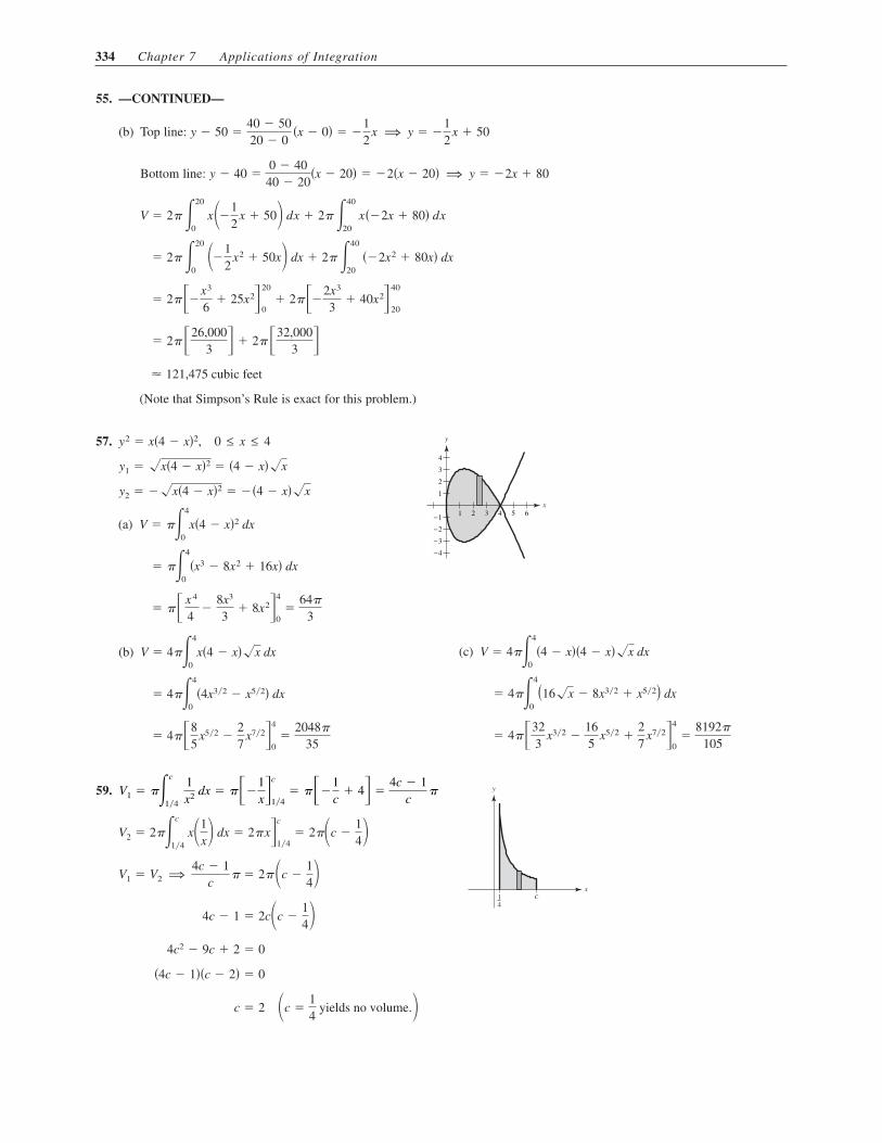
(b) Top line:
Bottom line:
(Note that Simpson’s Rule is exact for this problem.)
� 121,475 cubic feet
� 2� �26,0003 � � 2� �32,000
3 �
� 2���x3
6� 25x2�
20
0� 2���2x3
3� 40x2�
40
20
� 2� �20
0 ��1
2x2 � 50x dx � 2� �40
20 ��2x2 � 80x� dx
V � 2� �20
0 x��1
2x � 50 dx � 2� �40
20 x��2x � 80� dx
y � 40 �0 � 40
40 � 20�x � 20� � �2�x � 20� ⇒ y � �2x � 80
y � 50 �40 � 5020 � 0
�x � 0� � �12
x ⇒ y � �12
x � 50
59.
c � 2 �c �14
yields no volume. �4c � 1��c � 2� � 0
4c2 � 9c � 2 � 0
4c � 1 � 2c�c �14
V1 � V2 ⇒ 4c � 1c
� � 2��c �14
V2 � 2��c
1�4 x�1
x dx � 2�x�c
1�4� 2��c �
14
c14
x
y V1 � ��c
1�4
1x2 dx � ���
1x�
c
1�4� ���
1c
� 4� �4c � 1
c�
Section 7.4 Arc Length and Surfaces of Revolution
1.
(a)
(b)
� �135
x�5
0� 13
s � �5
0�1 � � 12
5 �2
dx
y� �125
y �125
x
� 13
d � ��5 � 0�2 � �12 � 0�2
�0, 0�, �5, 12� 3.
�23
��8 � 1� 1.219
� �23
�1 � x�32�1
0
s � �1
0 �1 � x dx
y� � x12, 0 ≤ x ≤ 1
y �23
x32 � 1 5.
� 5�5 � 2�2 8.352
�32 �
23
�x23 � 1�32�8
1
�32
�8
1 �x23 � 1� 2
3x13� dx
� �8
1 �x23 � 1
x23 dx
s � �8
1 �1 � � 1
x13�2
dx
y� �1
x13, 1 ≤ x ≤ 8
y �32
x23
7.
� � 110
x5 �1
6x3�2
1�
779240
3.2458
� �2
1 � 1
2x4 �
12x4� dx
� �2
1 ��1
2x4 �
12x4�
2
dx
s � �b
a
�1 � �y��2 dx
1 � �y��2 � �12
x4 �1
2x4�2
, 1 ≤ x ≤ 2
y� �12
x4 �1
2x4
y �x5
10�
16x3 9.
� ln��2 � 1� � ln��2 � 1� 1.763
� �ln�csc x � cot x��3�4
�4
s � �3�4
�4 csc x dx
1 � �y� �2 � 1 � cot2 x � csc2 x
y� �1
sin x cos x � cot x
y � ln�sin x�, ��
4,
3�
4 �
11.
�12 �ex � e�x�
2
0�
12 �e2 �
1e2� 3.627
�12
�2
0 �ex � e�x� dx
s � �2
0��1
2�ex � e�x��
2
dx
1 � �y� �2 � �12
�ex � e�x��2
, �0, 2
y� �12
�ex � e�x�, �0, 2
y �12
�ex � e�x� 13.
� �y3
3� y�
4
0�
643
� 4 �763
� �4
0�y2 � 1� dy
� �4
0
�y 4 � 2y2 � 1 dy
s � �4
0
�1 � y2�y2 � 2� dy
dxdy
� y�y2 � 2�12
x �13
�y2 � 2�32, 0 ≤ y ≤ 4
Section 7.4 Arc Length and Surfaces of Revolution 335

336 Chapter 7 Applications of Integration
19. (a)
−0.5
2
3 �2�
2�−
y � sin x, 0 ≤ x ≤ � (b)
L � ��
0
�1 � cos2 x dx
1 � �y� �2 � 1 � cos2 x
y� � cos x (c) L 3.820
21. (a)
−1
−1
3
3
1 ≥ x ≥ e�2 0.135
y � �ln x
0 ≤ y ≤ 2x � e�y, (b)
L � �1
e�2�1 �
1x2 dx
1 � �y� �2 � 1 �1x2
y� � �1x
(c) L 2.221
Alternatively, you can do all the computations with respect to y.
(a) 0 ≤ y ≤ 2x � e�y, (b)
L � �2
0
�1 � e�2y dy
1 � �dxdy�
2
� 1 � e�2y
dxdy
� �e�y (c) L 2.221
23. (a)
−3
1.5−0.5
3
y � 2 arctan x, 0 ≤ x ≤ 1 (b)
L � �1
0�1 �
4�1 � x2�2 dx
y� �2
1 � x2 (c) L 1.871
15. (a)
−1
−1
3
5
y � 4 � x2, 0 ≤ x ≤ 2 (b)
L � �2
0
�1 � 4x2 dx
1 � �y� �2 � 1 � 4x2
y� � �2x (c) L 4.647
17. (a)
−1
−1
4
2
y �1x
, 1 ≤ x ≤ 3 (b)
L � �3
1�1 �
1x4 dx
1 � �y� �2 � 1 �1x4
y� � �1x2 (c) L 2.147

Section 7.4 Arc Length and Surfaces of Revolution 337
25.
Matches (b)
s 5
x
(0, 5)
(2, 1)
−1 1 2 3 4
5
4
3
2
1
5x2 + 1
y =
y�2
0�1 � � d
dx �5
x2 � 1��2
dx
27.
(a)
(b)
(c) (Simpson’s Rule, )
(d) 64.672
n � 10s � �4
0
�1 � �3x2�2 dx � �4
0
�1 � 9x4 dx 64.666
64.525
d � ��1 � 0�2 � �1 � 0�2 � ��2 � 1�2 � �8 � 1�2 � ��3 � 2�2 � �27 � 8�2 � ��4 � 3�2 � �64 � 27�2
d � ��4 � 0�2 � �64 � 0�2 64.125
�0, 4 y � x3,
29. (a)
(c)
Divide into two intervals.
�1
27�4032 � 1332 � 16 10.5131
s1 � s2 �1
27�4032 � 8 � 8 � 1332
� �1
27�8 � 1332� 1.4397
� �1
27�432 � 1332�
� �1
27�9x23 � 4�32�
0
�1
� �1
18�0
�1�9x23 � 4�12� 6
x13� dx
��13 �0
�1
�9x23 � 41
x13 dx, �x0�
s1 � �0
�1�9x23 � 4
9x23 dx��1, 0 :
��1, 8
1 � f ��x�2 � 1 �4
9x23 �9x23 � 4
9x23
f ��x� �23
x�13
10
−2
−2
10
f �x� � x23 (b) No, is not defined.
�127
�4032 � 8� 9.0734
�1
27�4032 � 432�
�1
27�9x23 � 4�32�
8
0
�13�
8
0
�9x23 � 41
x13 dx, �x ≥ 0�
s2 � �8
0�9x23 � 4
9x23 dx�0, 8 :
f ��0�
338 Chapter 7 Applications of Integration
35.
� 2�20� sinh x
20�20
0� 40 sinh�1� 47.008 m
L � �20
�20 cosh
x20
dx � 2�20
0 cosh
x20
dx
1 � �y� �2 � 1 � sinh2 x
20� cosh2
x20
y� � sinh x
20
y � 20 cosh x
20, �20 ≤ x ≤ 20 37.
� 3 arcsin 23
2.1892
� �3 arcsin x3�
2
0� 3�arcsin
23
� arcsin 0�
s � �2
0� 9
9 � x2 dx � �2
0
3�9 � x2
dx
1 � �y� �2 �9
9 � x2
y� ��x
�9 � x2
y � �9 � x2
31. (a)
(b)
(c)
L4 � �4
0�1 �
25256
x3 dx 6.063y4� �5
16x 32,
L3 � �4
0�1 �
x2
4 dx 5.916y3� �
12
x,
L2 � �4
0�1 �
9x16
dx 5.759y2� �34
x12,
L1 � �4
0
�2 dx 5.657y1� � 1,
y1, y2, y3, y4
x−1 1 2 3 4 5
−1
1
2
3
4
5
y
y1
y2
y3
y4
33.
When Thus, the fleeing object has traveledunits when it is caught.
The pursuer has traveled twice the distance that the fleeing object has traveled when it is caught.
� 12 �
23
x32 � 2x12�1
0�
43
� 2�23�
s � �1
0 x � 12x12 dx �
12
�1
0 �x12 � x�12� dx
1 � �y� �2 � 1 ��x � 1�2
4x�
�x � 1�2
4x
y� �13 �
32
x12 �32
x�12� � �12�
x � 1x12
23
y �23.x � 0,
y �13
�x32 � 3x12 � 2
39.
��
9�82�82 � 1� 258.85
� ��
9�1 � x4�32�
3
0
��
6 �3
0 �1 � x4�12�4x3� dx
S � 2� �3
0 x3
3�1 � x4 dx
y� � x2, �0, 3
y �x3
341.
� 2� � x6
72�
x2
6�
18x2�
2
1�
47�
16
� 2� �2
1 �x5
12�
x3
�1
4x3� dx
S � 2� �2
1 �x3
6�
12x��
x2
2�
12x2� dx
1 � �y� �2 � �x2
2�
12x2�
2
, �1, 2
y� �x2
2�
12x2
y �x3
6�
12x

Section 7.4 Arc Length and Surfaces of Revolution 339
47. A rectifiable curve is one that has a finite arc length.
49. The precalculus formula is the surface area formula for the lateral surface of the frustum of a right circular cone.The representative element is
2� f �di ���xi2 � �yi
2 � 2� f �di ��1 � ��yi
�xi�
2
�xi.
51.
� �2��r2 � h2
r �x2
2 ��r
0� �r�r2 � h2
S � 2� �r
0 x�r2 � h2
r2 dx
1 � �y� �2 �r2 � h2
r2
y� �hr
y �hxr
53.
See figure in Exercise 54.
� 6� �3 � �5 � 14.40
� ��6��9 � x2�2
0
� �3� �2
0
�2x�9 � x2
dx
S � 2� �2
0
3x�9 � x2
dx
�1 � �y� �2 �3
�9 � x2
y� ��x
�9 � x2
y � �9 � x2
55.
Amount of glass needed: V ��
27 �0.015
12 � 0.00015 ft3 0.25 in.3
��
3 �13
0 � 1
3� 2x � 9x2� dx �
�
3 � 13
x � x2 � 3x3�13
0�
�
27 ft 2 0.1164 ft2 16.8 in.2
S � 2� �13
0 � 1
3x12 � x32�� 1
36�x�12 � 9x12�2 dx �
2�
6 �13
0 �1
3x12 � x32��x�12 � 9x12� dx
1 � �y� �2 � 1 �1
36�x�1 � 18 � 81x� �
136
�x�12 � 9x12�2
y� �16
x�12 �32
x12 �16
�x�12 � 9x12�
y �13
x12 � x32
43.
��
27�145�145 � 10�10 � 199.48
� � �
27�9x43 � 1�32�
8
1
��
18 �8
1 �9x43 � 1�12�12x13� dx
�2�
3 �8
1 x13�9x43 � 1 dx
S � 2� �8
1 x�1 �
19x43 dx
y� �1
3x23, �1, 8
y � 3�x � 2 45.
14.4236
S � 2� ��
0 sin x�1 � cos2 x dx
y� � cos x, �0, �
y � sin x
340 Chapter 7 Applications of Integration
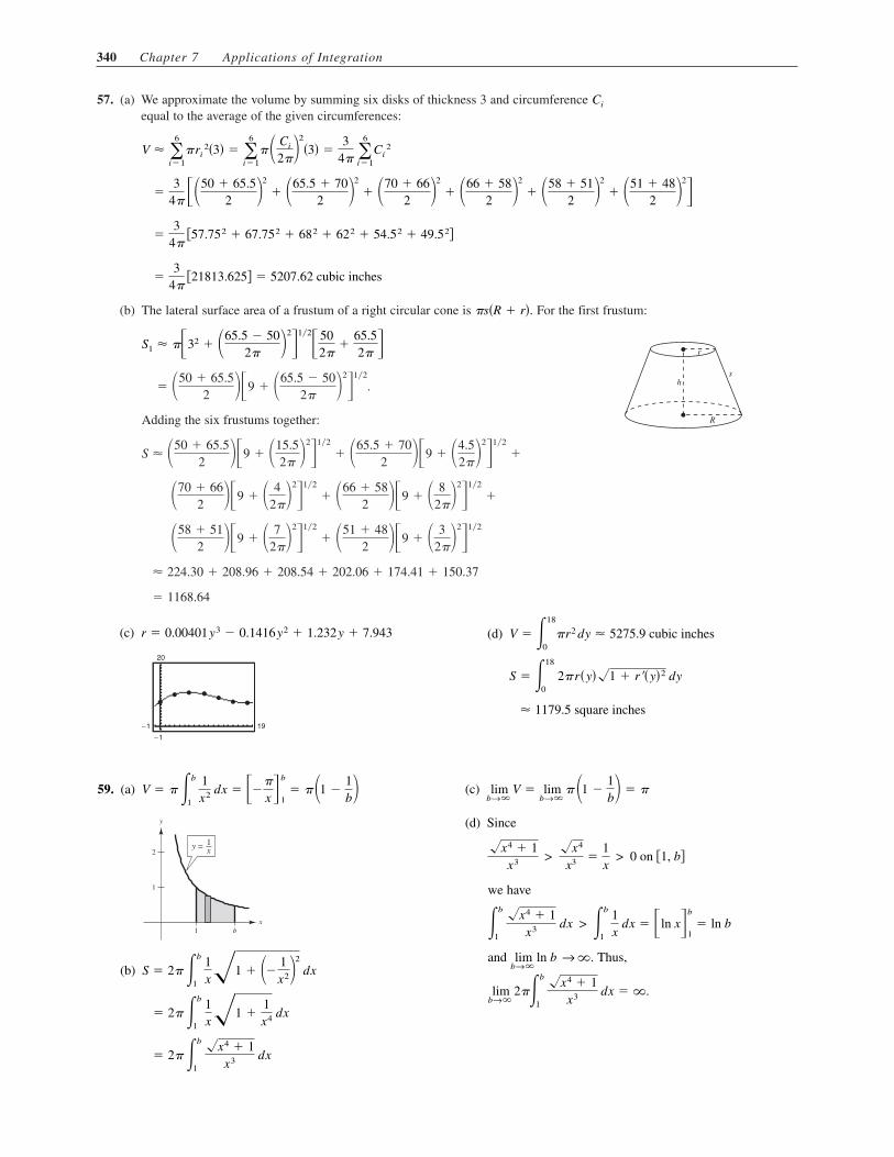
57. (a) We approximate the volume by summing six disks of thickness 3 and circumference equal to the average of the given circumferences:
(b) The lateral surface area of a frustum of a right circular cone is For the first frustum:
Adding the six frustums together:
� 1168.64
224.30 � 208.96 � 208.54 � 202.06 � 174.41 � 150.37
�58 � 512 ��9 � � 7
2��2
�12
� �51 � 482 ��9 � � 3
2��2
�12
�70 � 662 ��9 � � 4
2��2
�12
� �66 � 582 ��9 � � 8
2��2
�12
�
S �50 � 65.52 ��9 � �15.5
2� �2
�12
� �65.5 � 702 ��9 � �4.5
2��2
�12
�
� �50 � 65.52 ��9 � �65.5 � 50
2� �2
�12
.
r
R
sh
S1 ��32 � �65.5 � 502� �
2
�12
� 502�
�65.52� �
�s�R � r�.
�3
4��21813.625 � 5207.62 cubic inches
�3
4��57.752 � 67.752 � 682 � 622 � 54.52 � 49.52
�3
4� ��50 � 65.52 �
2
� �65.5 � 702 �
2
� �70 � 662 �
2
� �66 � 582 �
2
� �58 � 512 �
2
� �51 � 482 �
2
�
V �6
i�1� ri
2�3� � �6
i�1�� Ci
2��2
�3� �3
4� �
6
i�1Ci
2
Ci
(c)
−1
−1 19
20
r � 0.00401y3 � 0.1416y2 � 1.232y � 7.943 (d)
1179.5 square inches
S � �18
0 2�r�y��1 � r��y�2 dy
V � �18
0�r2 dy 5275.9 cubic inches
59. (a)
(b)
� 2� �b
1 �x4 � 1
x3 dx
� 2� �b
1 1x�1 �
1x4 dx
S � 2� �b
1 1x�1 � �� 1
x2�2
dx
x1 b
2
1
y = x1
y
V � � �b
1 1x2 dx � ���
x�b
1� ��1 �
1b� (c)
(d) Since
we have
and Thus,
limb→� 2��b
1 �x4 � 1
x3 dx � �.
limb→� ln b → �.
�b
1 �x4 � 1
x3 dx > �b
1 1x dx � �ln x�
b
1� ln b
�x4 � 1x3 >
�x4
x3 �1x > 0 on �1, b
limb→� V � lim
b→� � �1 �1b� � �

Section 7.5 Work 341
63.
[Surface area of portion above the -axis]x
� ��12�
5�4 � x2�3�5�2�
8
0�
192�
5
� 4��8
0 �4 � x2�3�3�2
x1�3 dx
S � 2��8
0�4 � x2�3�3�2� 4
x2�3 dx
1 � �y� �2 � 1 �4 � x2�3
x2�3 �4
x2�3
y� �32
�4 � x2�3�1�2��23
x�1�3 ���4 � x2�3�1�2
x1�3
y � �4 � x2�3�3�2, 0 ≤ x ≤ 8
y2�3 � 4 � x2�3
x2�3 � y2�3 � 4 65.
By symmetry,
w−w
h(w, h)
x
y
C � 2�w
0 �1 �
4h2
w 4 x2 dx.
h � kw2 ⇒ k �h
w2 ⇒ 1 � �y� � � 1 �4h2
w 4 x2
1 � �y� �2 � 1 � 4k2x2
y � kx2, y� � 2kx
67. Let be the point on the graph of where the tangent linemakes an angle of with the axis.
L � �4�9
0�1 �
94 x dx �
827�2�2 � 1�
x0 �49
y� �32 x1�2 � 1
y � x3�2
x-45�
45�
(x0 , y0)
(0, 0)
y2 = x3
x
yy2 � x3�x0, y0�
61. Individual project
Section 7.5 Work
1.
� 1000 ft � lb
W � Fd � �100��10� 3.
� 448 joules (newton-meters)
W � Fd � �112��4�
5. Work equals force times distance, W � FD. 7. Since the work equals the area under the force function,you have �c� < �d� < �a� < �b�.
9.
� 30.625 in. � lb 2.55 ft � lb
�245
8 in. � lb
W � �7
0 54
x dx � �58
x2�7
0
k �54
5 � k�4�
F�x� � kx 11.
� 87.5 joules or Nm
� 8750 n � cm
� �50
20 253
x dx �25x2
6 �50
20
W � �50
20 F�x� dx
250 � k�30� ⇒ k �253
F�x� � kx
342 Chapter 7 Applications of Integration
17. Assume that Earth has a radius of 4000 miles.
F�x� �80,000,000
x 2
k � 80,000,000
5 �k
�4000�2
F�x� �kx2 (a)
(b)
1395.3 mi � ton 1.47 1010 ft � ton
W � �4300
4000 80,000,000
x2 dx
487.8 mi � tons 5.15 109 ft � lb
W � �4100
4000 80,000,000
x2 dx � ��80,000,000x �
4100
4000
19. Assume that Earth has a radius of 4000 miles.
F�x� �160,000,000
x2
k � 160,000,000
10 �k
�4000�2
F�x� �kx2 (a)
(b)
3.57 1011 ft � lb
3.38 104 mi � ton
� 33,846.154 mi � ton
W � �26,000
4000 160,000,000
x2 dx � ��160,000,000x �
26,000
4000 �6,153.846 � 40,000
3.10 1011 ft � lb
2.93 104 mi � ton
� 29,333.333 mi � ton
W � �15,000
4000 160,000,000
x2 dx � ��160,000,000x �
15,000
4000 �10,666.667 � 40,000
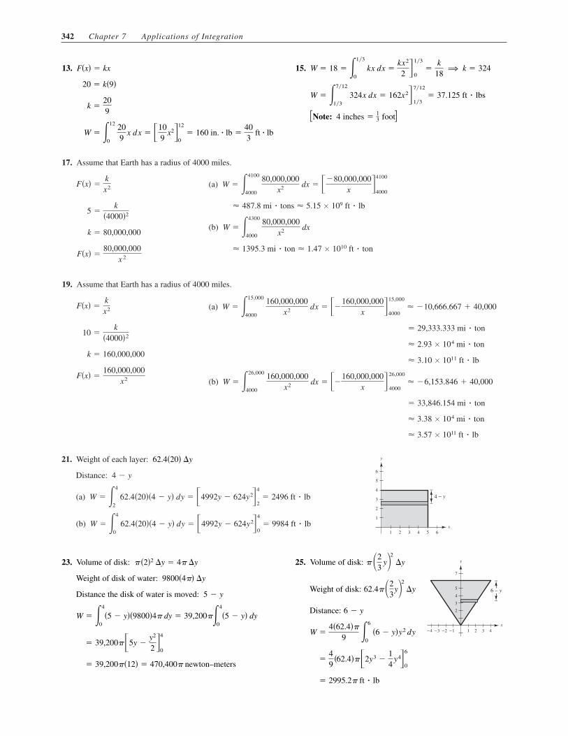
21. Weight of each layer:
Distance:
(a)
(b) W � �4
0 62.4�20��4 � y� dy � �4992y � 624y2�
4
0� 9984 ft � lb
W � �4
2 62.4�20��4 � y� dy � �4992y � 624y2�
4
2� 2496 ft � lb
4 � y
x1 2 3 4 5 6
6
5
4
3
2
1
4 − y
y62.4�20� y
13.
W � �12
0 209
x dx � �109
x2�12
0� 160 in. � lb �
403
ft � lb
k �209
20 � k�9�
F�x� � kx 15.
Note: 4 inches foot��13�
W � �7�12
1�3 324x dx � 162x2�
7�12
1�3� 37.125 ft � lbs
W � 18 � �1�3
0 kx dx �
kx2
2 �1�3
0�
k18
⇒ k � 324
23. Volume of disk:
Weight of disk of water:
Distance the disk of water is moved:
� 39,200��12� � 470,400� newton–meters
� 39,200��5y �y2
2 �4
0
W � �4
0�5 � y��9800�4� dy � 39,200��4
0�5 � y� dy
5 � y
9800�4�� y
� �2�2 y � 4� y 25. Volume of disk:
Weight of disk:
Distance:
� 2995.2� ft � lb
�49
�62.4���2y3 �14
y4�6
0
W �4�62.4��
9 �6
0 �6 � y�y2 dy
6 � y
62.4��23
y2
y
x
6 − y
4321−1−2−3−4
7
5
4
3
2
y� �23
y2
y
Section 7.5 Work 343
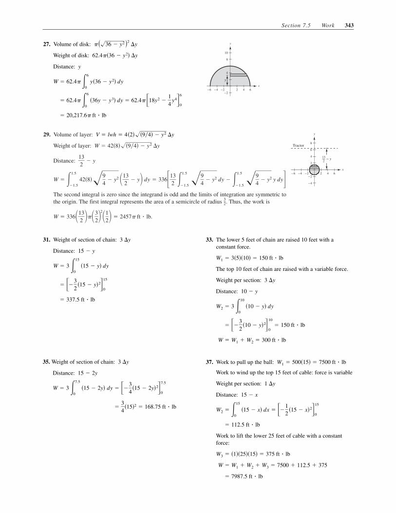
29. Volume of layer:
Weight of layer:
Distance:
The second integral is zero since the integrand is odd and the limits of integration are symmetric to the origin. The first integral represents the area of a semicircle of radius Thus, the work is
W � 336�132 ��3
22
�12 � 2457� ft � lb.
32.
� 336�132
�1.5
�1.5 �9
4� y2 dy � �1.5
�1.5 �9
4� y2 y dy� W � �1.5
�1.5 42�8��9
4� y2 �13
2� y dy
132
� y
W � 42�8���9�4� � y2 y
x
4
2
6
8
642−2−2
−4
−6 −4
132
− y
Tractor
yV � lwh � 4�2���9�4� � y2 y
31. Weight of section of chain:
Distance:
� 337.5 ft � lb
� ��32
�15 � y�2�15
0
W � 3 �15
0 �15 � y� dy
15 � y
3 y 33. The lower 5 feet of chain are raised 10 feet with a constant force.
The top 10 feet of chain are raised with a variable force.
Weight per section:
Distance:
W � W1 � W2 � 300 ft � lb
� ��32
�10 � y�2�10
0� 150 ft � lb
W2 � 3 �10
0 �10 � y� dy
10 � y
3 y
W1 � 3�5��10� � 150 ft � lb
27. Volume of disk:
Weight of disk:
Distance:
� 20,217.6� ft � lb
� 62.4� �6
0 �36y � y3� dy � 62.4� �18y2 �
14
y4�6
0
W � 62.4� �6
0 y�36 � y2� dy
y
62.4��36 � y2� y
x
4
8
10
642−2−2
−6 −4
y
y� ��36 � y2 �2 y
35. Weight of section of chain:
Distance:
�34
�15�2 � 168.75 ft � lb
W � 3 �7.5
0 �15 � 2y� dy � ��3
4�15 � 2y�2�
7.5
0
15 � 2y
3 y 37. Work to pull up the ball:
Work to wind up the top 15 feet of cable: force is variable
Weight per section:
Distance:
Work to lift the lower 25 feet of cable with a constantforce:
� 7987.5 ft � lb
W � W1 � W2 � W3 � 7500 � 112.5 � 375
W3 � �1��25��15� � 375 ft � lb
� 112.5 ft � lb
W2 � �15
0 �15 � x� dx � ��1
2�15 � x�2�
15
0
15 � x
1 y
W1 � 500�15� � 7500 ft � lb

344 Chapter 7 Applications of Integration
43. W � �5
0 1000�1.8 � ln�x � 1�� dx � 3249.44 ft � lb 45. W � �5
0 100x�125 � x3 dx � 10,330.3 ft � lb
Section 7.6 Moments, Centers of Mass, and Centroids
1. x �6��5� � 3�1� � 5�3�
6 � 3 � 5� �
67
3. x �1�7� � 1�8� � 1�12� � 1�15� � 1�18�
1 � 1 � 1 � 1 � 1� 12
5. (a)
(b) x �12��6 � 3� � 1��4 � 3� � 6��2 � 3� � 3�0 � 3� � 11�8 � 3�
12 � 1 � 6 � 3 � 11�
�9933
� �3
x ��7 � 5� � �8 � 5� � �12 � 5� � �15 � 5� � �18 � 5�
5� 17 � 12 � 5
7.
x � 6 feet
125x � 750
50x � 750 � 75x
50x � 75�L � x� � 75�10 � x�
9.
x
2
1
321−1−1
−2
−3
−4
−3 −2
m1
m2
m3
(2, 2)
( 3, 1)−
(1, 4)−
y �x, y � � �109
, �19
y �5�2� � 1�1� � 3��4�
5 � 1 � 3� �
19
x �5�2� � 1��3� � 3�1�
5 � 1 � 3�
109
11.
x642
6
8−2−2
−4
m3m4
m1
m2
m5 (7, 1)(0, 0)
( 2, 3)− −
(5, 5)
( 3, 0)−
y �x, y � � �58
, 1316
y �3��3� � 4�5� � 2�1� � 1�0� � 6�0�
3 � 4 � 2 � 1 � 6�
1316
x �3��2� � 4�5� � 2�7� � 1�0� � 6��3�
3 � 4 � 2 � 1 � 6�
58
39.
� 2000 ln�32 � 810.93 ft � lb
� 2000 ln�V��3
2
W � �3
2 2000
V dV
k � 2000
1000 �k2
p �kV
41.
�3k4
�units of work�
� k2 � x�
1
�2� k�1 �
14
W � �1
�2
k�2 � x�2 dx
F�x� �k
�2 � x�2

Section 7.6 Moments, Centers of Mass, and Centroids 345
13.
�x, y � � �125
, 34
x �My
m�
64�
5 � 316� �
125
My � � �4
0 x�x dx � �
25
x5 2�4
0�
64�
5
y �Mx
m� 4�� 3
16� �34
Mx � � �4
0 �x2
��x � dx � �x2
4 �4
0� 4�
x1 2 3 4
4
3
2
1( , )x y
y m � � �4
0 �x dx � 2�
3x3 2�
4
0�
16�
3
15.
�x, y � � �35
, 1235
x �My
m�
�
20 �12� �
35
My � � �1
0 x�x2 � x3� dx � � �1
0 �x3 � x4� dx � �x4
4�
x5
5 �1
0�
�
20
y �Mx
m�
�
35 �12� �
1235
Mx � � �1
0 �x2 � x3�
2�x2 � x3� dx �
�
2 �1
0 �x4 � x6� dx �
�
2x5
5�
x7
7�1
0�
�
35
x1
1
14
14
12
34
34
12
( , )x y
y
(1, 1)
m � � �1
0 �x2 � x3� dx � �x3
3�
x4
4 �1
0�
�
12
17.
�x, y � � �32
, 225
x �My
m�
27�
4 � 29� �
32
��x4
4� x3�
3
0�
27�
4 My � � �3
0 x ���x2 � 4x � 2� � �x � 2�� dx � � �3
0 ��x3 � 3x2� dx �
y �Mx
m�
99�
5 � 29� �
225
��
2 x5
5� 2x4 �
11x3
3� 6x2�
3
0�
99�
5
��
2 �3
0 ��x2 � 5x � 4���x2 � 3x� dx �
�
2 �3
0 �x4 � 8x3 � 11x2 � 12x� dx
Mx � � �3
0 ��x2 � 4x � 2� � �x � 2�
2 ����x2 � 4x � 2� � �x � 2�� dx
x−1 1 2 3 4
1
2
3
4
5
6
5
( , )x y
y
(3, 5)
m � � �3
0 ���x2 � 4x � 2� � �x � 2�� dx � ��x3
3�
3x2
2 �3
0�
9�
2
346 Chapter 7 Applications of Integration
19.
�x, y � � �5, 107
x �My
m� 96�� 5
96� � 5
My � � �8
0 x�x2 3� dx � �3
8x8 3�
8
0� 96�
y �Mx
m�
192�
7 � 596� �
107
Mx � � �8
0 x2 3
2�x2 3� dx �
�
237
x7 3�8
0�
192�
7
x
2
−2
4
6
4 6 82
( , )x y
y m � � �8
0 x 2 3 dx � �3
5x5 3�
8
0�
96�
5
21.
By symmetry, and
�x, y � � �85
, 0y � 0.Mx
x �My
m�
256�
15 � 332� �
85
My � 2� �2
0 �4 � y2
2 �4 � y2� dy � �16y �83
y3 �y5
5 �2
0�
256�
15x
−2
−1
1
1
32
2
( , )x y
y m � 2� �2
0 �4 � y2� dy � 2�4y �
y3
3�2
0�
32�
3
23.
�x, y � � ��35
, 32
y �Mx
m�
27�
4 � 29� �
32
Mx � � �3
0 y ��2y � y2� � ��y�� dy � � �3
0 �3y2 � y3� dy � �y3 �
y4
4 �3
0�
27�
4
x �My
m� �
27�
10 � 29� � �
35
��
2 �3
0 �y4 � 4y3 � 3y2� dy �
�
2y5
5� y4 � y3�
3
0� �
27�
10
My � � �3
0 ��2y � y2� � ��y��
2��2y � y2� � ��y�� dy �
�
2 �3
0 �y � y2��3y � y2� dy
x
−1
−1−2−3
3
1
1
( , )x y
y
(−3,3) m � � �3
0 ��2y � y2� � ��y�� dy � �3y2
2�
y3
3�3
0�
9�
2
25.
My � �1
0 �x2 � x3� dx � x3
3�
x4
4 �1
0� �1
3�
14 �
112
Mx �12
�1
0 �x2 � x4� dx �
12
x3
3�
x5
5 �1
0�
12 �
13
�15 �
115
A � �1
0 �x � x2� dx � 1
2x2 �
x3
3 �1
0�
16
27.
My � �3
0 �2x2 � 4x� dx � 2x3
3� 2x2�
3
0� 18 � 18 � 36
� 2x3
3� 4x2 � 8x�
3
0� 18 � 36 � 24 � 78
Mx �12
�3
0 �2x � 4�2 dx � �3
0 �2x2 � 8x � 8� dx
A � �3
0 �2x � 4� dx � x2 � 4x�
3
0� 9 � 12 � 21

Section 7.6 Moments, Centers of Mass, and Centroids 347
29.
Therefore, the centroid is �3.0, 126.0�.
y �Mx
m� 126.0
x �My
m� 3.0
My � � �5
0 10x2�125 � x3 dx � �
10�
3 �5
0
�125 � x3 ��3x2� dx �12,500�5�
9� 3105.6�
� 50� �5
0x2�125 � x3� dx �
3,124,375�
24� 130,208�
Mx � � �5
0 �10x�125 � x3
2 �10x�125 � x3 � dx
−50
−1 6
400 m � � �5
0 10x�125 � x3 dx � 1033.0�
31.
by symmetry. Therefore, the centroid is �0, 16.2�.x � 0
y �Mx
m� 16.18
�25�
2 �20
�20 �400 � x2�2 3 dx � 20064.27
Mx � � �20
�20 5 3�400 � x2
2�5 3�400 � x2 � dx
−25
−5
25
50 m � � �20
�20 5 3�400 � x2 dx � 1239.76�
33.
From elementary geometry, is the point of intersection of the medians.�b 3, c 3�
�x, y � � �b3
, c3
�2c
y2
2�
y3
3c�c
0�
c3
�1ac
�c
0 y��2a
cy � 2a dy �
2c �c
0 �y �
y2
c dy
y �1ac
�c
0 y�b � a
cy � a � �b � a
cy � a� dy
�1
2ac 2ab
cy2 �
4ab3c2 y3�
c
0�
12ac �
23
abc �b3
�1
2ac �c
0 4ab
cy �
4abc2 y2� dy
x � � 1ac
12
�c
0 �b � a
cy � a
2
� �b � ac
y � a2
� dy
1A
�1ac
x
( , 0)a( , 0)−a
( , )b c
( , )x y
y = ( + )x acb a+
y = cb a− ( )x a−
y A �12
�2a�c � ac
348 Chapter 7 Applications of Integration
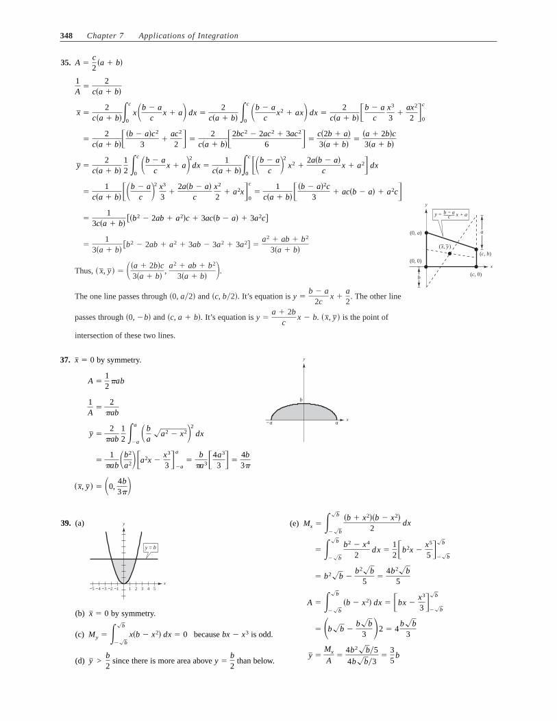
35.
Thus,
The one line passes through and It’s equation is The other line
passes through and It’s equation is is the point of
intersection of these two lines.
�x, y �y �a � 2b
cx � b.�c, a � b�.�0, �b�
y �b � a
2cx �
a2
.�c, b 2�.�0, a 2�
� x, y � � ��a � 2b�c3�a � b� ,
a2 � ab � b2
3�a � b� .
�1
3�a � b� �b2 � 2ab � a2 � 3ab � 3a2 � 3a2� �a2 � ab � b2
3�a � b�
x
( , )x y
cy = b a− x a+
(0, 0)
( , 0)c
( , )c b
(0, )a
b
a
y
�1
3c�a � b� ��b2 � 2ab � a2�c � 3ac�b � a� � 3a2c�
�1
c�a � b� �b � a
c 2
x3
3�
2a�b � a�c
x2
2� a2x�
c
0�
1c�a � b�
�b � a�2c3
� ac�b � a� � a2c�
y �2
c�a � b� 12
�c
0 �b � a
cx � a
2
dx �1
c�a � b��c
0 �b � a
c 2
x2 �2a�b � a�
cx � a2� dx
�2
c�a � b��b � a�c2
3�
ac2
2 � �2
c�a � b�2bc2 � 2ac2 � 3ac2
6 � �c�2b � a�3�a � b� �
�a � 2b�c3�a � b�
2c�a � b�
b � ac
x3
3�
ax2
2 �c
0 x �
2c�a � b��
c
0 x�b � a
cx � a dx �
2c�a � b� �
c
0 �b � a
cx2 � ax dx �
1A
�2
c�a � b�
A �c2
�a � b�
37. by symmetry.
�x, y � � �0, 4b3�
�1
�ab �b2
a2a2x �x3
3 �a
�a�
b�a34a3
3 � �4b3�
y �2
�ab 12
�a
�a
� ba
�a2 � x22
dx
1A
�2
�ab
A �12
�ab
b
−a ax
yx � 0
39. (a)
(b) by symmetry.
(c) because is odd.
(d) since there is more area above than below.y �b2
y > b2
bx � x3My � ��b
��b
x�b � x2� dx � 0
x � 0
−1−2−3−4−5 1 2 3 4 5x
y
y b=
(e)
y �Mx
A�
4b2�b 5
4b�b 3�
35
b
� �b�b �b�b
3 2 � 4b�b
3
A � ��b
��b
�b � x2� dx � bx �x3
3 ��b
��b
� b2�b �b2�b
5�
4b2�b5
� ��b
��b
b2 � x4
2 dx �
12b2x �
x5
5 ��b
��b
Mx � ��b
��b
�b � x2��b � x2�
2 dx
Section 7.6 Moments, Centers of Mass, and Centroids 349
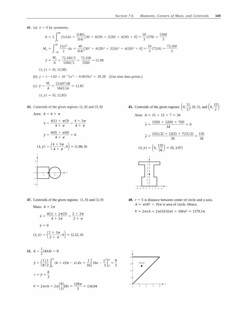
41. (a) by symmetry.
(b) (Use nine data points.)
(c)
�x, y � � �0, 12.85�
y �Mx
A�
23,697.681843.54
� 12.85
y � ��1.02 � 10�5�x 4 � 0.0019x2 � 29.28
�x, y � � �0, 12.98�
y �Mx
A�
72,160 35560 3
�72,1605560
�12.98
Mx � �40
�40 f �x�2
2 dx �
403�4� �302 � 4�29�2 � 2�26�2 � 4�20�2 � 0� �
103
�7216� �72,160
3
A � 2 �40
0 f �x�dx �
2�40�3�4� �30 � 4�29� � 2�26� � 4�20� � 0� �
203
�278� �5560
3
x � 0
43. Centroids of the given regions: and
x1 3
2
1
−1
−2
y
�x, y � � �4 � 3�
4 � �, 0 � �1.88, 0�
y �4�0� � ��0�
4 � �� 0
x �4�1� � ��3�
4 � ��
4 � 3�
4 � �
Area: A � 4 � �
�3, 0��1, 0� 45. Centroids of the given regions: and
x−4 −3 −2 −1 1 2 3 4
7
6
5
4
3
2
1
y
�x, y � � �0, 13534 � �0, 3.97�
y �15�3 2� � 12�5� � 7�15 2�
34�
13534
x �15�0� � 12�0� � 7�0�
34� 0
Area: A � 15 � 12 � 7 � 34
�0, 152 �0,
32, �0, 5�,
47. Centroids of the given regions: and
Mass:
�x, y � � �2 � 3�
2 � �, 0 � �2.22, 0�
y � 0
x �4�1� � 2��3�
4 � 2��
2 � 3�
2 � �
4 � 2�
�3, 0��1, 0� 49. is distance between center of circle and axis.is area of circle. Hence,
V � 2�rA � 2��5��16�� � 160�2 � 1579.14.
A � ��4�2 � 16�y-r � 5
51.
V � 2�rA � 2��83�8� �
128�
3� 134.04
r � y �83
�1
1616x �x3
3�4
0�
83
y � �18
12
�4
0 �4 � x��4 � x� dx
x
1
2
3
4
41 2 3
( , )x y
yA �12
�4��4� � 8
350 Chapter 7 Applications of Integration
Section 7.7 Fluid Pressure and Fluid Force
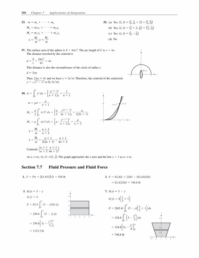
1. F � PA � �62.4�5���3� � 936 lb 3.
� 62.4�2��6� � 748.8 lb
F � 62.4�h � 2��6� � �62.4��h��6�
5.
� 1123.2 lb
� 249.6�3y �y2
2 �3
0
� 249.6 �3
0 �3 � y� dy
F � 62.4 �3
0 �3 � y��4� dy
L�y� � 4
x1 2 3 4
4
3
2
1
yh�y� � 3 � y 7.
� 748.8 lb
� 124.8�3y �y3
9 �3
0
x1−1−2 2
4
2
1
y
� 124.8 �3
0 �3 �
y2
3 dy
F � 2�62.4� �3
0 �3 � y�� y
3� 1 dy
L�y� � 2� y3
� 1h�y� � 3 � y
59.
Centroid:
As The graph approaches the x-axis and the line as n →�.x � 1�x, y � → �1, 14�.n →�,
�n � 1n � 2
, n � 1
4n � 2
y �Mx
m�
n � 12�2n � 1� �
n � 14n � 2
x �My
m�
n � 1n � 2
My � � �1
0 x�xn� dx � �� �
xn�2
n � 2�1
0�
�
n � 2
Mx ��
2 �1
0 �xn�2 dx � ��
2�
x2n�1
2n � 1�1
0�
�
2�2n � 1�
m � �A ��
n � 1
x
1
1
y x= n (1, 1)
yA � �1
0 xn dx � � xn�1
n � 1�1
0�
1n � 1
53.
x �My
m, y �
Mx
m
Mx � m1 y1 � . . . � mn yn
My � m1x1 � . . . � mnxn
m � m1 � . . . � mn 55. (a) Yes.
(b) Yes.
(c) Yes.
(d) No
�x, y� � �56, � 5
18��x, y� � �5
6 � 2, 518� � �17
6 , 518�
�x, y� � �56, 5
18 � 2� � �56, 41
18�
57. The surface area of the sphere is The arc length of C is The distance traveled by the centroid is
This distance is also the circumference of the circle of radius
Thus, and we have Therefore, the centroid of the semicircleis �0, 2r��.y � �r2 � x2
y � 2r�.2�y � 4r
d � 2�y
y.
d �Ss
�4�r2
�r� 4r.
x
(0, )y
−r
r
r
ys � �r.S � 4�r2.
Section 7.7 Fluid Pressure and Fluid Force 351
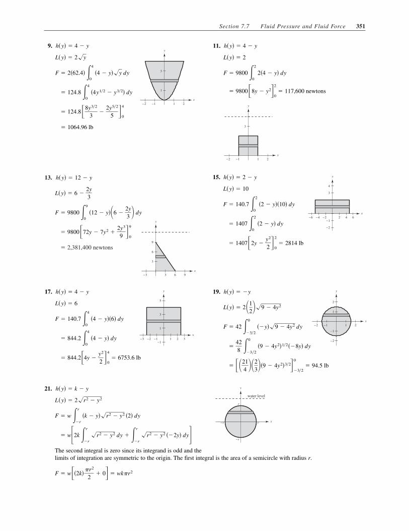
13.
� 2,381,400 newtons
x3−3 6 9
9
6
3
y
� 9800�72y � 7y2 �2y3
9 �9
0
F � 9800 �9
0 �12 � y��6 �
2y3 dy
L�y� � 6 �2y3
h�y� � 12 � y 15.
� 1407�2y �y2
2 �2
0� 2814 lb
� 1407 �2
0 �2 � y� dy
F � 140.7 �2
0 �2 � y��10� dy
L�y� � 10
x
3
4
642−2−1
−2
−6 −4
yh�y� � 2 � y
9.
� 1064.96 lb
� 124.8�8y32
3�
2y52
5 �4
0
� 124.8 �4
0 �4y12 � y32� dy
F � 2�62.4� �4
0 �4 � y��y dy
L�y� � 2�y
x1−1−2 2
3
1
yh�y� � 4 � y 11.
x1−1−2 2
3
y
� 9800�8y � y2�2
0� 117,600 newtons
F � 9800 �2
0 2�4 � y� dy
L�y� � 2
h�y� � 4 � y
17.
� 844.2�4y �y2
2 �4
0� 6753.6 lb
� 844.2 �4
0 �4 � y� dy
F � 140.7 �4
0 �4 � y��6� dy
L�y� � 6
x
3
1
5
321−1−1
−3 −2
yh�y� � 4 � y 19.
� ��214 �2
3�9 � 4y2�32�0
�32� 94.5 lb
�428
�0
�32 �9 � 4y2�12��8y� dy
F � 42 �0
�32 ��y��9 � 4y2 dy
L�y� � 2�12�9 � 4y2
x
2
1
21−2 −1
−2
−1
yh�y� � �y
21.
The second integral is zero since its integrand is odd and the limits of integration are symmetric to the origin. The first integral is the area of a semicircle with radius r.
F � w��2k� �r2
2� 0� � wk�r2
� w�2k �r
�r
�r2 � y2 dy � �r
�r
�r2 � y2 ��2y� dy� F � w �r
�r
�k � y��r2 � y2 �2� dy
L�y� � 2�r2 � y2
x
water level
r
r−r
−r
yh�y� � k � y

352 Chapter 7 Applications of Integration
23.
� wb�ky �y2
2 �h2
�h2� wb�hk� � wkhb
F � w �h2
�h2 �k � y�b dy
L�y� � b
x
2
2
2 2
h
h
b b
water level
−
−
y
k
h�y� � k � y
25. From Exercise 23:
F � 64�15��1��1� � 960 lb
27.
Using Simpson’s Rule with we have:
� 3010.8 lb
F � 62.4�4 � 03�8� �0 � 4�3.5��3� � 2�3��5� � 4�2.5��8� � 2�2��9� � 4�1.5��10� � 2�1��10.25� � 4�0.5��10.5� � 0�
n � 8
F � 62.4 �4
0 �4 � y�L�y� dy
h�y� � 4 � y
29.
� 6448.73 lb
F � 62.4 �4
0 2�12 � y��423 � y23�32 dy
L�y� � 2�423 � y23�32
x−6 −4 −2 2 4 6
10
8
6
4
yh�y� � 12 � y
31. (a) If the fluid force is one-half of 1123.2 lb, and the (b) The pressure increases with increasing depth.height of the water is then
b2 � 4.5 ⇒ b � 2.12 ft.
b2 �b2
2� 2.25
�by �y2
2 �b
0� 2.25
�b
0 �b � y� dy � 2.25
F � 62.4 �b
0 �b � y��4� dy �
12
�1123.2�
L�y� � 4
h�y� � b � y
b,
33. see page 508.F � Fw � w�d
c
h�y�L�y� dy,

1.
3 42
1
5,,125x
y
(1, 0)(5, 0)
(1, 1)
A � �5
1 1x2 dx � ��1
x�5
1�
45
Review Exercises for Chapter 7
3.
��
4� ���
4� ��
2
� �arctan x�1
�12
1
1 1
1
x
,,2
111,,
2
y
(−1, 0) (1, 0)
A � �1
�1
1x2 � 1
dx
5.
�12
� 2�12
x2 �14
x4�1
0
1
1
1
1x
,( )11
0,0(
)1,
)
1(
yA � 2 �1
0 �x � x3� dx 7.
� e2 � 1
� �xe2 � ex�2
0 4
6
3211x
)2,, e(2
)2,, e(0
1),(0
yA � �2
0 �e2 � ex� dx
11.
−4 10
−16
(0, 3)
(8, 3)20
� �8x2 �23
x3�8
0�
5123
� 170.667
� �8
0 �16x � 2x2� dx
A � �8
0 �3 � 8x � x2� � �x2 � 8x � 3� dx9.
4π
2
x
y
21
4π )) ,
215
4π )) , −
�4�2
� 2�2
� � 1�2
�1�2� � �� 1
�2�
1�2�
� ��cos x � sin x�5��4
��4
A � �5��4
��4 �sin x � cos x� dx
13.
−1
(0, 1)
(1, 0)2
2
−1
� �x �43
x3�2 �12
x2�1
0�
16
� 0.1667
� �1
0 �1 � 2x1�2 � x� dx
A � �1
0 �1 � �x�2 dx
y � �1 � �x�215.
�43
� �y2 �13
y3�2
0
� �2
0�2y � y2� dy
A � �2
0 0 � �y2 � 2y� dy
x
3
1
2−2 −1
−1
(0, 2)
(0, 0)
y � �0
�12�x � 1 dx
A � �0
�1 �1 � �x � 1 � � �1 � �x � 1 � dx
x � y2 � 2y ⇒ x � 1 � �y � 1�2 ⇒ y � 1 ± �x � 1
Review Exercises for Chapter 7 353

354 Chapter 7 Applications of Integration
21. (a) Disk
(c) Shell
x2
2
3
4
1
1
3
y
� 2� �2x2 �x3
3 �4
0�
64�
3
� 2� �4
0 �4x � x2� dx
V � 2� �4
0 �4 � x�x dx
x2
2
3 4
4
1
1
3
y
V � � �4
0 x2 dx � ��x3
3 �4
0�
64�
3
(b) Shell
(d) Shell
x2
2
3
4
4 5
5
1
−1
1
3
y
� 2� �3x2 �13
x3�4
0�
160�
3
� 2� �4
0 �6x � x2� dx
V � 2� �4
0 �6 � x�x dx
x2
2
3 4
4
1
1
3
y
V � 2� �4
0 x2 dx � �2�
3x3�
4
0�
128�
3
17.
� �1
0 3y dy � �3
2y2�
1
0�
32
A � �1
0 �y � 2� � �2 � 2y� dy
y � x � 2 ⇒ x � y � 2, y � 1
y � 1 �x2
⇒ x � 2 � 2y
� �2
0 x2
dx � �3
2 �3 � x� dx
A � �2
0 �1 � �1 �
x2�� dx � �3
2 1 � �x � 2� dx
(0, 1) (3, 1)
(2, 0)x
3
3
1
2
y
19. Job 1 is better. The salary for Job 1 is greater than the salary for Job 2 for all the years except the first and 10th years.
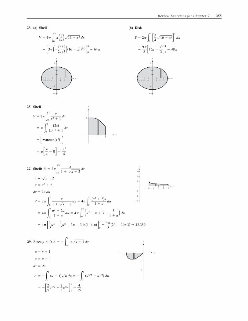
Review Exercises for Chapter 7 355
23. (a) Shell
x2−2
−2
2
3
4
−4
1
1−1−3
y
� �3���12��
23��16 � x2�3�2�
4
0� 64�
V � 4� �4
0 x�3
4��16 � x2 dx
(b) Disk
x2−2
−2
2
3
4
−4
1
1−1−3
y
�9�
8 �16x �x3
3 �4
0� 48�
V � 2� �4
0 �3
4�16 � x2�
2
dx
25. Shell
� ���
4� 0� �
�2
4
� �� arctan�x2��1
0
� � �1
0
�2x��x2�2 � 1
dx
V � 2� �1
0
xx4 � 1
dx
x1
1
y
27. Shell:
� 4� �13
u3 �12
u2 � 3u � 3 ln�1 � u��2
0�
4�
3�20 � 9 ln 3� � 42.359
� 4� �2
0 u3 � 2u1 � u
du � 4� �2
0 �u2 � u � 3 �
31 � u� du
V � 2� �6
2
x
1 � �x � 2 dx � 4� �2
0 �u2 � 2�u
1 � u du
dx � 2u du
x � u2 � 2
u � �x � 2
V � 2��6
2
x
1 � �x � 2 dx
x1
1
2
2
3
3 654
−1
−2
−3
y
29. Since
� ��25
u5�2 �23
u3�2�1
0�
415
A � ��1
0 �u � 1��u du � ��1
0 �u3�2 � u1�2� du
dx � du
x � u � 1
u � x � 1 x
−1
−1
yy ≤ 0, A � ��0
�1 x�x � 1 dx.
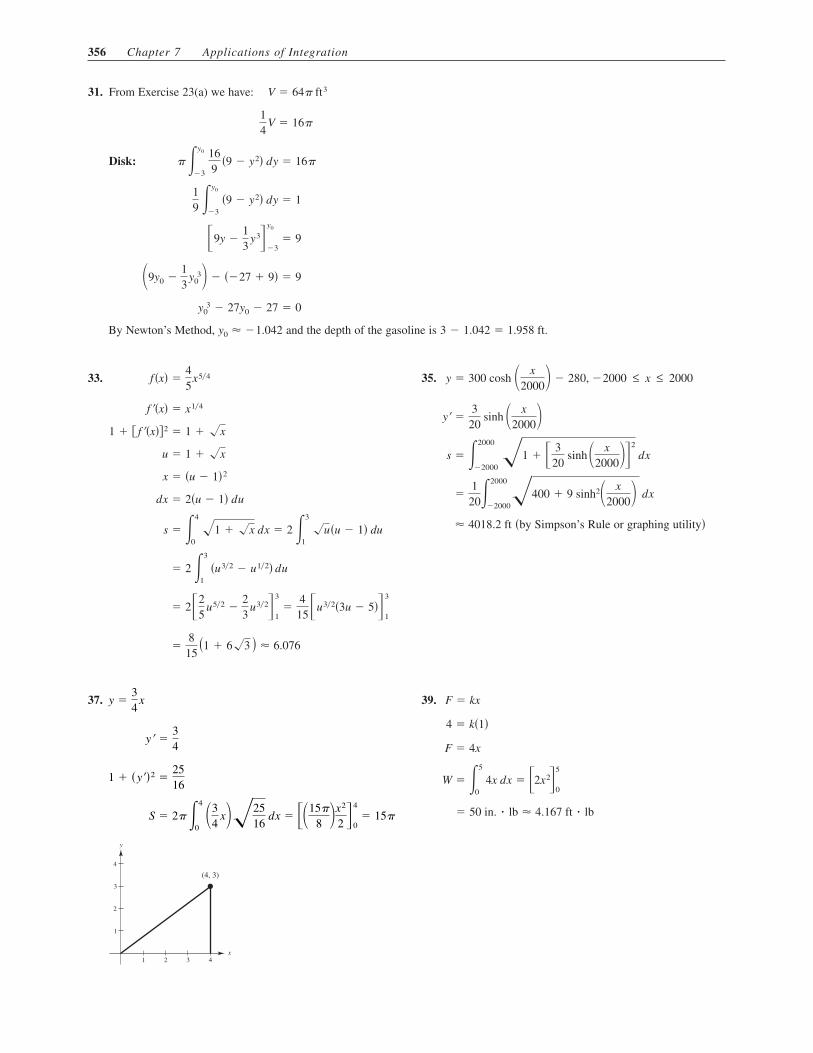
356 Chapter 7 Applications of Integration
31. From Exercise 23(a) we have:
Disk:
By Newton’s Method, and the depth of the gasoline is 3 � 1.042 � 1.958 ft.y0 � �1.042
y03 � 27y0 � 27 � 0
�9y0 �13
y03� � ��27 � 9� � 9
�9y �13
y3�y0
�3� 9
19
�y0
�3 �9 � y2� dy � 1
� �y0
�3 169
�9 � y2� dy � 16�
14
V � 16�
V � 64� ft3
33.
�8
15�1 � 6�3 � � 6.076
� 2�25
u5�2 �23
u3�2�3
1�
415�u3�2�3u � 5��
3
1
� 2 �3
1 �u3�2 � u1�2� du
s � �4
0 �1 � �x dx � 2 �3
1 �u�u � 1� du
dx � 2�u � 1� du
x � �u � 1�2
u � 1 � �x
1 � f��x�2 � 1 � �x
f��x� � x1�4
f �x� �45
x5�4 35.
by Simpson’s Rule or graphing utility�� � 4018.2 ft
�1
20�2000
�2000�400 � 9 sinh2� x
2000� dx
s � �2000
�2000 �1 � � 3
20 sinh� x
2000��2
dx
y� �3
20sinh � x
2000�
y � 300 cosh � x2000� � 280, �2000 ≤ x ≤ 2000
39.
� 50 in. � lb � 4.167 ft � lb
W � �5
0 4x dx � �2x2�
5
0
F � 4x
4 � k�1�
F � kx37.
x2
2
3 4
4
1
1
3
(4, 3)
y
S � 2� �4
0 �3
4x��25
16 dx � ��15�
8 �x2
2 �4
0� 15�
1 � �y��2 �2516
y� �34
y �34
x
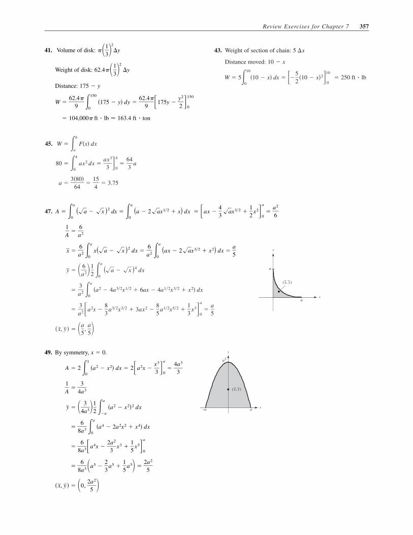
Review Exercises for Chapter 7 357
43. Weight of section of chain:
Distance moved:
W � 5�10
0�10 � x� dx � ��5
2�10 � x�2�10
0� 250 ft � lb
10 � x
5 �x
45.
a �3�80�
64�
154
� 3.75
80 � �4
0 ax2 dx �
ax3
3 �4
0�
643
a
W � �b
a
F�x� dx
47.
�x, y � � �a5
, a5�
�3a2�a2x �
83
a3�2x3�2 � 3ax2 �85
a1�2x5�2 �13
x3�a
0�
a5
�3a2 �a
0 �a2 � 4a3�2x1�2 � 6ax � 4a1�2x3�2 � x2� dx
y � � 6a2� 1
2 �a
0 ��a � �x �4 dx
xa
a
( , )x y
y x �6a2 �a
0 x��a � �x �2 dx �
6a2 �a
0 �ax � 2�ax3�2 � x2� dx �
a5
1A
�6a2
� �ax �43�ax3�2 �
12
x2�a
0�
a2
6A � �a
0 ��a � �x �2 dx � �a
0 �a � 2�ax1�2 � x� dx
41. Volume of disk:
Weight of disk:
Distance:
� 104,000� ft � lb � 163.4 ft � ton
W �62.4�
9 �150
0 �175 � y� dy �
62.4�
9 �175y �y2
2 �150
0
175 � y
62.4��13�
2
�y
��13�
2
�y
49. By symmetry,
�x, y � � �0, 2a2
5 �
�6
8a3 �a5 �23
a5 �15
a5� �2a2
5
�6
8a3�a4x �2a2
3x3 �
15
x5�a
0
�6
8a3 �a
0 �a4 � 2a2x2 � x4� dx
y � � 34a3�1
2 �a
�a
�a2 � x2�2 dx
1A
�3
4a3
A � 2 �1
0 �a2 � x2� dx � 2�a2x �
x3
3 �a
0�
4a3
3
x−a a
a
( , )x y
2
yx � 0.

358 Chapter 7 Applications of Integration
51. by symmetry.
For the trapezoid:
For the semicircle:
Let then and When When
Thus, we have:
The centroid of the blade is �2�9� � 49�3�� � 9� , 0�.
x �180� � 4��4 � 9��
3�
12��9 � �� �
2�9� � 49�3�� � 9�
x�18� � 2��� � 60� �4��4 � 9��
3
� 2����12��
23��4 � u2�3�2�
2
0� 12����2�2
4 � �16�
3� 12�� �
4��4 � 9��3
My � 2� �2
0 �u � 6��4 � u2 du � 2� �2
0 u�4 � u2 du � 12� �2
0 �4 � u2 du
u � 2.x � 8,u � 0.x � 6,dx � du.x � u � 6u � x � 6,
My � � �8
6 x �4 � �x � 6�2 � ���4 � �x � 6�2 � dx � 2� �8
6 x�4 � �x � 6�2 dx
m � �12�����2�2� � 2��
� � �6
0 �1
3x2 � 2x� dx � ��x3
9� x2�
6
0� 60�
My � � �6
0 x��1
6x � 1� � ��1
6x � 1�� dx
m � �4��6� � �1��6�� � 18�
y � 0
(6, 2)
(6, 2)−
x
−4
−1
−2
−3
1
1
2
2
3
3
4
4
5 7
y = x + 116
y
53. Let
x
( , )x yd
c
D
gf
y
� ��Area��depth of centroid�
� ��Area��D � y �
� ���d
c
f �y� � g�y� dy��D ��d
cy f �y� � g�y� dy
�d
c
f �y� � g�y� dy � � ���d
c
D f �y� � g�y� dy � �d
c
y f �y� � g�y� dy� F � � �d
c
�D � y� f �y� � g�y� dy
� � weight per cubic volume.D � surface of liquid;
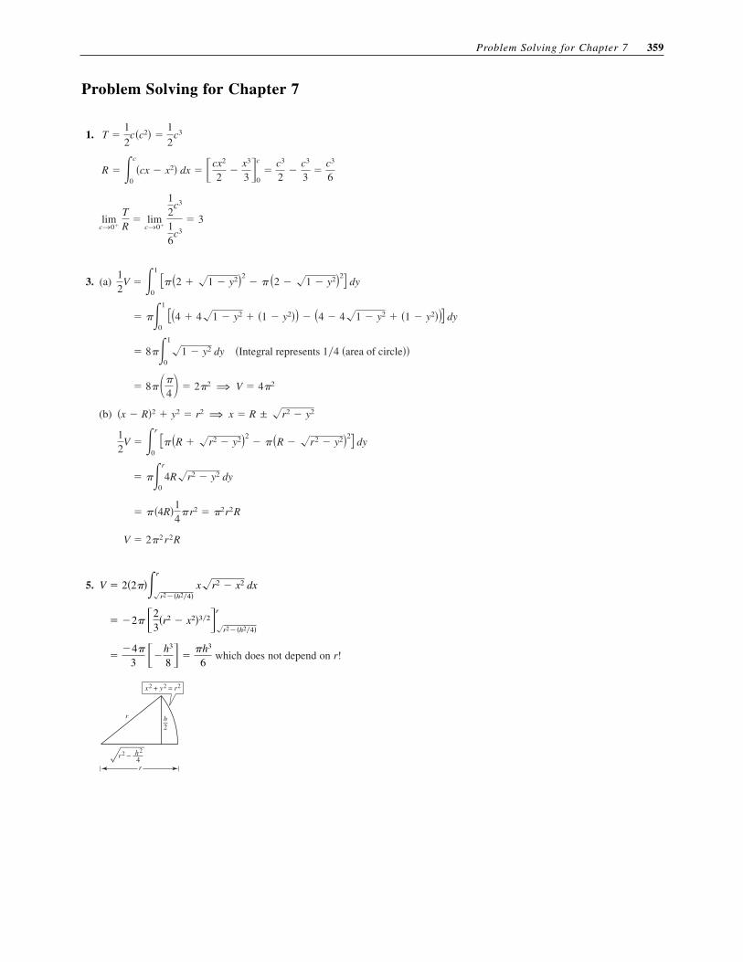
Problem Solving for Chapter 7
1.
limc→0�
TR
� limc→0�
12
c3
16
c3
� 3
R � �c
0�cx � x2� dx � �cx2
2�
x3
3 �c
0�
c3
2�
c3
3�
c3
6
T �1
2c�c2� �
1
2c3
3. (a)
(b)
V � 2�2 r2R
� � �4R�14
�r2 � �2r2R
� ��r
04R�r2 � y2 dy
12
V � �r
0 �� �R � �r2 � y2�2
� � �R � �r2 � y2�2� dy
�x � R�2 � y2 � r2 ⇒ x � R ± �r2 � y2
� 8��
4 � 2�2 ⇒ V � 4�2
� 8��1
0
�1 � y2 dy �Integral represents 1�4 �area of circle��
� ��1
0 ��4 � 4�1 � y2 � �1 � y2�� � �4 � 4�1 � y2 � �1 � y2��� dy
12
V � �1
0 �� �2 � �1 � y2�2
� � �2 � �1 � y2�2� dy
5.
which does not depend on r!
r h2
x2 + y2 = r2
r2 − h2
4r
��4�
3 ��
h3
8 � ��h3
6
� �2� �23
�r2 � x2�3�2�r
�r2��h2�4�
V � 2�2���r
�r2��h2�4� x�r2 � x2 dx
Problem Solving for Chapter 7 359

360 Chapter 7 Applications of Integration
7. (a) Tangent at A:
To find point B:
Tangent at B:
To find point C:
Area of
Area of
Area of �area Sarea R
� 16�S � 16�area of R�
S � �4
�2�12x � 16 � x3� dx � 108
R � �1
�2�x3 � 3x � 2� dx �
274
�x � 2�2�x � 4� � 0 ⇒ C � �4, 64�
x3 � 12x � 16 � 0
x3 � 12x � 16
y � 12x � 16
y � 8 � 12�x � 2�
y � x3, y� � 3x2
�x � 1�2�x � 2� � 0 ⇒ B � ��2, �8�
x3 � 3x � 2 � 0
x3 � 3x � 2
y � 3x � 2
y � 1 � 3�x � 1�
y � x3, y� � 3x2 (b) Tangent at
To find point B:
Tangent at B:
To find point C:
Area of
Area of
Area of S � 16�area of R�
S � �4a
�2a
�12a2x � 16a3 � x3� dx � 108a4
R � �a
�2a
�x3 � 3a2x � 2a3� dx �274
a4
⇒ C � �4a, 64a3�
�x � 2a�2�x � 4a� � 0
x3 � 12a2x � 16a3 � 0
y � 12a2x � 16a3
y � 8a3 � 12a2�x � 2a�
⇒ B � ��2a, �8a3�
�x � a�2�x � 2a� � 0
x3 � 3a2x � 2a3 � 0
y � 3a2x � 2a3
y � a3 � 3a2�x � a�A�a, a3�:
9.
(a)
(b)
(c)
(d)
This is the length of the curve from to x � 2.x � 1y � x3�2
�2227�22 �
1327�13 � 2.0858 s�2� � �2
1�1 �
94
t dt � � 8271 �
94
t3�2
�2
1
s�x� � �x
1�1 � 3
2t1�2
2
dt � �x
1�1 �
94
t dt
�ds�2 � �1 � f��x�2��dx�2 � �1 � dydx
2
��dx�2 � �dx�2 � �dy�2
ds � �1 � f��x�2 dx
s��x� �dsdx
� �1 � f��x�2
s�x� � �x
�
�1 � f��t�2 dt
11. (a) by symmetry
3
2
−1
−2
−3
4 5 632
1
x
y
�x, y� � 127
, 0 x �5�3
35�36�
127
m � 2�6
1
1x3 dx � ��
1x2�
6
1�
3536
My ��6
1x 1
x3 � �1x3 dx ��6
1
2x2 dx � ��2
1x�
6
1�
53
y � 0 (b)
(c) �x, y� � �2, 0�limb→�
x � limb→�
2b
b � 1� 2
�x, y� � 2bb � 1
, 0 x �2�b � 1��b�b2 � 1��b2 �
2bb � 1
My � 2�6
1
1x2 dx �
2�b � 1�b
m � 2�b
1
1x3 dx �
b2 � 1b2

Problem Solving for Chapter 7 361
13. (a)
(b) W � area � 3 � �1 � 1� � 2 �12
� 712
W � area � 2 � 4 � 6 � 12
15. Point of equilibrium:
Consumer surplus
Producer surplus � �80
0�10 � 0.125x� dx � 400
� �80
0��50 � 0.5x� � 10� dx � 1600
�P0, x0� � �10, 80�
x � 80, p � 10
50 � 0.5x � 0.125x
17. We use Exercise 23, Section 7.7, which gives for a rectangle plate.
Wall at shallow end
From Exercise 23:
Wall at deep end
From Exercise 23:
Side wall
From Exercise 23:
Total force: F1 � F2 � 46,592 lb
� 26,624 lb
� 624 �4
0 �8y � y2� dy � 624�4y2 �
y3
3 �4
0
F2 � 62.4 �4
0 �8 � y��10y� dy
F1 � 62.4�2��4��40� � 19,968 lb
5
5
10
10
15
15
20
20
25 40 45x
y = 8x = 40
y = x110
yF � 62.4�4��8��20� � 39,936 lb
F � 62.4�2��4��20� � 9984 lb
F � wkhb