Chapter 6 Vector Fields, Lie Derivatives, Integral …cis610/cis610-15-sl6.pdf · Chapter 6 Vector...
50
Chapter 6 Vector Fields, Lie Derivatives, Integral Curves, Flows Our goal in this chapter is to generalize the concept of a vector field to manifolds, and to promote some standard results about ordinary di↵erential equations to manifolds. 6.1 Tangent and Cotangent Bundles Let M be a C k -manifold (with k ≥ 2). Roughly speaking, a vector field on M is the assignment, p 7! X (p), of a tangent vector X (p) 2 T p (M ), to a point p 2 M . Generally, we would like such assignments to have some smoothness properties when p varies in M , for example, to be C l , for some l related to k . 401
Transcript of Chapter 6 Vector Fields, Lie Derivatives, Integral …cis610/cis610-15-sl6.pdf · Chapter 6 Vector...
Chapter 6
Vector Fields, Lie Derivatives,Integral Curves, Flows
Our goal in this chapter is to generalize the concept of avector field to manifolds, and to promote some standardresults about ordinary di↵erential equations to manifolds.
6.1 Tangent and Cotangent Bundles
LetM be aCk-manifold (with k � 2). Roughly speaking,a vector field on M is the assignment, p 7! X(p), of atangent vector X(p) 2 Tp(M), to a point p 2 M .
Generally, we would like such assignments to have somesmoothness properties when p varies in M , for example,to be Cl, for some l related to k.
401
402 CHAPTER 6. VECTOR FIELDS, INTEGRAL CURVES, FLOWS
Now, if the collection, T (M), of all tangent spaces, Tp(M),was a Cl-manifold, then it would be very easy to definewhat we mean by a Cl-vector field: We would simplyrequire the map, X : M ! T (M), to be Cl.
If M is a Ck-manifold of dimension n, then we can indeedmake T (M) into a Ck�1-manifold of dimension 2n andwe now sketch this construction.
We find it most convenient to use Version 2 of the def-inition of tangent vectors, i.e., as equivalence classes oftriples (U,', x), with x 2 Rn. Recall that (U,', x) and(V, , y) are equivalent i↵
( � '�1)0'(p)
(x) = y.
First, we let T (M) be the disjoint union of the tangentspaces Tp(M), for all p 2 M . Formally,
T (M) = {(p, v) | p 2 M, v 2 Tp(M)}.
There is a natural projection ,
⇡ : T (M) ! M, with ⇡(p, v) = p.
6.1. TANGENT AND COTANGENT BUNDLES 403
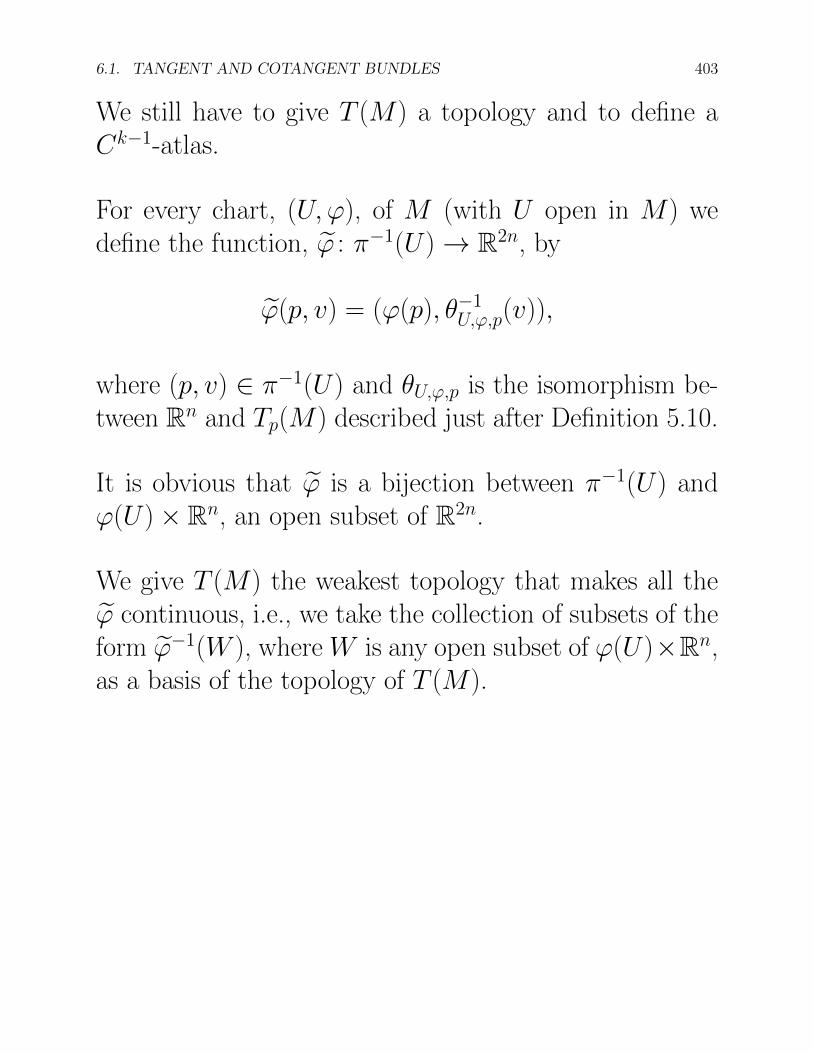
We still have to give T (M) a topology and to define aCk�1-atlas.
For every chart, (U,'), of M (with U open in M) wedefine the function, e' : ⇡�1(U) ! R2n, by
e'(p, v) = ('(p), ✓�1
U,',p(v)),
where (p, v) 2 ⇡�1(U) and ✓U,',p is the isomorphism be-tween Rn and Tp(M) described just after Definition 5.10.
It is obvious that e' is a bijection between ⇡�1(U) and'(U) ⇥ Rn, an open subset of R2n.
We give T (M) the weakest topology that makes all thee' continuous, i.e., we take the collection of subsets of theform e'�1(W ), where W is any open subset of '(U)⇥Rn,as a basis of the topology of T (M).
404 CHAPTER 6. VECTOR FIELDS, INTEGRAL CURVES, FLOWS
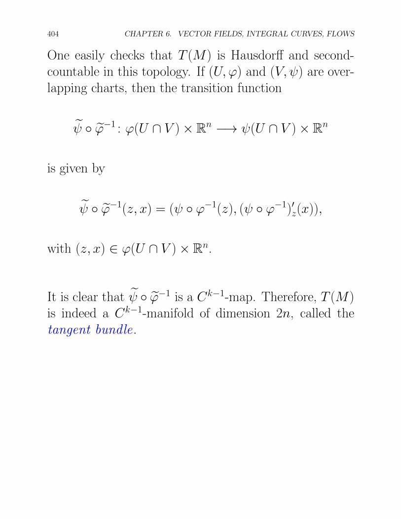
One easily checks that T (M) is Hausdor↵ and second-countable in this topology. If (U,') and (V, ) are over-lapping charts, then the transition function
e � e'�1 : '(U \ V ) ⇥ Rn �! (U \ V ) ⇥ Rn
is given by
e � e'�1(z, x) = ( � '�1(z), ( � '�1)0z(x)),
with (z, x) 2 '(U \ V ) ⇥ Rn.
It is clear that e � e'�1 is a Ck�1-map. Therefore, T (M)is indeed a Ck�1-manifold of dimension 2n, called thetangent bundle .
6.1. TANGENT AND COTANGENT BUNDLES 405
Remark: Even if the manifold M is naturally embed-ded in RN (for some N � n = dim(M)), it is not at allobvious how to view the tangent bundle, T (M), as em-bedded in RN 0
, for some suitable N 0. Hence, we see thatthe definition of an abtract manifold is unavoidable.
A similar construction can be carried out for the cotan-gent bundle.
In this case, we let T ⇤(M) be the disjoint union of thecotangent spaces T ⇤
p (M),
T ⇤(M) = {(p,!) | p 2 M,! 2 T ⇤p (M)}.
We also have a natural projection, ⇡ : T ⇤(M) ! M .
We can define charts as follows:
406 CHAPTER 6. VECTOR FIELDS, INTEGRAL CURVES, FLOWS
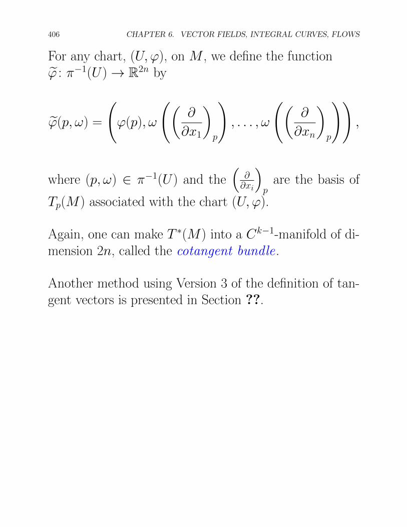
For any chart, (U,'), on M , we define the functione' : ⇡�1(U) ! R2n by
e'(p,!) = '(p),!
✓@
@x1
◆
p
!, . . . ,!
✓@
@xn
◆
p
!!,
where (p,!) 2 ⇡�1(U) and the⇣
@@xi
⌘
pare the basis of
Tp(M) associated with the chart (U,').
Again, one can make T ⇤(M) into a Ck�1-manifold of di-mension 2n, called the cotangent bundle .
Another method using Version 3 of the definition of tan-gent vectors is presented in Section ??.
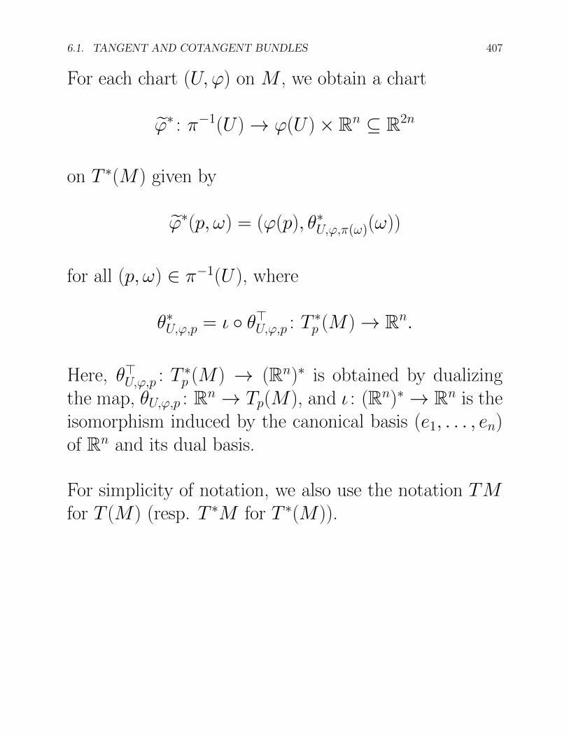
6.1. TANGENT AND COTANGENT BUNDLES 407
For each chart (U,') on M , we obtain a chart
e'⇤ : ⇡�1(U) ! '(U) ⇥ Rn ✓ R2n
on T ⇤(M) given by
e'⇤(p,!) = ('(p), ✓⇤U,',⇡(!)
(!))
for all (p,!) 2 ⇡�1(U), where
✓⇤U,',p = ◆ � ✓>
U,',p : T ⇤p (M) ! Rn.
Here, ✓>U,',p : T ⇤
p (M) ! (Rn)⇤ is obtained by dualizingthe map, ✓U,',p : Rn ! Tp(M), and ◆ : (Rn)⇤ ! Rn is theisomorphism induced by the canonical basis (e
1
, . . . , en)of Rn and its dual basis.
For simplicity of notation, we also use the notation TMfor T (M) (resp. T ⇤M for T ⇤(M)).
408 CHAPTER 6. VECTOR FIELDS, INTEGRAL CURVES, FLOWS
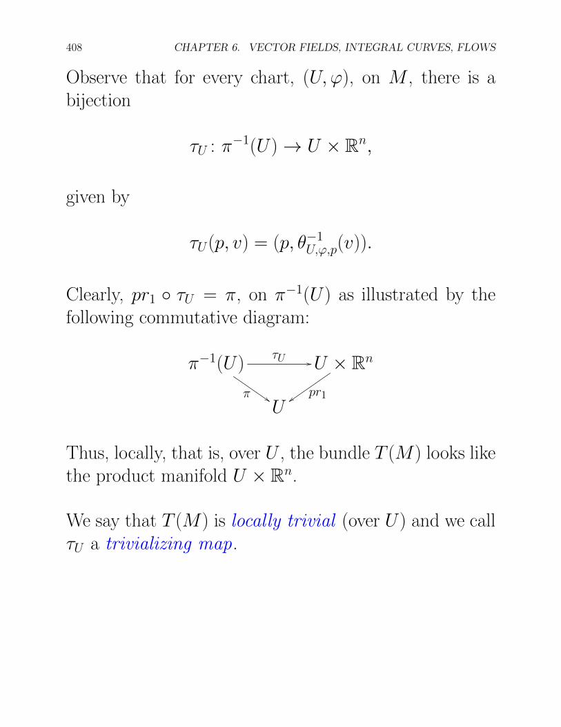
Observe that for every chart, (U,'), on M , there is abijection
⌧U : ⇡�1(U) ! U ⇥ Rn,
given by
⌧U(p, v) = (p, ✓�1
U,',p(v)).
Clearly, pr1
� ⌧U = ⇡, on ⇡�1(U) as illustrated by thefollowing commutative diagram:
⇡�1(U)⌧U //
⇡ $$
U ⇥ Rn
pr1zz
U
Thus, locally, that is, over U , the bundle T (M) looks likethe product manifold U ⇥ Rn.
We say that T (M) is locally trivial (over U) and we call⌧U a trivializing map.

6.1. TANGENT AND COTANGENT BUNDLES 409
For any p 2 M , the vector space⇡�1(p) = {p} ⇥ Tp(M) ⇠= Tp(M) is called thefibre above p.
Observe that the restriction of ⌧U to ⇡�1(p) is an isomor-phism between {p} ⇥ Tp(M) ⇠= Tp(M) and{p} ⇥ Rn ⇠= Rn, for any p 2 M .
Furthermore, for any two overlapping charts (U,') and(V, ), there is a function gUV : U \V ! GL(n,R) suchthat
(⌧U � ⌧�1
V )(p, x) = (p, gUV (p)(x))
for all p 2 U \ V and all x 2 Rn, with gUV (p) given by
gUV (p) = (' � �1)0 (p)
.
Obviously, gUV (p) is a linear isomorphism of Rn for allp 2 U \ V .

410 CHAPTER 6. VECTOR FIELDS, INTEGRAL CURVES, FLOWS
The maps gUV (p) are called the transition functions ofthe tangent bundle.
For example, if M = Sn, the n-sphere in Rn+1, we havetwo charts given by the stereographic projection (UN, �N)from the north pole, and the stereographic projection(US, �S) from the south pole (with UN = Sn � {N}and US = Sn � {S}), and on the overlap, UN \ US =Sn � {N, S}, the transition maps
I = �S � ��1
N = �N � ��1
S
defined on 'N(UN \ US) = 'S(UN \ US) = Rn � {0},are given by
(x1
, . . . , xn) 7! 1Pni=1
x2
i
(x1
, . . . , xn);
that is, the inversion I of center O = (0, . . . , 0) andpower 1.
6.1. TANGENT AND COTANGENT BUNDLES 411
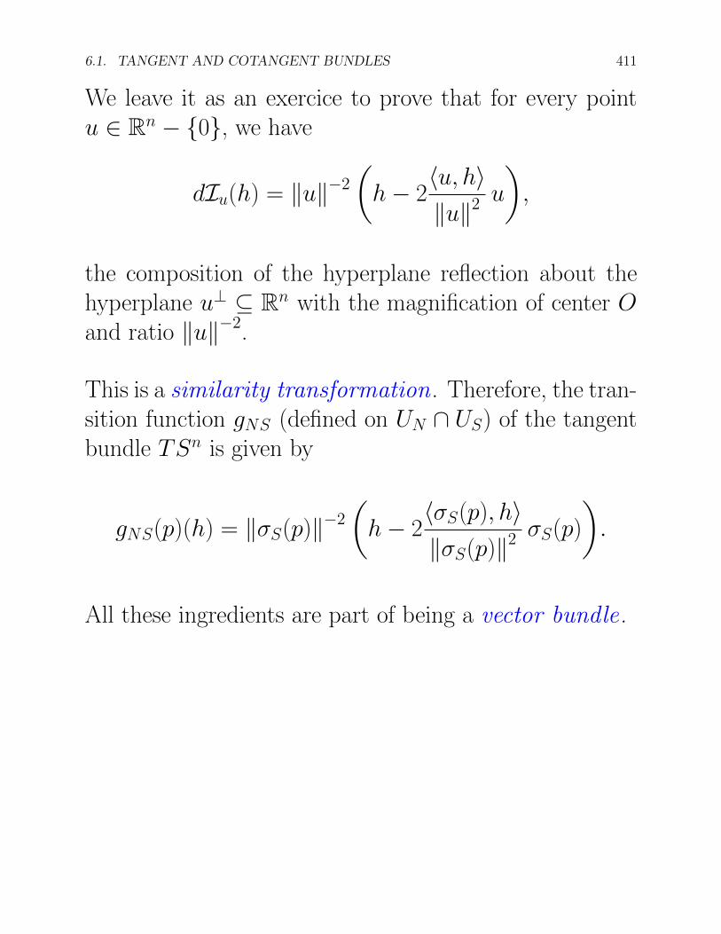
We leave it as an exercice to prove that for every pointu 2 Rn � {0}, we have
dIu(h) = kuk�2
✓h � 2
hu, hikuk2
u
◆,
the composition of the hyperplane reflection about thehyperplane u? ✓ Rn with the magnification of center Oand ratio kuk�2.
This is a similarity transformation. Therefore, the tran-sition function gNS (defined on UN \ US) of the tangentbundle TSn is given by
gNS(p)(h) = k�S(p)k�2
✓h � 2
h�S(p), hik�S(p)k2
�S(p)
◆.
All these ingredients are part of being a vector bundle .

412 CHAPTER 6. VECTOR FIELDS, INTEGRAL CURVES, FLOWS
For more on bundles, see Lang [23], Gallot, Hulin andLafontaine [17], Lafontaine [21] or Bott and Tu [5].
When M = Rn, observe thatT (M) = M ⇥ Rn = Rn ⇥ Rn, i.e., the bundle T (M) is(globally) trivial.
Given aCk-map, h : M ! N , between twoCk-manifolds,we can define the function, dh : T (M) ! T (N), (also de-noted Th, or h⇤, or Dh) by setting
dh(u) = dhp(u), i↵ u 2 Tp(M).
We leave the next proposition as an exercise to the reader(A proof can be found in Berger and Gostiaux [4]).
Proposition 6.1. Given a Ck-map, h : M ! N , be-tween two Ck-manifolds M and N (with k � 1), themap dh : T (M) ! T (N) is a Ck�1 map.
We are now ready to define vector fields.
6.2. VECTOR FIELDS, LIE DERIVATIVE 413
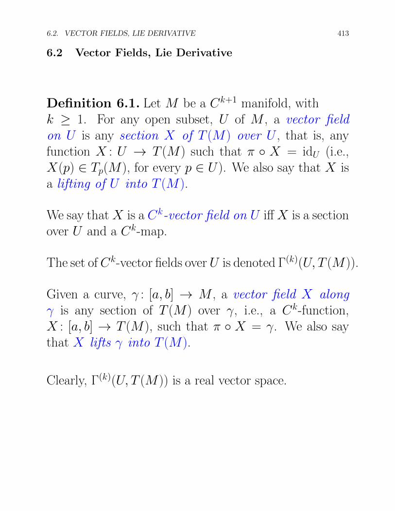
6.2 Vector Fields, Lie Derivative
Definition 6.1. Let M be a Ck+1 manifold, withk � 1. For any open subset, U of M , a vector fieldon U is any section X of T (M) over U , that is, anyfunction X : U ! T (M) such that ⇡ � X = idU (i.e.,X(p) 2 Tp(M), for every p 2 U). We also say that X isa lifting of U into T (M).
We say that X is a Ck-vector field on U i↵ X is a sectionover U and a Ck-map.
The set ofCk-vector fields overU is denoted �(k)(U, T (M)).
Given a curve, � : [a, b] ! M , a vector field X along� is any section of T (M) over �, i.e., a Ck-function,X : [a, b] ! T (M), such that ⇡ � X = �. We also saythat X lifts � into T (M).
Clearly, �(k)(U, T (M)) is a real vector space.
414 CHAPTER 6. VECTOR FIELDS, INTEGRAL CURVES, FLOWS
For short, the space �(k)(M, T (M)) is also denoted by�(k)(T (M)) (or X(k)(M), or even �(T (M)) or X(M)).
Remark: We can also define a Cj-vector field on U asa section, X , over U which is aCj-map, where 0 j k.Then, we have the vector space �(j)(U, T (M)), etc.
If M = Rn and U is an open subset of M , thenT (M) = Rn⇥Rn and a section of T (M) over U is simplya function, X , such that
X(p) = (p, u), with u 2 Rn,
for all p 2 U . In other words, X is defined by a function,f : U ! Rn (namely, f (p) = u).
This corresponds to the “old” definition of a vector fieldin the more basic case where the manifold, M , is just Rn.
6.2. VECTOR FIELDS, LIE DERIVATIVE 415
For any vector field X 2 �(k)(U, T (M)) and for any p 2U , we have X(p) = (p, v) for some v 2 Tp(M), andit is convenient to denote the vector v by Xp so thatX(p) = (p, Xp).
In fact, in most situations it is convenient to identify X(p)with Xp 2 Tp(M), and we will do so from now on.
This amounts to identifying the isomorphic vector spaces{p} ⇥ Tp(M) and Tp(M).
Let us illustrate the advantage of this convention with thenext definition.
Given any Ck-function, f 2 Ck(U), and a vector field,X 2 �(k)(U, T (M)), we define the vector field, fX , by
(fX)p = f (p)Xp, p 2 U.
416 CHAPTER 6. VECTOR FIELDS, INTEGRAL CURVES, FLOWS
Obviously, fX 2 �(k)(U, T (M)), which shows that�(k)(U, T (M)) is also a Ck(U)-module .
For any chart, (U,'), on M it is easy to check that themap
p 7!✓@
@xi
◆
p
, p 2 U,
is a Ck-vector field on U (with 1 i n). This vector
field is denoted⇣
@@xi
⌘or @
@xi.
6.2. VECTOR FIELDS, LIE DERIVATIVE 417
Definition 6.2. Let M be a Ck+1 manifold and let Xbe a Ck vector field on M . If U is any open subset of Mand f is any function in Ck(U), then the Lie derivativeof f with respect to X , denoted X(f ) or LXf , is thefunction on U given by
X(f )(p) = Xp(f ) = Xp(f), p 2 U.
Observe that
X(f )(p) = dfp(Xp),
where dfp is identified with the linear form in T ⇤p (M)
defined by
dfp(v) = v(f), v 2 TpM,
by identifying Tt0
R with R (see the discussion followingProposition 5.14).
The Lie derivative, LXf , is also denoted X [f ].

418 CHAPTER 6. VECTOR FIELDS, INTEGRAL CURVES, FLOWS
As a special case, when (U,') is a chart on M , the vectorfield, @
@xi, just defined above induces the function
p 7!✓@
@xi
◆
p
f, f 2 U,
denoted @@xi
(f ) or⇣
@@xi
⌘f .
It is easy to check that X(f ) 2 Ck�1(U).
As a consequence, every vector field X 2 �(k)(U, T (M))induces a linear map,
LX : Ck(U) �! Ck�1(U),
given by f 7! X(f ).
6.2. VECTOR FIELDS, LIE DERIVATIVE 419
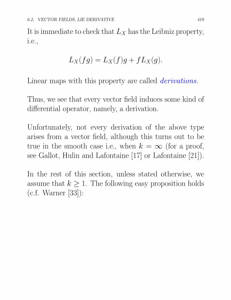
It is immediate to check that LX has the Leibniz property,i.e.,
LX(fg) = LX(f )g + fLX(g).
Linear maps with this property are called derivations .
Thus, we see that every vector field induces some kind ofdi↵erential operator, namely, a derivation.
Unfortunately, not every derivation of the above typearises from a vector field, although this turns out to betrue in the smooth case i.e., when k = 1 (for a proof,see Gallot, Hulin and Lafontaine [17] or Lafontaine [21]).
In the rest of this section, unless stated otherwise, weassume that k � 1. The following easy proposition holds(c.f. Warner [33]):

420 CHAPTER 6. VECTOR FIELDS, INTEGRAL CURVES, FLOWS
Proposition 6.2. Let X be a vector field on the Ck+1-manifold, M , of dimension n. Then, the following areequivalent:
(a) X is Ck.
(b) If (U,') is a chart on M and if f1
, . . . , fn are thefunctions on U uniquely defined by
X � U =nX
i=1
fi@
@xi,
then each fi is a Ck-map.
(c) Whenever U is open in M and f 2 Ck(U), thenX(f ) 2 Ck�1(U).
Given any two Ck-vector field, X, Y , on M , for any func-tion, f 2 Ck(M), we defined above the function X(f )and Y (f ).
Thus, we can form X(Y (f )) (resp. Y (X(f ))), which arein Ck�2(M).
6.2. VECTOR FIELDS, LIE DERIVATIVE 421
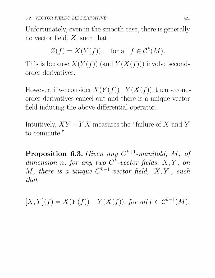
Unfortunately, even in the smooth case, there is generallyno vector field, Z, such that
Z(f ) = X(Y (f )), for all f 2 Ck(M).
This is because X(Y (f )) (and Y (X(f ))) involve second-order derivatives.
However, if we considerX(Y (f ))�Y (X(f )), then second-order derivatives cancel out and there is a unique vectorfield inducing the above di↵erential operator.
Intuitively, XY �Y X measures the “failure of X and Yto commute.”
Proposition 6.3. Given any Ck+1-manifold, M , ofdimension n, for any two Ck-vector fields, X, Y , onM , there is a unique Ck�1-vector field, [X, Y ], suchthat
[X, Y ](f ) = X(Y (f ))�Y (X(f )), for all f 2 Ck�1(M).

422 CHAPTER 6. VECTOR FIELDS, INTEGRAL CURVES, FLOWS
Definition 6.3. Given any Ck+1-manifold, M , of di-mension n, for any two Ck-vector fields, X, Y , on M , theLie bracket , [X, Y ], of X and Y , is the Ck�1 vector fielddefined so that
[X, Y ](f ) = X(Y (f ))�Y (X(f )), for all f 2 Ck�1(M).
An an example, in R3, if X and Y are the two vectorfields,
X =@
@x+ y
@
@zand Y =
@
@y,
then
[X, Y ] = � @
@z.
6.2. VECTOR FIELDS, LIE DERIVATIVE 423
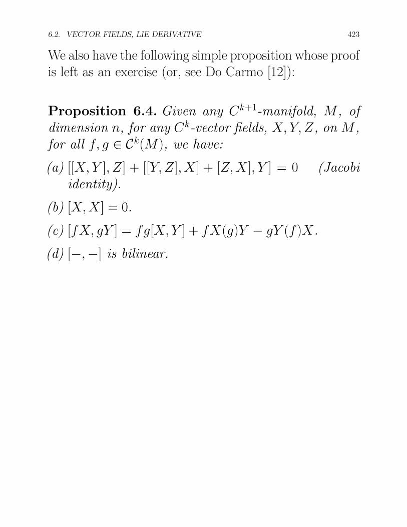
We also have the following simple proposition whose proofis left as an exercise (or, see Do Carmo [12]):
Proposition 6.4. Given any Ck+1-manifold, M , ofdimension n, for any Ck-vector fields, X, Y, Z, on M ,for all f, g 2 Ck(M), we have:
(a) [[X, Y ], Z] + [[Y, Z], X ] + [Z, X ], Y ] = 0 (Jacobiidentity).
(b) [X, X ] = 0.
(c) [fX, gY ] = fg[X, Y ] + fX(g)Y � gY (f )X.
(d) [�, �] is bilinear.

424 CHAPTER 6. VECTOR FIELDS, INTEGRAL CURVES, FLOWS
Consequently, for smooth manifolds (k = 1), the spaceof vector fields, �(1)(T (M)), is a vector space equippedwith a bilinear operation, [�, �], that satisfies the Jacobiidentity.
This makes �(1)(T (M)) a Lie algebra .
Let h : M ! N be a di↵eomorphism between two man-ifolds. Then, vector fields can be transported from N toM and conversely.

6.2. VECTOR FIELDS, LIE DERIVATIVE 425
Definition 6.4. Let h : M ! N be a di↵eomorphismbetween two Ck+1 manifolds. For every Ck vector field,Y , on N , the pull-back of Y along h is the vector field,h⇤Y , on M , given by
(h⇤Y )p = dh�1
h(p)
(Yh(p)
), p 2 M.
For every Ck vector field, X , on M , the push-forward ofX along h is the vector field, h⇤X , on N , given by
h⇤X = (h�1)⇤X,
that is, for every p 2 M ,
(h⇤X)h(p)
= dhp(Xp),
or equivalently,
(h⇤X)q = dhh�1
(q)(Xh�1
(q)), q 2 N.
426 CHAPTER 6. VECTOR FIELDS, INTEGRAL CURVES, FLOWS
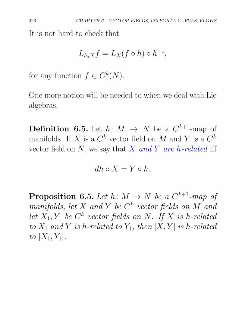
It is not hard to check that
Lh⇤Xf = LX(f � h) � h�1,
for any function f 2 Ck(N).
One more notion will be needed to when we deal with Liealgebras.
Definition 6.5. Let h : M ! N be a Ck+1-map ofmanifolds. If X is a Ck vector field on M and Y is a Ck
vector field on N , we say that X and Y are h-related i↵
dh � X = Y � h.
Proposition 6.5. Let h : M ! N be a Ck+1-map ofmanifolds, let X and Y be Ck vector fields on M andlet X
1
, Y1
be Ck vector fields on N . If X is h-relatedto X
1
and Y is h-related to Y1
, then [X, Y ] is h-relatedto [X
1
, Y1
].

6.3. INTEGRAL CURVES, FLOW, ONE-PARAMETER GROUPS 427
6.3 Integral Curves, Flow of a Vector Field,One-Parameter Groups of Di↵eomorphisms
We begin with integral curves and (local) flows of vectorfields on a manifold.
Definition 6.6. Let X be a Ck�1 vector field on a Ck-manifold, M , (k � 2) and let p
0
be a point on M . Anintegral curve (or trajectory) for X with initial con-dition p
0
is a Ck�1-curve, � : I ! M , so that
�(t) = X�(t), for all t 2 I and �(0) = p0
,
where I = ]a, b[ ✓ R is an open interval containing 0.
What definition 6.6 says is that an integral curve, �, withinitial condition p
0
is a curve on the manifold M passingthrough p
0
and such that, for every point p = �(t) onthis curve, the tangent vector to this curve at p, i.e., �(t),coincides with the value, Xp, of the vector field X at p.

428 CHAPTER 6. VECTOR FIELDS, INTEGRAL CURVES, FLOWS
Given a vector field, X , as above, and a point p0
2 M ,is there an integral curve through p
0
? Is such a curveunique? If so, how large is the open interval I?
We provide some answers to the above questions below.
Definition 6.7. Let X be a Ck�1 vector field on a Ck-manifold, M , (k � 2) and let p
0
be a point on M . Alocal flow for X at p
0
is a map,
' : J ⇥ U ! M,
where J ✓ R is an open interval containing 0 and U is anopen subset of M containing p
0
, so that for every p 2 U ,the curve t 7! '(t, p) is an integral curve of X with initialcondition p.
Thus, a local flow for X is a family of integral curvesfor all points in some small open set around p
0
such thatthese curves all have the same domain, J , independentlyof the initial condition, p 2 U .

6.3. INTEGRAL CURVES, FLOW, ONE-PARAMETER GROUPS 429
The following theorem is the main existence theorem oflocal flows.
This is a promoted version of a similar theorem in theclassical theory of ODE’s in the case where M is an opensubset of Rn.
Theorem 6.6. (Existence of a local flow) Let X be aCk�1 vector field on a Ck-manifold, M , (k � 2) andlet p
0
be a point on M . There is an open interval J ✓R containing 0 and an open subset U ✓ M containingp
0
, so that there is a unique local flow ' : J ⇥U ! Mfor X at p
0
.
What this means is that if '1
: J⇥U ! M and '2
: J⇥U ! M are both local flows with domain J ⇥ U , then'
1
= '2
. Furthermore, ' is Ck�1.

430 CHAPTER 6. VECTOR FIELDS, INTEGRAL CURVES, FLOWS
Theorem 6.6 holds under more general hypotheses, namely,when the vector field satisfies some Lipschitz condition,see Lang [23] or Berger and Gostiaux [4].
Now, we know that for any initial condition, p0
, there issome integral curve through p
0
.
However, there could be two (or more) integral curves�
1
: I1
! M and �2
: I2
! M with initial condition p0
.
This leads to the natural question: How do �1
and �2
di↵er on I1
\ I2
? The next proposition shows they don’t!
Proposition 6.7. Let X be a Ck�1 vector field on aCk-manifold, M , (k � 2) and let p
0
be a point on M .If �
1
: I1
! M and �2
: I2
! M are any two integralcurves both with initial condition p
0
, then �1
= �2
onI1
\ I2
.

6.3. INTEGRAL CURVES, FLOW, ONE-PARAMETER GROUPS 431
Proposition 6.7 implies the important fact that there is aunique maximal integral curve with initial condition p.
Indeed, if {�j : Ij ! M}j2K is the family of all integralcurves with initial condition p (for some big index set,K), if we let I(p) =
Sj2K Ij, we can define a curve,
�p : I(p) ! M , so that
�p(t) = �j(t), if t 2 Ij.
Since �j and �l agree on Ij \ Il for all j, l 2 K, the curve�p is indeed well defined and it is clearly an integral curvewith initial condition p with the largest possible domain(the open interval, I(p)).
The curve �p is called the maximal integral curve withinitial condition p and it is also denoted by �(p, t).
Note that Proposition 6.7 implies that any two distinct in-tegral curves are disjoint, i.e., do not intersect each other.

432 CHAPTER 6. VECTOR FIELDS, INTEGRAL CURVES, FLOWS
Consider the vector field in R2 given by
X = �y@
@x+ x
@
@y
and shown in Figure 6.1.
Figure 6.1: A vector field in R2
If we write �(t) = (x(t), y(t)), the di↵erential equation,�(t) = X(�(t)), is expressed by
x0(t) = �y(t)
y0(t) = x(t),
or, in matrix form,✓
x0
y0
◆=
✓0 �11 0
◆✓x
y
◆.
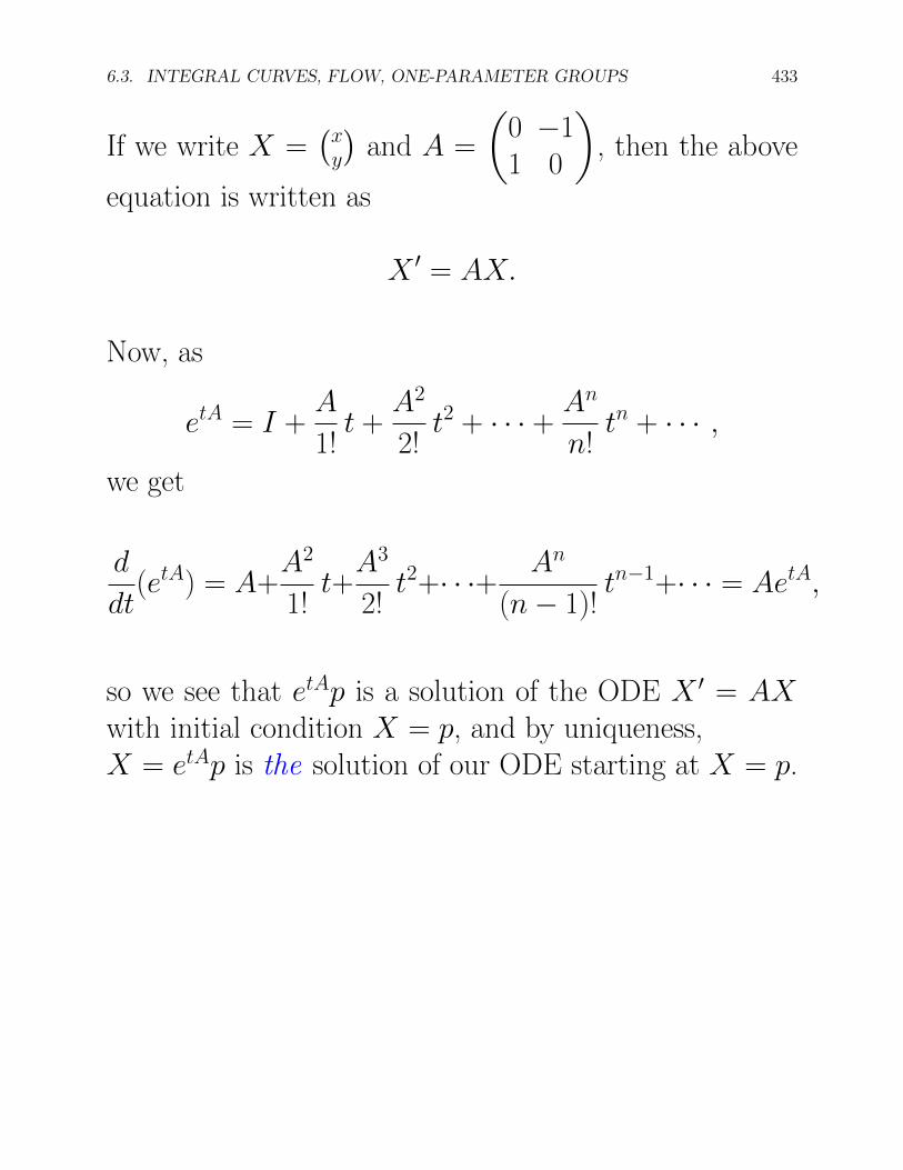
6.3. INTEGRAL CURVES, FLOW, ONE-PARAMETER GROUPS 433
If we write X =�x
y
�and A =
✓0 �11 0
◆, then the above
equation is written as
X 0 = AX.
Now, as
etA = I +A
1!t +
A2
2!t2 + · · · + An
n!tn + · · · ,
we get
d
dt(etA) = A+
A2
1!t+
A3
2!t2+· · ·+ An
(n � 1)!tn�1+· · · = AetA,
so we see that etAp is a solution of the ODE X 0 = AXwith initial condition X = p, and by uniqueness,X = etAp is the solution of our ODE starting at X = p.
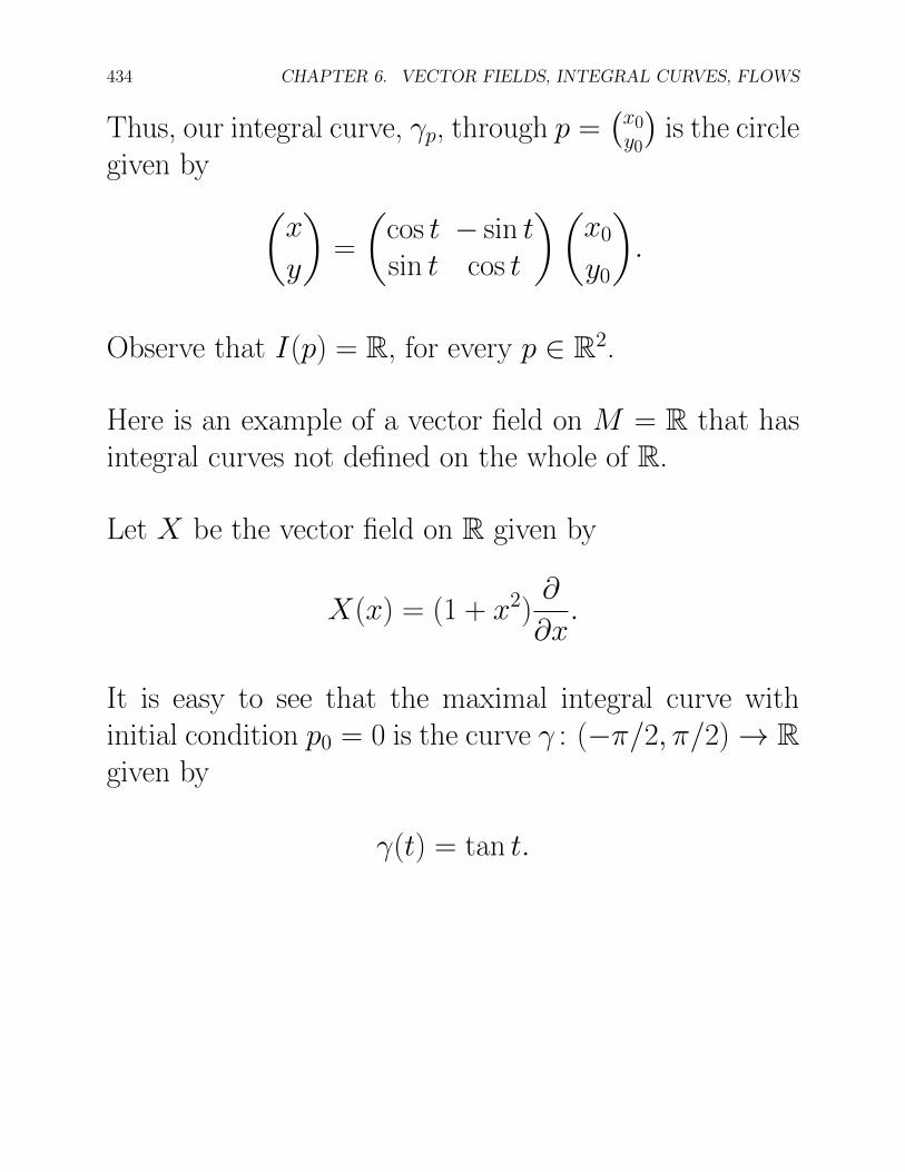
434 CHAPTER 6. VECTOR FIELDS, INTEGRAL CURVES, FLOWS
Thus, our integral curve, �p, through p =�x
0
y0
�is the circle
given by✓
x
y
◆=
✓cos t � sin tsin t cos t
◆✓x
0
y0
◆.
Observe that I(p) = R, for every p 2 R2.
Here is an example of a vector field on M = R that hasintegral curves not defined on the whole of R.
Let X be the vector field on R given by
X(x) = (1 + x2)@
@x.
It is easy to see that the maximal integral curve withinitial condition p
0
= 0 is the curve � : (�⇡/2, ⇡/2) ! Rgiven by
�(t) = tan t.

6.3. INTEGRAL CURVES, FLOW, ONE-PARAMETER GROUPS 435
The following interesting question now arises: Given anyp
0
2 M , if �p0
: I(p0
) ! M is the maximal integralcurve with initial condition p
0
and, for any t1
2 I(p0
), ifp
1
= �p0
(t1
) 2 M , then there is a maximal integral curve,�p
1
: I(p1
) ! M , with initial condition p1
;
What is the relationship between �p0
and �p1
, if any?
The answer is given by
Proposition 6.8. Let X be a Ck�1 vector field ona Ck-manifold, M , (k � 2) and let p
0
be a pointon M . If �p
0
: I(p0
) ! M is the maximal integralcurve with initial condition p
0
, for any t1
2 I(p0
), ifp
1
= �p0
(t1
) 2 M and �p1
: I(p1
) ! M is the maximalintegral curve with initial condition p
1
, then
I(p1
) = I(p0
)�t1
and �p1
(t) = ��p0
(t1
)
(t) = �p0
(t+t1
),
for all t 2 I(p0
) � t1

436 CHAPTER 6. VECTOR FIELDS, INTEGRAL CURVES, FLOWS
Proposition 6.8 says that the traces �p0
(I(p0
)) and�p
1
(I(p1
)) inM of the maximal integral curves �p0
and �p1
are identical; they only di↵er by a simple reparametriza-tion (u = t + t
1
).
It is useful to restate Proposition 6.8 by changing pointof view.
So far, we have been focusing on integral curves, i.e., givenany p
0
2 M , we let t vary in I(p0
) and get an integralcurve, �p
0
, with domain I(p0
).
6.3. INTEGRAL CURVES, FLOW, ONE-PARAMETER GROUPS 437
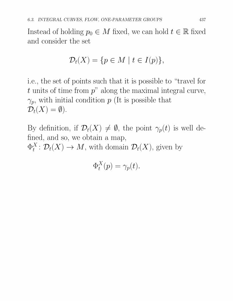
Instead of holding p0
2 M fixed, we can hold t 2 R fixedand consider the set
Dt(X) = {p 2 M | t 2 I(p)},
i.e., the set of points such that it is possible to “travel fort units of time from p” along the maximal integral curve,�p, with initial condition p (It is possible thatDt(X) = ;).
By definition, if Dt(X) 6= ;, the point �p(t) is well de-fined, and so, we obtain a map,�X
t : Dt(X) ! M , with domain Dt(X), given by
�Xt (p) = �p(t).

438 CHAPTER 6. VECTOR FIELDS, INTEGRAL CURVES, FLOWS
Definition 6.8. Let X be a Ck�1 vector field on a Ck-manifold, M , (k � 2). For any t 2 R, let
Dt(X) = {p 2 M | t 2 I(p)}
andD(X) = {(t, p) 2 R ⇥ M | t 2 I(p)}
and let �X : D(X) ! M be the map given by
�X(t, p) = �p(t).
The map �X is called the (global) flow of X and D(X)is called its domain of definition .
For any t 2 R such that Dt(X) 6= ;, the map, p 2Dt(X) 7! �X(t, p) = �p(t), is denoted by �X
t (i.e.,
�Xt (p) = �X(t, p) = �p(t)).
6.3. INTEGRAL CURVES, FLOW, ONE-PARAMETER GROUPS 439
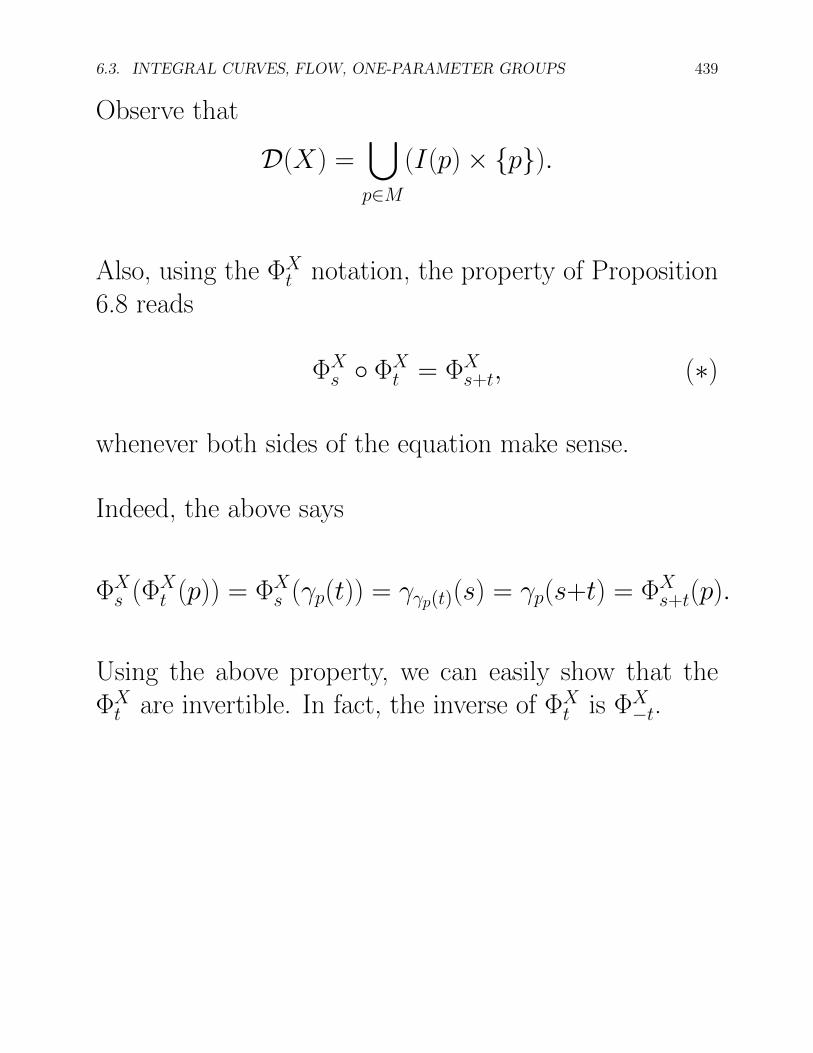
Observe that
D(X) =[
p2M
(I(p) ⇥ {p}).
Also, using the �Xt notation, the property of Proposition
6.8 reads
�Xs � �X
t = �Xs+t, (⇤)
whenever both sides of the equation make sense.
Indeed, the above says
�Xs (�
Xt (p)) = �X
s (�p(t)) = ��p(t)(s) = �p(s+t) = �Xs+t(p).
Using the above property, we can easily show that the�X
t are invertible. In fact, the inverse of �Xt is �X
�t.

440 CHAPTER 6. VECTOR FIELDS, INTEGRAL CURVES, FLOWS
Theorem 6.9. Let X be a Ck�1 vector field on a Ck-manifold, M , (k � 2). The following properties hold:
(a) For every t 2 R, if Dt(X) 6= ;, then Dt(X) is open(this is trivially true if Dt(X) = ;).
(b) The domain, D(X), of the flow, �X, is open andthe flow is a Ck�1 map, �X : D(X) ! M .
(c) Each �Xt : Dt(X) ! D�t(X) is a Ck�1-di↵eomor-
phism with inverse �X�t.
(d) For all s, t 2 R, the domain of definition of�X
s � �Xt is contained but generally not equal to
Ds+t(X). However, dom(�Xs � �X
t ) = Ds+t(X) if sand t have the same sign. Moreover, ondom(�X
s � �Xt ), we have
�Xs � �X
t = �Xs+t.
We may omit the superscript, X , and write � instead of�X if no confusion arises.
6.3. INTEGRAL CURVES, FLOW, ONE-PARAMETER GROUPS 441
The reason for using the terminology flow in referring tothe map �X can be clarified as follows:
For any t such that Dt(X) 6= ;, every integral curve, �p,with initial condition p 2 Dt(X), is defined on some openinterval containing [0, t], and we can picture these curvesas “flow lines” along which the points p flow (travel) fora time interval t.
Then, �X(t, p) is the point reached by “flowing” for theamount of time t on the integral curve �p (through p)starting from p.
Intuitively, we can imagine the flow of a fluid throughM , and the vector field X is the field of velocities of theflowing particles.
442 CHAPTER 6. VECTOR FIELDS, INTEGRAL CURVES, FLOWS
Given a vector field, X , as above, it may happen thatDt(X) = M , for all t 2 R.
In this case, namely, when D(X) = R ⇥ M , we say thatthe vector field X is complete .
Then, the �Xt are di↵eomorphisms of M and they form
a group.
The family {�Xt }t2R a called a 1-parameter group of X .
In this case, �X induces a group homomorphism,(R,+) �! Di↵(M), from the additive group R to thegroup of Ck�1-di↵eomorphisms of M .
By abuse of language, even when it is not the case thatDt(X) = M for all t, the family {�X
t }t2R is called a local1-parameter group of X , even though it is not a group,because the composition �X
s � �Xt may not be defined.

6.3. INTEGRAL CURVES, FLOW, ONE-PARAMETER GROUPS 443
If we go back to the vector field in R2 given by
X = �y@
@x+ x
@
@y,
since the integral curve, �p(t), through p =�x
0
x0
�is given
by✓
x
y
◆=
✓cos t � sin tsin t cos t
◆✓x
0
y0
◆,
the global flow associated with X is given by
�X(t, p) =
✓cos t � sin tsin t cos t
◆p,
and each di↵eomorphism, �Xt , is the rotation,
�Xt =
✓cos t � sin tsin t cos t
◆.

444 CHAPTER 6. VECTOR FIELDS, INTEGRAL CURVES, FLOWS
The 1-parameter group, {�Xt }t2R, generated by X is the
group of rotations in the plane, SO(2).
More generally, if B is an n⇥n invertible matrix that hasa real logarithm A (that is, if eA = B), then the matrixA defines a vector field, X , in Rn, with
X =nX
i,j=1
(aijxj)@
@xi,
whose integral curves are of the form,
�p(t) = etAp,
and we have�p(1) = Bp.
The one-parameter group, {�Xt }t2R, generated by X is
given by {etA}t2R.
6.3. INTEGRAL CURVES, FLOW, ONE-PARAMETER GROUPS 445
When M is compact, it turns out that every vector fieldis complete, a nice and useful fact.
Proposition 6.10. Let X be a Ck�1 vector field on aCk-manifold, M , (k � 2). If M is compact, then Xis complete, i.e., D(X) = R⇥ M . Moreover, the mapt 7! �X
t is a homomorphism from the additive groupR to the group, Di↵(M), of (Ck�1) di↵eomorphismsof M .
Remark: The proof of Proposition 6.10 also applies whenX is a vector field with compact support (this means thatthe closure of the set {p 2 M | X(p) 6= 0} is compact).
If h : M ! N is a di↵eomorphism and X is a vector fieldon M , it can be shown that the local 1-parameter groupassociated with the vector field, h⇤X , is
{h � �Xt � h�1}t2R.

446 CHAPTER 6. VECTOR FIELDS, INTEGRAL CURVES, FLOWS
A point p 2 M where a vector field vanishes, i.e.,X(p) = 0, is called a critical point of X .
Critical points play a major role in the study of vec-tor fields, in di↵erential topology (e.g., the celebratedPoincare–Hopf index theorem) and especially in Morsetheory, but we won’t go into this here.
Another famous theorem about vector fields says thatevery smooth vector field on a sphere of even dimension(S2n) must vanish in at least one point (the so-called“hairy-ball theorem.”
On S2, it says that you can’t comb your hair withouthaving a singularity somewhere. Try it, it’s true!).
6.3. INTEGRAL CURVES, FLOW, ONE-PARAMETER GROUPS 447
Let us just observe that if an integral curve, �, passesthrough a critical point, p, then � is reduced to the pointp, i.e., �(t) = p, for all t.
Then, we see that if a maximal integral curve is definedon the whole of R, either it is injective (it has no self-intersection), or it is simply periodic (i.e., there is someT > 0 so that �(t + T ) = �(t), for all t 2 R and � isinjective on [0, T [ ), or it is reduced to a single point.
We conclude this section with the definition of the Liederivative of a vector field with respect to another vectorfield.
448 CHAPTER 6. VECTOR FIELDS, INTEGRAL CURVES, FLOWS
Say we have two vector fields X and Y on M . For anyp 2 M , we can flow along the integral curve of X withinitial condition p to �t(p) (for t small enough) and thenevaluate Y there, getting Y (�t(p)).
Now, this vector belongs to the tangent space T�t(p)
(M),but Y (p) 2 Tp(M).
So to “compare” Y (�t(p)) and Y (p), we bring back Y (�t(p))to Tp(M) by applying the tangent map, d��t, at �t(p),to Y (�t(p)). (Note that to alleviate the notation, we usethe slight abuse of notation d��t instead of d(��t)
�t(p)
.)

6.3. INTEGRAL CURVES, FLOW, ONE-PARAMETER GROUPS 449
Then, we can form the di↵erence d��t(Y (�t(p)))�Y (p),divide by t and consider the limit as t goes to 0.
Definition 6.9. Let M be a Ck+1 manifold. Given anytwo Ck vector fields, X and Y on M , for every p 2 M ,the Lie derivative of Y with respect to X at p, denoted(LX Y )p, is given by
(LX Y )p = limt�!0
d��t(Y (�t(p))) � Y (p)
t
=d
dt(d��t(Y (�t(p))))
����t=0
.
It can be shown that (LX Y )p is our old friend, the Liebracket, i.e.,
(LX Y )p = [X, Y ]p.
(For a proof, see Warner [33] or O’Neill [30]).

450 CHAPTER 6. VECTOR FIELDS, INTEGRAL CURVES, FLOWS
In terms of Definition 6.4, observe that
(LX Y )p = limt�!0
�(��t)⇤Y
�(p) � Y (p)
t
= limt�!0
��⇤
t Y�(p) � Y (p)
t
=d
dt
��⇤
t Y�(p)
����t=0
,
since (��t)�1 = �t.