Chapter 6: The Mathematics of Touring 6.1 What Is a Traveling Salesman Problem?

Chapter 6:The Mathematics of Touring

6.1 What Is a Traveling Salesman Problem?

Excursions in Modern Mathematics, 7e: 1.1 - 2Copyright © 2010 Pearson Education, Inc.Copyright © 2014 Pearson Education. All rights reserved. 6.1-2

The “traveling salesman” is a convenient metaphor for many different real-life applications. The next few examples illustrate a few of the many possible settingsfor a “traveling salesman” problem, starting, of course, with the traveling salesman’s “traveling salesman” problem.

Traveling Salesman Problems


Meet Willy, the traveling salesman. Willy has customers in five cities, which for the sake of brevity we will call A, B, C, D, and E. Willy needs to schedule a sales trip that will start and end at A (that’s Willy’s hometown) and goes to each of the other four cities once. We will call the trip “Willy’s sales tour.” Other than starting and ending at A, there are no restrictions as to the sequence in which Willy’s sales tour visits the other four cities.

Example 6.4 A Tour of Five Cities


The graph shows the cost of a one-way airline ticket between each pair of cities. Like most people, Willy hates to waste money.

Example 6.4 A Tour of Five Cities

Thus, among the many possibilities for his sales tour, Willy wants to find the optimal (cheapest) one. How? We will return to this question soon.


It is the year 2020. An expedition to explore the outer planetary moons in our solar system is about to be launched from planet Earth. The expedition is scheduled to visit Callisto, Ganymede, Io, Mimas, and Titan (the first three are moons of Jupiter; the last two, of Saturn), collect rock samples at each, and then return to Earth with the loot. The next slide shows the mission time (in years) between any two moons. An important goal of the mission planners is to complete the mission in the least amount of time.

Example 6.5 Touring the Outer Moons


What is the optimal (shortest) tourof the outer moons?

Example 6.5 Touring the Outer Moons


The figure shows seven locations on Mars where NASA scientists believe there is a good chance of finding evidence of life.

Example 6.6 Roving the Red Planet


Imagine that you are in charge of planning a sample-return mission. First, you must land an unmanned rover in the Ares Vallis (A). Then you must direct the rover to travel to each site and collect and analyze soil samples. Finally, you must instruct the rover to return to the Ares Vallis landing site, where a return rocket will bring the best samples back to Earth. A Mars tour like this will take several years and cost several billion dollars, so good planning is critical.



Here are the estimated distances (in miles) that a roverwould have to travel to get from one Martian site to another. What is the optimal (shortest) tour for the Mars rover?



In each case the problem is to find a tour of the sites (i.e., a trip that starts and ends at a designated site and visits each of the other sites once) and has the property of being optimal (i.e., has the least total cost). Any problem that shares these common elements (a traveler, a set of sites, a cost function for travel between pairs of sites, a need to tour all the sites, and a desire to minimize the total cost of the tour) is known as a traveling salesman problem, or TSP.

Traveling Salesman Examples


A school bus (the traveler) picks up children in the morning and drops them off at the end of the day atdesignated stops (the sites). On a typical school bus route there may be 20 to 30 such stops. With school buses, total time on the bus is always the most important variable (students have to get to school on time), and there is a known time of travel (the cost) between any two bus stops. Since children must be picked up at every bus stop, a tour of all the sites (starting and ending at the school) is required. Since thebus repeats its route every day during the school year,finding an optimal tour is crucial.

Routing School Buses


Package delivery companies such as UPS and FedEx deal with TSPs on a daily basis. Each truck is a traveler that must deliver packages to a specific list of delivery destinations (the sites). The travel time between any two delivery sites (the cost) is known or can be estimated. Each day the truck must deliver to all the sites on its list (that’s why sometimes you see a UPS truckdelivering at 8 P.M.), so a tour is an implied part of the requirements. Since one can assume that the driver would rather be home than out delivering packages, an optimal tour is a highly desirable goal.

Delivering Packages


In the process of fabricating integrated-circuit boards, tens of thousands of tiny holes (the sites) must be drilled in each board. This is done by using a stationary laser beam and moving the board (the traveler). To do this efficiently, the order in which the holes are drilled shouldbe such that the entire drilling sequence (the tour) is completed in the least amount of time (optimal cost). This makes for a very high tech TSP.

Fabricating Circuit Boards


On a typical Saturday morning, an average Joe or Jane (the traveler) sets out to run a bunch of errands around town, visiting various sites (grocery store, hair salon, bakery, post office). When gas was cheap, time used to be the key cost variable, but with the cost of gas these days, people are more likely to be looking forthe tour that minimizes the total distance traveled.

Fabricating Circuit Boards


Every TSP can be modeled by a weighted graph, that is, a graph such that there is a number associated with each edge (called the weight of the edge). The beauty of this approach is that the model always has the samestructure: The vertices of the graph are the sites of the TSP, and there is an edge between X and Y if there is a direct link for the traveler to travel from site X to site Y. Moreover, the weight of the edge XY is the cost of travel between X and Y.

Modeling a TSP


In this setting a tour is a Hamilton circuit of the graph, and an optimal tour is the Hamilton circuit of least total weight. In all the applications and examples we will be considering in this chapter, we will make the assumptionthat there is an edge connecting every pair of sites, which implies that the underlying graph model is always a complete weighted graph. The following is a summary of the preceding observations.

Modeling a TSP


■ Sites g vertices of the graph.

■ Costs g weights of the edges.

■ Tour g Hamilton circuit.

■ Optimal tour g Hamilton circuit of least total cost

GRAPH MODEL OF A TRAVELING SALESMAN PROBLEM



6.2 Hamilton Paths and Circuits


In Chapter 5 we discussed Euler paths and Euler circuits. There, the name of the game was to find paths or circuits that include every edge of the graph once (and only once). We are now going to discuss a seemingly related game: finding paths and circuits that include every vertex of the graph once and only once. Paths and circuits having this property are called Hamilton paths and Hamilton circuits.

Hamilton Paths and Hamilton Circuits


■ A Hamilton path in a graph is a path that includes each vertex of the graph once and only once.

■ A Hamilton circuit is a circuit that includes each vertex of the graph once and only once. (At the end, of course, the circuit must return to the starting vertex.)

HAMILTON PATHS & CIRCUITS


On the surface, there is a one-word difference between Euler paths/circuits and Hamilton paths/circuits: The former covers all edges; the latter covers all vertices.

But oh my, what a difference that one word makes!

Euler vs. Hamilton Paths & Circuits


The figure shows a graph that (1) has Euler circuits (the vertices areall even) and (2) has Hamilton circuits.

Example 6.1 Hamilton versus Euler

One such Hamilton circuit is A,F, B, C, G, D, E, A – there are plenty more.


Note that if a graph has a Hamilton circuit, then it automatically has a Hamilton path–the Hamilton circuitcan always be truncated into a Hamilton path by dropping the last vertex of the circuit. (For example, the Hamilton circuit A, F, B, C, G, D, E, A can be truncated into the Hamilton path A, F, B, C, G, D, E.) Contrast this with the mutually exclusive relationship between Euler circuits and paths: If a graph has an Euler circuit it cannot have an Euler path and vice versa.



This figure shows a graph that (1) has no Euler circuitsbut does have Euler paths (for example C, D, E, B, A, D) and (2) has no Hamilton circuits (sooner or later you have to go to C, and then you are stuck) but does


have Hamilton paths (for example, A, B, E, D, C). This illustrates that a graph can have a Hamilton path but no Hamilton circuit!


This figure shows a graph that (1) has neither Euler circuits nor paths (it has four odd vertices) and (2) has Hamilton circuits (for example A, B, C, D, E, A – there areplenty more) and consequently


has Hamilton paths (for example, A, B, C, D, E).


This figure shows a graph that (1) has Euler circuits (the vertices are all even) and (2) has no Hamilton circuits (no matter what, you are going to have to go through E more than once!)


but has Hamilton paths (for example, A, B, E, D, C).


This figure shows a graph that

(1) has no Euler circuits but has Euler paths (F and G are the two odd vertices) and

(2) has neither Hamilton circuits nor Hamilton paths.



This figure shows a graph that

(1) has neither Euler circuits nor Euler paths (too many odd vertices) and

(2) has neither Hamilton circuits nor Hamilton paths.



Summary


The lesson of Example 6.1 is that the existence of an Euler path or circuit in a graph tells us nothing about the existence of a Hamilton path or circuit in that graph. This is important because it implies that Euler’s circuit and path theorems from Chapter 5 are useless when it comes to identifying Hamilton circuits and paths. But surely, there must be analogous “Hamilton circuit and path theorems” that we could use to determine if a graph has a Hamilton circuit, a Hamilton path, or neither.

Euler versus Hamilton


Surprisingly, no such theorems exist. Determining whena given graph does or does not have a Hamilton circuit or path can be very easy, but it also can be very hard–it all depends on the graph.

Euler versus Hamilton



6.3 The Brute to Force Algorithm


In this section we will look at the two strategies we informally developed in connection with Willy’s sales trips and recast them in the language of algorithms. The“exhaustive search” strategy can be formalized into an algorithm generally known as the brute-force algorithm; the “go cheap” strategy can be formalized into an algorithm known as the nearest-neighbor algorithm.

Algorithms for Solving TSP’s


■ Step 1. Make a list of all the possible Hamilton circuits of the graph. Each of these circuits represents a tour of the vertices of the graph.

■ Step 2. For each tour calculate its weight (i.e., add the weights of all the edges in the circuit).

■ Step 3. Choose an optimal tour (there is always more than one optimal tour to choose from!).

ALGORITHM 1: THE BRUTE FORCE ALGORITHM


The positive aspect of the brute-force algorithm is that it is an optimal algorithm. (An optimal algorithm isan algorithm that, when correctly implemented, is guaranteed to produce an optimal solution.) In the case of the brute-force algorithm, we know we are getting an optimal solution because we are choosingfrom among all possible tours.

Pros and Cons


The negative aspect of the brute-force algorithm is the amount of effort that goes into implementing the algorithm, which is (roughly) proportional to the number of Hamilton circuits in the graph. As we first saw in Table 6-4, as the number of vertices grows just a little, the number of Hamilton circuits in a complete graph grows at an incredibly fast rate.

Pros and Cons


What does this mean in practical terms? Let’s start with human computation. To solve a TSP for a graph with 10 vertices (as real-life problems go, that’s puny), the brute-force algorithm requires checking 362,880 Hamilton circuits. To do this by hand, even for a fast and clever human, it would take over 1000 hours. Thus, N =10 at we are already beyond the limit of what can be considered reasonable human effort.

Practical Terms of the Pros and Cons


Even with the world’s best technology on our side, we very quickly reach the point beyond which using the brute-force algorithm is completely unrealistic.

Using a Computer


The brute-force algorithm is a classic example of what is formally known as an inefficient algorithm–an algorithm for which the number of steps needed to carry it out grows disproportionately with the size of the problem. The trouble with inefficient algorithms is that they are of limited practical use–they can realistically be carried out only when the problem is small.

Using a Computer


We hop from vertex to vertex using a simple criterion: Choose the next available “nearest” vertex and go for it. Let’s call the process of checking among the available vertices and finding the nearest one a single computation. Then, for a TSP with N = 5 we need to perform 5 computations. What happens when we double, the number of vertices to N = 10? We now have to perform 10 computations. For N = 30, we perform 30 computations.

Pros and Cons - Nearest Neighbor


We can summarize the above observations by saying that the nearest-neighbor algorithm is an efficient algorithm. Roughly speaking, an efficient algorithm is an algorithm for which the amount of computational effort required to implement the algorithm grows in some reasonable proportion with the size of the input to the problem.



The main problem with the nearest-neighbor algorithm is that it is not an optimal algorithm. In Example 6.7, the nearest-neighbor tour had a cost of $773, whereas the optimal tour had a cost of $676. In absolute terms the nearest-neighbor tour is off by $97 (this is called the absolute error). A better way to describe how far “off” this tour is from the optimal tour is to use the concept of relative error. In this example the absolute error is $97 out of $676, giving a relative error of $97/$676 = 0.1434911 ≈ 14.35%.



In general, for any tour that might be proposed as a“solution” to a TSP, we can find its relative error as follows:

RELATIVE ERROR OF A TOUR (e)

cost of tour cost of optimal tour cost of optimal tour


It is customary to express the relative error as a percentage (usually rounded to two decimal places). By using the notion of relative error, we can characterize the optimal tours as those with relative error of 0%. All other tours give “approximate solutions,” the relative merits of which we can judge by their respective relative errors: tours with “small” relative errors are good, and tours with “large” relative errors are not good.

Relative Error - Good or Not Good


Chapter 6:The Mathematics of Touring6.4 The Nearest to Neighbor and Repetitive Nearest to Neighbor Algorithms


■ Start: Start at the designated starting vertex. If there is no designated starting vertex pick any vertex.

■ First step: From the starting vertex go to its nearest neighbor (i.e., the vertex for which the corresponding edge has the smallest weight).

ALGORITHM 2: THE NEAREST NEIGHBOR ALGORITHM


■ Middle steps: From each vertex go to its nearest neighbor, choosing only among the vertices that haven’t been yet visited. (If there is more than one nearest neighbor choose among them at random.) Keep doing this until all the vertices have been visited.

■ Last step: From the last vertex return to the starting vertex.

ALGORITM 2: THE NEAREST NEIGHBOR ALGORITHM


As one might guess, the repetitive nearest-neighbor algorithm is a variation of the nearest-neighbor algorithm in which we repeat several times the entirenearest- neighbor circuit-building process. Why would we want to do this? The reason is that the nearest-neighbor tour depends on the choice of the starting vertex. If we change the starting vertex, the nearest-neighbor tour is likely to be different, and, if we are lucky, better.

Repetitive Nearest-Neighbor Algorithm


Since finding a nearest-neighbor tour is an efficient process, it is not unreasonable to repeat the process several times, each time starting at a different vertex of the graph. In this way, we can obtain several different “nearest-neighbor solutions,” from which we can then pick the best.



But what do we do with a tour that starts somewhere other than the vertex we really want to start at? That’s not a problem. Remember that once we have a circuit,we can start the circuit anywhere we want. In fact, in an abstract sense, a circuit has no starting or ending point.



In Example 6.7, we computed the nearest-neighbor tour with A as the starting vertex, and we got A, C, E, D, B, A with a total cost of $773.

Example 6.10A Tour of Five Cities: Part 3


But if we use B as the starting vertex, the nearest-neighbor tour takes us from B to C, then to A, E, D, and back to B, with a total cost of $722. Well, that is certainly an improvement!


As for Willy–who must start and end his trip at A–this very same tour would take the form A, E, D, B, C, A.


The process is once again repeated using C, D, and E as the starting vertices. When the starting point is C, we get the nearest-neighbor tour C, A, E, D, B, C (total cost is $722); when the starting point is D, we get the nearest-neighbor tour D, B, C, A, E, D (total cost is $722); and when the starting point is E, we get the nearest-neighbor tour E, C, A, D, B, E (total cost is $741).



Among all the nearest-neighbor tours we pick the cheapest one – A, E, D, B, C, A – with a cost of $722.



■ Let X be any vertex. Find the nearest-neighbor tour with X as the starting vertex, and calculate the cost of this tour.

■ Repeat the process with each of the other vertices of the graph as the starting vertex.

■ Of the nearest-neighbor tours thus obtained, choose one with least cost. If necessary, rewrite the tour so that it starts at the designated starting vertex. We will call this tour the repetitive nearest-neighbor tour.

ALGORITHM 3: THE REPETITIVE NEAREST NEIGHBOR ALGORITHM



6.5 The Cheapest to Link Algorithm


The idea behind the cheapest-link algorithm is to piece together a tour by picking the separate “links” (i.e., legs) of the tour on the basis of cost. It doesn’t matter ifin the intermediate stages the “links” are all over the place – if we are careful at the end, they will all come together and form a tour. This is how it works: Look at the entire graph and choose the cheapest edge of the graph, wherever that edge may be. Once this is done, choose the next cheapest edge of the graph, wherever that edge may be.

Cheapest-Link Algorithm


(Don’t worry if that edge is not adjacent to the first edge.) Continue this way, each time choosing the cheapest edge available but following two rules:

(1) Do not allow a circuit to form except at the very end, and

(2) do not allow three edges to come together at a vertex.

A violation of either of these two rules will prevent forming a Hamilton circuit. Conversely, following these two rules guarantees that the end result will be a Hamilton circuit.

Cheapest-Link Algorithm


Since finding a nearest-neighbor tour is an efficient process, it is not unreasonable to repeat the process several times, each time starting at a different vertex of the graph. In this way, we can obtain several different “nearest-neighbor solutions,” from which we can then pick the best.



But what do we do with a tour that starts somewhere other than the vertex we really want to start at? That’s not a problem. Remember that once we have a circuit, we can start the circuit anywhere we want. In fact, in an abstract sense, a circuit has no starting or ending point.



Among all the edges of the graph, the “cheapest link” is edge AC, with a cost of $119. For the purposes of recordkeeping, we will


tag this edge as taken by marking it in red as shown.


The next step is to scan the entire graph again and choose the cheapest link available, in this case edge CE


with a cost of $120. Again, we mark it in red, to indicate it is taken.


The next cheapest link available is edge BC ($121), but we should not choose BC–we would have three edges coming out of vertex


C and this would prevent us from forming a circuit. This time we put a “do not use” mark on edge BC.


The next cheapest link available is AE ($133). But we can’t take AE either–the vertices A, C, and E would form a small circuit,


making it impossible to form a Hamilton circuit at the end. So we put a “do not use” mark on AE.


The next cheapest link available is BD ($150). Choosing BD would not violate either of the two rules, so we can add it to our budding circuit and mark it in red.



The next cheapest link available is AD ($152), and it works just fine.



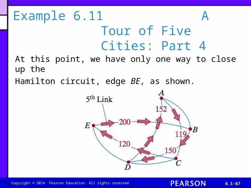
At this point, we have only one way to close up the Hamilton circuit, edge BE, as shown.



The cheapest-link tour shown could have any starting vertex we want. Since Willy lives at A, we describe it as A, C, E, B, D, A. The total cost of this tour is $741, which is a little better than the


nearest-neighbor tour (see Example 6.7) but not as good as the repetitive nearest-neighbor tour (see Example 6.10).


■ Step 1. Pick the cheapest link (i.e., edge with smallest weight) available. (In case of a tie, pick

one at random.) Mark it (say in red).

■ Step 2. Pick the next cheapest link available and

mark it.

ALGORITM 4: THE CHEAPEST LINK ALGORITHM


■ Step 3, 4, …, N – 1. Continue picking and marking

the cheapest unmarked link available that does not

(a) close a circuit or

(b) (b) create three edges coming out of a single vertex

■ Step N. Connect the last two vertices to close the

red circuit. This circuit gives us the cheapest-link tour.

ALGORITM 4: THE CHEAPEST LINK ALGORITHM


The figure shows seven sites on Mars identified as particularly interesting sites for geological exploration.

Example 6.12Roving the Red Planet: Part 2

Our job is to find an optimal tour for a rover that will land at A, visit all the sites to collect rock samples, and at the end return to A.


The distances between sites (in miles) are given in the graph shown.



Let’s look at some of the approaches one might use to tackle this problem.

Brute force: The brute-force algorithm would require us to check and compute 6! = 720 different tours. We will pass on that idea for now.

Cheapest link: The cheapest-link algorithm is a reasonable algorithm to use – not trivial but not too hard either. A summary of the steps is shown in the table on the next slide.



The cheapest-link tour (A, P, W, H, G, N, I, A with a total length of 21,400 miles) is shown.



Here is the cheapest-link tour again (A, P, W, H, G, N, I, A with a total length of 21,400 miles) is shown.



Nearest neighbor: The nearest-neighbor algorithm is the simplest of all the algorithms we learned. Starting from A we go to P, then to W, then to H, then to G, then to I, then to N, and finally back to A. The nearest-neighbor tour (A, P, W, H, G, I, N, A with a total length of 20,100 miles) is shown on the next two slides. (We know that we can repeat this method using different starting points, but we won’t bother with that at this time.)



Nearest neighbor: A, P, W, H, G, I, N, A with a total length of 20,100 miles.



Nearest neighbor:A, P, W, H, G, I, N, A with a total length of 20,100 miles.



The first surprise in Example 6.12 is that the nearest-neighbor algorithm gave us a better tour than the cheapest-link algorithm. Sometimes the cheapest-link algorithm produces a better tour than the nearest-neighbor algorithm, but just as often, it’s the other way around. The two algorithms are different but of equal standing – neither one can be said to be superior to the other one in terms of the quality of the tours it produces.

Surprise One


The second surprise is that the nearest-neighbor tour A, P, W, H, G, I, N, A turns out to be an optimal tour. (This can be verified using a computer and the brute-force algorithm.) Essentially, this means that in this particular example, the simplest of all methods happens to produce the optimal answer–a nice turn of events. Too bad we can’t count on this happening on a more consistent basis!

Surprise Two

Chapter 6: The Mathematics of Touring 6.1 What Is a Traveling Salesman Problem?

Documents

Transcript of Chapter 6: The Mathematics of Touring 6.1 What Is a Traveling Salesman Problem?