Chapter 6 The Integral
82
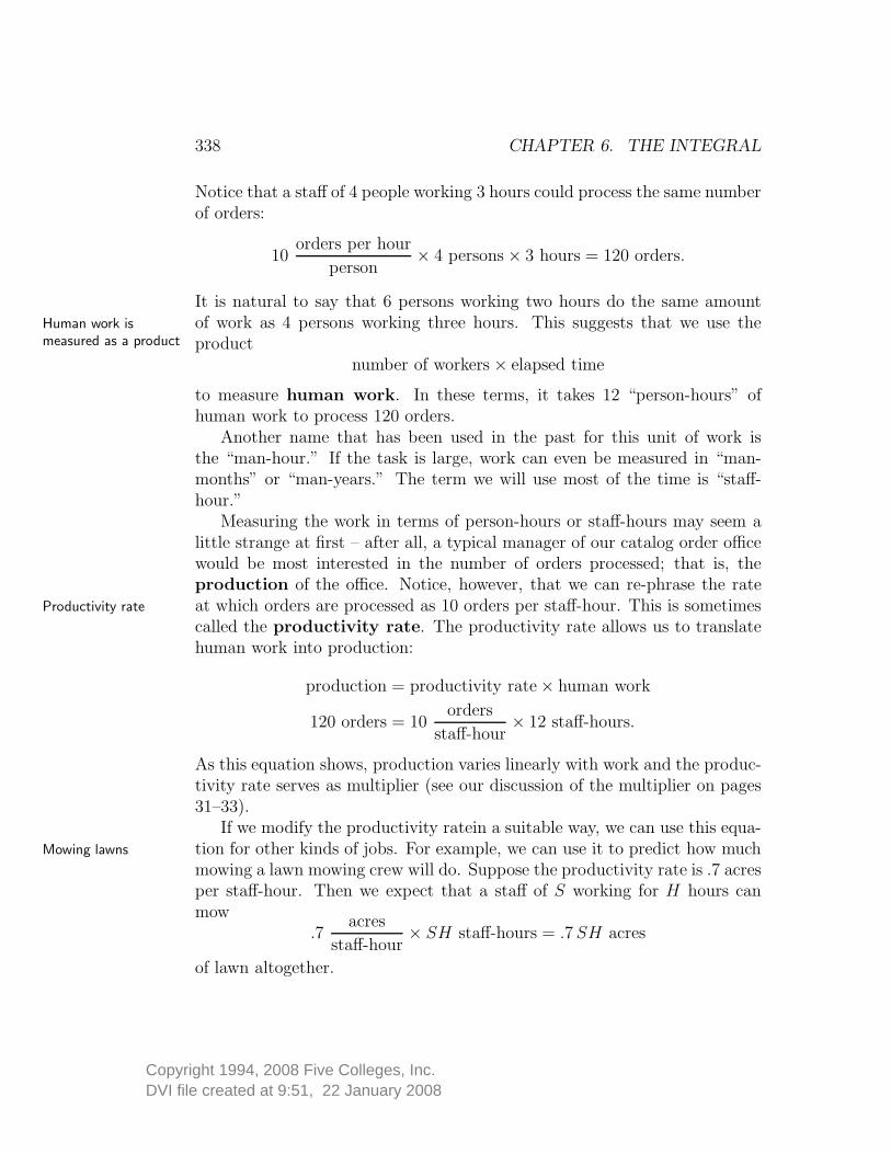
DVI file created at 9:51, 22 January 2008 Copyright 1994, 2008 Five Colleges, Inc. Chapter 6 The Integral There are many contexts—work, energy, area, volume, distance travelled, and profit and loss are just a few—where the quantity in which we are interested is a product of known quantities. For example, the electrical energy needed to burn three 100 watt light bulbs for Δt hours is 300 · Δt watt-hours. In this example, though, the calculation becomes more complicated if lights are turned off and on during the time interval Δt. We face the same complication in any context in which one of the factors in a product varies. To describe such a product we will introduce the integral. As you will see, the integral itself can be viewed as a variable quantity. By analyzing the rate at which that quantity changes, we will find that every integral can be expressed as the solution to a particular differential equation. We will thus be able to use all our tools for solving differential equations to determine integrals. 6.1 Measuring Work Human Work Let’s measure the work done by the staff of an office that processes catalog Processing catalog orders orders. Suppose a typical worker in the office can process 10 orders an hour. Then we would expect 6 people to process 60 orders an hour; in two hours, they could process 120 orders. 10 orders per hour person × 6 persons × 2 hours = 120 orders. 337
Transcript of Chapter 6 The Integral

DVI file created at 9:51, 22 January 2008Copyright 1994, 2008 Five Colleges, Inc.
Chapter 6
The Integral
There are many contexts—work, energy, area, volume, distance travelled, andprofit and loss are just a few—where the quantity in which we are interestedis a product of known quantities. For example, the electrical energy neededto burn three 100 watt light bulbs for ∆t hours is 300 · ∆t watt-hours. Inthis example, though, the calculation becomes more complicated if lights areturned off and on during the time interval ∆t. We face the same complicationin any context in which one of the factors in a product varies. To describesuch a product we will introduce the integral.
As you will see, the integral itself can be viewed as a variable quantity.By analyzing the rate at which that quantity changes, we will find that everyintegral can be expressed as the solution to a particular differential equation.We will thus be able to use all our tools for solving differential equations todetermine integrals.
6.1 Measuring Work
Human Work
Let’s measure the work done by the staff of an office that processes catalog Processingcatalog ordersorders. Suppose a typical worker in the office can process 10 orders an hour.
Then we would expect 6 people to process 60 orders an hour; in two hours,they could process 120 orders.
10orders per hour
person× 6 persons × 2 hours = 120 orders.
337
DVI file created at 9:51, 22 January 2008Copyright 1994, 2008 Five Colleges, Inc.
338 CHAPTER 6. THE INTEGRAL
Notice that a staff of 4 people working 3 hours could process the same numberof orders:
10orders per hour
person× 4 persons × 3 hours = 120 orders.
It is natural to say that 6 persons working two hours do the same amountof work as 4 persons working three hours. This suggests that we use theHuman work is
measured as a product productnumber of workers × elapsed time
to measure human work. In these terms, it takes 12 “person-hours” ofhuman work to process 120 orders.
Another name that has been used in the past for this unit of work isthe “man-hour.” If the task is large, work can even be measured in “man-months” or “man-years.” The term we will use most of the time is “staff-hour.”
Measuring the work in terms of person-hours or staff-hours may seem alittle strange at first – after all, a typical manager of our catalog order officewould be most interested in the number of orders processed; that is, theproduction of the office. Notice, however, that we can re-phrase the rateat which orders are processed as 10 orders per staff-hour. This is sometimesProductivity rate
called the productivity rate. The productivity rate allows us to translatehuman work into production:
production = productivity rate × human work
120 orders = 10orders
staff-hour× 12 staff-hours.
As this equation shows, production varies linearly with work and the produc-tivity rate serves as multiplier (see our discussion of the multiplier on pages31–33).
If we modify the productivity ratein a suitable way, we can use this equa-tion for other kinds of jobs. For example, we can use it to predict how muchMowing lawns
mowing a lawn mowing crew will do. Suppose the productivity rate is .7 acresper staff-hour. Then we expect that a staff of S working for H hours canmow
.7acres
staff-hour× SH staff-hours = .7 SH acres
of lawn altogether.

DVI file created at 9:51, 22 January 2008Copyright 1994, 2008 Five Colleges, Inc.
6.1. MEASURING WORK 339
Production is measured differently in different jobs—as orders processed, Staff-hours provides acommon measure of
work in different jobsor acres mowed, or houses painted. However, in all these jobs human workis measured in the same way, as staff-hours, which gives us a common unitthat can be translated from one job to another.
A staff of S working steadily for H hours does SH staff-hours of work.Suppose, though, the staffing level S is not constant, as in the graph below. Non-constant staffing
Can we still find the total amount of work done?
-
6
0 2 4 6 8 10 120
1
2
3
4
5
time
hours
staff S
2
5
3
pppp
pppppppppppppppppppppppppppppppppp
pppppppppppppppppppppppppppppppppp
pppppppppppppppppppppppp
1.5 5.5 4.0hours hours hours
- � - � -
The basic formula works only when the staffing level is constant. But staffingis constant over certain time intervals. Thus, to find the total amount of workdone, we should simply use the basic formula on each of those intervals, and The work done
is a sum
of productsthen add up the individual contributions. These calculations are done in thefollowing table. The total work is 42.5 staff-hours. So if the productivityrate is 10 orders per staff-hour, 425 orders can be processed.
2 staff ×1.5 hours = 3.0 staff-hours
5 ×5.5 = 27.5
3 ×4.0 = 12.0
total = 42.5 staff-hours
Accumulated work
The last calculation tells us how much work got done over an entire day.What can we tell an office manager who wants to know how work is pro-gressing during the day?
At the beginning of the day, only two people are working, so after thefirst T hours (where 0 ≤ T ≤ 1.5)
work done up to time T = 2 staff × T hours = 2 T staff-hours.

DVI file created at 9:51, 22 January 2008Copyright 1994, 2008 Five Colleges, Inc.
340 CHAPTER 6. THE INTEGRAL
Even before we consider what happens after 1.5 hours, this expression callsour attention to the fact that accumulated work is a function—let’s denoteit W (T ). According to the formula, for the first 1.5 hours W (T ) is a linearfunction whose multiplier is
W ′ = 2staff-hours
hour.
This multiplier is the rate at which work is being accumulated. It is alsoWork accumulates
at a rate equal tothe number of staff
the slope of the graph of W (T ) over the interval 0 ≤ T ≤ 1.5. With thisinsight, we can determine the rest of the graph of W (T ).
What must W (T ) look like on the next time interval 1.5 ≤ T ≤ 7? Here5 members of staff are working, so work is accumulating at the rate of 5staff-hours per hour. Therefore, on this interval the graph of W is a straightline segment whose slope is 5 staff-hours per hour. On the third interval, thegraph is another straight line segment whose slope is 3 staff-hours per hour.The complete graph of W (T ) is shown below.
As the graphs show, the slope of the accumulated work function W (T ) isS is the derivativeof W , so . . . the height of the staffing function S(T ). In other words, S is the derivative
of W :W ′(T ) = S(T ).
-
6
0
1
2
3
4
5
T
hours
staff Sp
p
p
p
p
p
p
p
p
p
p
p
p
p
p
p
p
p
p
p
p
p
p
p
p
p
p
p
p
p
p
p
p
p
p
p
p
p
p
p
p
p
p
p
p
p
p
p
p
p
p
p
p
p
p
p
p
p
p
p
p
p
p
p
p
p
p
p
p
p
p
p
p
p
p
p
p
p
p
p
p
p
p
p
p
p
p
p
p
p
p
p
p
p
2
5
3
-
6
0 2 4 6 8 10 120
10
20
30
40
T
hours
staff-hours W
�������������������
r
r
r
(1.5, 3)
(7, 30.5)
(11, 42.5)
��92
5
3
The accumulated work function W (T )

DVI file created at 9:51, 22 January 2008Copyright 1994, 2008 Five Colleges, Inc.
6.1. MEASURING WORK 341
Notice that the units for W ′ and for S are compatible: the units for W ′ are“staff-hours per hour”, which we can think of as “staff”, the units for S.
We can describe the relation between S and W another way. At themoment, we have explained S in terms of W . However, since we started withS, it is really more appropriate to reverse the roles, and explain W in termsof S. Chapter 4.5 gives us the language to do this: W is an antiderivative . . . W is an
antiderivative of Sof S. In other words, y = W (T ) is a solution to the differential equation
dy
dT= S(T ).
As we find accumulation functions in other contexts, this relation will giveus crucial information.
Before leaving this example we note some special features of S and W .The staffing function S is said to be piecewise constant, or a step func- The derivative of a
piecewise linearfunction
tion. The graphs illustrate the general fact that the derivative of a piecewiselinear function (W , in this case) is piecewise constant.
Summary
The example of human work illustrates the key ideas we will meet, againand again, in different contexts in this chapter. Essentially, we have twofunctions W (t) and S(t) and two different ways of expressing the relationbetween them: On the one hand,
W (t) is an accumulation function for S(t),
while on the other hand,
S(t) is the derivative of W (t).
Exploring the far-reaching implications of functions connected by such a two-fold relationship will occupy the rest of this chapter.

DVI file created at 9:51, 22 January 2008Copyright 1994, 2008 Five Colleges, Inc.
342 CHAPTER 6. THE INTEGRAL
Electrical Energy
Just as humans do work, so does electricity. A power company chargescustomers for the work done by the electricity it supplies, and it measuresthat work in a way that is strictly analogous to the way we measure humanwork. The work done by electricity is usually referred to as (electrical)energy.
For example, suppose we illuminate two light bulbs—one rated at 100watts, the other at 60 watts. It will take the same amount of electricalenergy to burn the 100-watt bulb for 3 hours as it will to burn the 60-wattbulb for 5 hours. Both will use 300 watt-hours of electricity. The powerThe analogy between
electrical energy andhuman work
of the light bulb—measured in watts—is analogous to the number of staffworking (and, in fact, workers have sometimes been called manpower). Thetime the bulb burns is analogous to the time the staff work. Finally, theproduct
energy = power × elapsed time
for electricity is analogous to the product
work = number of staff × elapsed time
for human effort.Electric power is measured in watts, in kilowatts (= 1,000 watts), and in
megawatts (= 1,000,000 watts). Electric energy is measured in watt-hours,in kilowatt-hours (abbreviated ‘kwh’) and in megawatt-hours (abbreviated‘mwh’). Since an individual electrical appliance has a power demand ofabout one kilowatt, kwh are suitable units to use for describing the energyconsumption of a house, while mwh are more natural for a whole town.
Suppose the power demand of a town over a 24 hour period is describedby the following graph:
0 6 12 18 24 hours
time
30
60
90
power
meg
awat
ts

DVI file created at 9:51, 22 January 2008Copyright 1994, 2008 Five Colleges, Inc.
6.1. MEASURING WORK 343
Since this graph decribes power, its vertical height over any point t on the Power is analogous tostaffing leveltime axis tells us the total wattage of the light bulbs, dishwashers, computers,
etc. that are turned on in the town at that instant. This demand fluctuatesbetween 30 and 90 megawatts, roughly. The problem is to determine thetotal amount of energy used in a day—how many megawatt-hours are therein this graph? Although the equation
energy = power × elapsed time,
gives the basic relation between energy and power, we can’t use it directlybecause the power demand isn’t constant.
The staffing function S(t) we considered earlier wasn’t constant, either,but we were still able to compute staff-hours because S(t) was piecewise con-stant. This suggests that we should replace the power graph by a piecewise A piecewise constant
approximationconstant graph that approximates it. Here is one such approximation:
hours
time
30
60
90
power
meg
awat
ts
0 6 9.5 15 21 24
28.5
47
7588
57
As you can see, the step function has five steps, so our approximation tothe total energy consumption of the town will be a sum of five individualproducts:
energy ≈ 28.5 × 6 + 47 × 3.5 + · · · + 57 × 3 = 1447 mwh.
This value is only an estimate, though. How can we get a better estimate?The answer is clear: start with a step function that approximates the powergraph more closely. In principle, we can get as good an approximation as Better estimates
we might desire this way. We are limited only by the precision of the powergraph itself. As our approximation to the power graph improves, so does theaccuracy of the calculation that estimates energy consumption.

DVI file created at 9:51, 22 January 2008Copyright 1994, 2008 Five Colleges, Inc.
344 CHAPTER 6. THE INTEGRAL
In summary, we determine the energy consumption of the town by asequence of successive approximations. The steps in the sequence are listedin the box below.
1. Approximate the power demand by a step function.2. Estimate energy consumption from this approximation.3. Improve the energy estimate by choosing a new step
function that follows power demand more closely.
Accumulated energy consumption
Energy is being consumed steadily over the entire day; can we determinehow much energy has been used through the first T hours of the day? We’llEnergy accumulation
denote this quantity E(T ) and call it the energy accumulation function.For example, we already have the estimate E(24) = 1447 mwh; can weestimate E(3) or E(17.6)?
Once again, the earlier example of human effort can guide us. We sawthat work accumulates at a rate equal to the number of staff present:
W ′(T ) = S(T ).
Since S(T ) was piecewise constant, this rate equation allowed us to determineW (T ) as a piecewise linear function.
We claim that there is an analogous relation between accumulated energyconsumption and power demand—namely
E ′(T ) = p(T ).
Unlike S(T ), the function p(T ) is not piecewise constant. Therefore, theargument we used to show that W ′(T ) = S(T ) will not work here. We needanother argument.
To explain why the differential equation E ′(T ) = p(T ) should be true, wewill start by analyzingEstimating E′(T )
E ′(T ) ≈ ∆E
∆T=
E(T + ∆T ) − E(T )
∆T.
Assume we have made ∆T so small that, to the level of precision we require,the approximation ∆E/∆T agrees with E ′(T ). The numerator ∆E is, by

DVI file created at 9:51, 22 January 2008Copyright 1994, 2008 Five Colleges, Inc.
6.1. MEASURING WORK 345
definition, the total energy used up to time T + ∆T , minus the total energyused up to time T . This is just the energy used during the time interval ∆Tthat runs from time T to time T + ∆T :
∆E = energy used between times T and T + ∆T .
Since the elapsed time ∆T is small, the power demand should be nearlyconstant, so we can get a good estimate for energy consumption from thebasic equation
energy used = power × elapsed time.
In particular, if we represent the power by p(T ), which is the power demandat the beginning of the time period from T to T + ∆T , then we have
∆E ≈ p(T ) · ∆T.
Using this value in our approximation for the derivative E ′(T ), we get
E ′(T ) ≈ ∆E
∆T≈ p(T ) · ∆T
∆T= p(T ).
That is, E ′(T ) ≈ p(T ), and the approximation becomes more and more exactas the time interval ∆T shrinks to 0. Thus,
E ′(T ) = lim∆T→0
∆E
∆T= p(T ).
Here is another way to arrive at the same conclusion. Our starting point A second wayto see that E′ = pis the basic formula
∆E ≈ p(T ) · ∆T,
which holds over a small time interval ∆T . This formula tells us how Eresponds to small changes in T . But that is exactly what the microscopeequation tells us:
∆E ≈ E ′(T ) · ∆T.
Since these equations give the same information, their multipliers must bethe same:
p(T ) = E ′(T ).
In words, the differential equation E ′ = p says that power is the rate at
which energy is consumed. In purely mathematical terms:

DVI file created at 9:51, 22 January 2008Copyright 1994, 2008 Five Colleges, Inc.
346 CHAPTER 6. THE INTEGRAL
The energy accumulation function y = E(t)
is a solution to the differential equation dy/dt = p(t).
In fact, y = E(t) is the solution to the initial value problem
dy
dt= p(t) y(0) = 0.
We can use all the methods described in chapter 4.5 to solve this problem.The relation we have explored between power and energy can be found
in an analogous form in many other contexts, as we will see in the nexttwo sections. In section 4 we will turn back to accumulation functions andinvestigate them as solutions to differential equations. Then, in chapter 11,we will look at some special methods for solving the particular differentialequations that arise in accumulation problems.
Exercises
Human work
1. House-painting is a job that can be done by several people working si-multaneously, so we can measure the amount of work done in “staff-hours.”Consider a house-painting business run by some students. Because of classschedules, different numbers of students will be painting at different timesof the day. Let S(T ) be the number of staff present at time T , measured inhours from 8 am, and suppose that during an 8-hour work day, we have
S(T ) =
3, 0 ≤ T < 2,
2, 2 ≤ T < 4.5,
4, 4.5 ≤ T ≤ 8.
a) Draw the graph of the step function defined here, and compute the totalnumber of staff hours.
b) Draw the graph that shows how staff-hours accumulate on this job. Thisis the graph of the accumulated work function W (T ). (Compare thegraphs of staff and staff-hours on page 340.)
c) Determine the derivative W ′(T ). Is W ′(T ) = S(T )?

DVI file created at 9:51, 22 January 2008Copyright 1994, 2008 Five Colleges, Inc.
6.1. MEASURING WORK 347
2. Suppose that there is a house-painting job to be done, and by past ex-perience the students know that four of them could finish it in 6 hours. Butfor the first 3.5 hours, only two students can show up, and after that, fivewill be available.
a) How long will the whole job take? [Answer: 6.9 hours.]
b) Draw a graph of the staffing function for this problem. Mark on thegraph the time that the job is finished.
c) Draw the graph of the accumulated work function W (T ).
d) Determine the derivative W ′(T ). Is W ′(T ) = S(T )?
Average staffing. Suppose a job can be done in three hours when 6 peoplework the first hour and 9 work during the last two hours. Then the job takes24 staff-hours of work, and the average staffing is
average staffing =24 staff-hours
3 hours= 8 staff.
This means that a constant staffing level of 8 persons can accomplish thejob in the same time that the given variable staffing level did. Note that theaverage staffing level (8 persons) is not the average of the two numbers 9 and6!
3. What is the average staffing of the jobs considered in exercises 1 and 2,above?
4. a) Draw the graph that shows how work would accumulate in the jobdescribed in exercise 1 if the work-force was kept at the average staffing levelinstead of the varying level described in the exercise. Compare this graph tothe graph you drew in exercise 1 b.
b) What is the derivative W ′(T ) of the work accumulation function whosegraph you drew in part (a)?
5. What is the average staffing for the job described by the graph onpage 339?
Electrical energy
6. On Monday evening, a 1500 watt space heater is left on from 7 until 11pm. How many kilowatt-hours of electricity does it consume?

DVI file created at 9:51, 22 January 2008Copyright 1994, 2008 Five Colleges, Inc.
348 CHAPTER 6. THE INTEGRAL
7. a) That same heater also has settings for 500 and 1000 watts. Supposethat on Tuesday we put it on the 1000 watt setting from 6 to 8 pm, thenswitch to 1500 watts from 8 till 11 pm, and then on the 500 watt settingthrough the night until 8 am, Wednesday. How much energy is consumed (inkwh)?
b) Sketch the graphs of power demand p(T ) and accumulated energy con-sumption E(T ) for the space heater from Tuesday evening to Wednesdaymorning. Determine whether E ′(T ) = p(T ) in this case.
c) The average power demand of the space heater is defined by:
average power demand =energy consumption
elapsed time.
If energy consumption is measured in kilowatt-hours, and time in hours, thenwe can measure average power demand in kilowatts—the same as poweritself. (Notice the similarity with average staffing.) What is the averagepower demand from Tuesday evening to Wednesday morning? If the heatercould be set at this average power level, how would the energy consumptioncompare to the actual energy consumption you determined in part (a)?
8. The graphs on pages 342 and 343 describe the power demand of a townover a 24-hour period. Give an estimate of the average power demand of thetown during that period. Explain what you did to produce your estimate.[Answer: 60.29 megawatts is one estimate.]
Work as force × distance
The effort it takes to move an object is also called work. Since it takes twice
as much effort to move the object twice as far, or to move another objectthat is twice as heavy, we can see that the work done in moving an objectis proportional to both the force applied and to the distance moved. Thesimplest way to express this fact is to define
work = force × distance.
For example, to lift a weight of 20 pounds straight up it takes 20 pounds offorce. If the vertical distance is 3 feet then
20 pounds × 3 feet = 60 foot-pounds

DVI file created at 9:51, 22 January 2008Copyright 1994, 2008 Five Colleges, Inc.
6.1. MEASURING WORK 349
of work is done. Thus, once again the quantity we are interested in has theform of a product. The foot-pound is one of the standard units for measuringwork.
9. Suppose a tractor pulls a loaded wagon over a road whose steepnessvaries. If the first 150 feet of road are relatively level and the tractor has toexert only 200 pounds of force while the next 400 feet are inclined and thetractor has to exert 550 pounds of force, how much work does the tractor doaltogether?
10. A motor on a large ship is lifting a 2000 pound anchor that is alreadyout of the water at the end of a 30 foot chain. The chain weighs 40 poundsper foot. As the motor lifts the anchor, the part of the chain that is hanginggets shorter and shorter, thereby reducing the weight the motor must lift.
a) What is the combined weight of anchor and hanging chain when theanchor has been lifted x feet above its initial position?
b) Divide the 30-foot distance that the anchor must move into 3 equal in-tervals of 10 feet each. Estimate how much work the motor does lifting theanchor and chain over each 10-foot interval by multiplying the combinedweight at the bottom of the interval by the 10-foot height. What is your es-timate for the total work done by the motor in raising the anchor and chain30 feet?
c) Repeat all the steps of part (b), but this time use 30 equal intervals of1 foot each. Is your new estimate of the work done larger or smaller thanyour estimate in part (b)? Which estimate is likely to be more accurate? Onwhat do you base your judgment?
d) If you ignore the weight of the chain entirely, what is your estimate ofthe work done? How much extra work do you therefore estimate the motormust do to raise the heavy chain along with the anchor?
DVI file created at 9:51, 22 January 2008Copyright 1994, 2008 Five Colleges, Inc.
350 CHAPTER 6. THE INTEGRAL
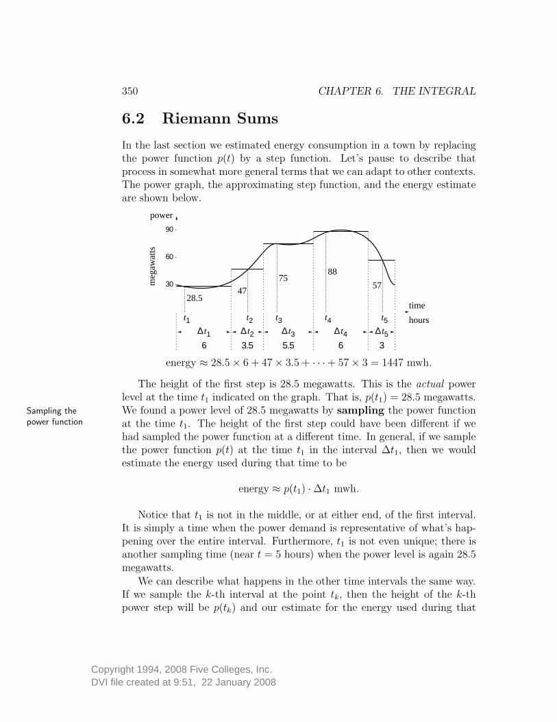
6.2 Riemann Sums
In the last section we estimated energy consumption in a town by replacingthe power function p(t) by a step function. Let’s pause to describe thatprocess in somewhat more general terms that we can adapt to other contexts.The power graph, the approximating step function, and the energy estimateare shown below.
hours
time
30
60
90
power
meg
awat
ts
t1 t2 t3 t4 t5
28.547
7588
57
∆ t1 ∆ t2 ∆ t3 ∆ t4 ∆ t56 3.5 5.5 6 3
energy ≈ 28.5 × 6 + 47 × 3.5 + · · ·+ 57 × 3 = 1447 mwh.
The height of the first step is 28.5 megawatts. This is the actual powerlevel at the time t1 indicated on the graph. That is, p(t1) = 28.5 megawatts.We found a power level of 28.5 megawatts by sampling the power functionSampling the
power function at the time t1. The height of the first step could have been different if wehad sampled the power function at a different time. In general, if we samplethe power function p(t) at the time t1 in the interval ∆t1, then we wouldestimate the energy used during that time to be
energy ≈ p(t1) · ∆t1 mwh.
Notice that t1 is not in the middle, or at either end, of the first interval.It is simply a time when the power demand is representative of what’s hap-pening over the entire interval. Furthermore, t1 is not even unique; there isanother sampling time (near t = 5 hours) when the power level is again 28.5megawatts.
We can describe what happens in the other time intervals the same way.If we sample the k-th interval at the point tk, then the height of the k-thpower step will be p(tk) and our estimate for the energy used during that

DVI file created at 9:51, 22 January 2008Copyright 1994, 2008 Five Colleges, Inc.
6.2. RIEMANN SUMS 351
time will beenergy ≈ p(tk) · ∆tk mwh.
We now have a general way to construct an approximation for the power A procedure forapproximating powerlevel and energy use
function and an estimate for the energy consumed over a 24-hour period. Itinvolves these steps.
1. Choose any number n of subintervals, and let them have arbitrarypositive widths ∆t1, ∆t2, . . . , ∆tn, subject only to the condition
∆t1 + · · · + ∆tn = 24 hours.
2. Sample the k-th subinterval at any point tk, and let p(tk) represent thepower level over this subinterval.
3. Estimate the energy used over the 24 hours by the sum
energy ≈ p(t1) · ∆t1 + p(t2) · ∆t2 + · · ·+ p(tn) · ∆tn mwh.
The expression on the right is called a Riemann sum for the power functionp(t) on the interval 0 ≤ t ≤ 24 hours.
The work of Bernhard Riemann (1826–1866) has had a profound influence on contemporarymathematicians and physicists. His revolutionary ideas about the geometry of space, for example,are the basis for Einstein’s theory of general relativity.
The enormous range of choices in this process means there are innu-merable ways to construct a Riemann sum for p(t). However, we are notreally interested in arbitrary Riemanns sums. On the contrary, we want to Choices that lead
to good estimatesbuild Riemann sums that will give us good estimates for energy consump-tion. Therefore, we will choose each subinterval ∆tk so small that the powerdemand over that subinterval differs only very little from the sampled valuep(tk). A Riemann sum constructed with these choices will then differ onlyvery little from the total energy used during the 24-hour time interval.
Essentially, we use a Riemann sum to resolve a dilemma. We know thebasic formula
energy = power × time
works when power is constant, but in general power isn’t constant—that’sthe dilemma. We resolve the dilemma by using instead a sum of terms of The dilemma
the form power × time . With this sum we get an estimate for the energy.

DVI file created at 9:51, 22 January 2008Copyright 1994, 2008 Five Colleges, Inc.
352 CHAPTER 6. THE INTEGRAL
In this section we will explore some other problems that present the samedilemma. In each case we will start with a basic formula that involves aproduct of two constant factors, and we will need to adapt the formula tothe situation where one of the factors varies. The solution will be to constructa Riemann sum of such products, producing an estimate for the quantity wewere after in the first place. As we work through each of these problems, youshould pause to compare it to the problem of energy consumption.
Calculating Distance Travelled
It is easy to tell how far a car has travelled by reading its odometer. Theproblem is more complicated for a ship, particularly a sailing ship in the daysbefore electronic navigation was common. The crew always had instrumentsEstimating velocity
and distance that could measure—or at least estimate—the velocity of the ship at anytime. Then, during any time interval in which the ship’s velocity is constant,the distance travelled is given by the familiar formula
distance = velocity × elapsed time.
If the velocity is not constant, then this formula does not work. Theremedy is to break up the long time period into several short ones. Supposetheir lengths are ∆t1, ∆t2, . . . , ∆tn. By assumption, the velocity is a functionof time t; let’s denote it v(t). At some time tk during each time period ∆tkSampling the
velocity function measure the velocity: vk = v(tk). Then the Riemann sum
v(t1) · ∆t1 + v(t2) · ∆t2 + · · ·+ v(tn) · ∆tn
is an estimate for the total distance travelled.For example, suppose the velocity is measured five times during a 15 hour
trip—once every three hours—as shown in the table below. Then the basicformula
distance = velocity × elapsed time.
gives us an estimate for the distance travelled during each three-hour period,and the sum of these distances is an estimate of the total distance travelledduring the fifteen hours. These calculations appear in the right-hand columnof the table. (Note that the first measurement is used to calculate the distancetravelled between hours 0 and 3, while the last measurement, taken 12 hoursafter the start, is used to calculate the distance travelled between hours 12and 15.)

DVI file created at 9:51, 22 January 2008Copyright 1994, 2008 Five Colleges, Inc.
6.2. RIEMANN SUMS 353
sampling elapsedtime time velocity distance travelled
(hours) (hours) (miles/hour) (miles)
0369
12
33333
1.45.254.34.65.0
3 × 1.4 = 4.203 × 5.25 = 15.753 × 4.3 = 12.903 × 4.6 = 13.803 × 5.0 = 15.00
61.65
Thus we estimate the ship has travelled 61.65 miles during the fifteen hours. The estimated distanceis a Riemann sum forthe velocity function
The number 61.65, obtained by adding the numbers in the right-most column,is a Riemann sum for the velocity function.
Consider the specific choices that we made to construct this Riemannsum:
∆t1 = ∆t2 = ∆t3 = ∆t4 = ∆t5 = 3
t1 = 0, t2 = 3, t3 = 6, t4 = 9, t5 = 12.
These choices differ from the choices we made in the energy example intwo notable ways. First, all the subintervals here are the same size. This Intervals and sampling
times are chosen ina systematic way
is because it is natural to take velocity readings at regular time intervals.By contrast, in the energy example the subintervals were of different widths.Those widths were chosen in order to make a piecewise constont function thatfollowed the power demand graph closely. Second, all the sampling times lieat the beginning of the subintervals in which they appear. Again, this isnatural and convenient for velocity measurements. In the energy example,the sampling times were chosen with an eye to the power graph. Even thoughwe can make arbitrary choices in constructing a Riemann sum, we will do itsystematically whenever possible. This means choosing subintervals of equalsize and sampling points at the “same” place within each interval.
Let’s turn back to our estimate for the total distance. Since the velocityof the ship could have fluctuated significantly during each of the three-hourperiods we used, our estimate is rather rough. To improve the estimate we Improving the
distance estimatecould measure the velocity more frequently—for example, every 15 minutes.If we did, the Riemann sum would have 60 terms (four distances per hourfor 15 hours). The individual terms in the sum would all be much smaller,though, because they would be estimates for the distance travelled in 15

DVI file created at 9:51, 22 January 2008Copyright 1994, 2008 Five Colleges, Inc.
354 CHAPTER 6. THE INTEGRAL
minutes instead of in 3 hours. For instance, the first of the 60 terms wouldbe
1.4miles
hour× .25 hours = .35 miles.
Of course it may not make practical sense to do such a precise calculation.Other factors, such as water currents or the inaccuracy of the velocity mea-surements themselves, may keep us from getting a good estimate for thedistance. Essentially, the Riemann sum is only a model for the distancecovered by a ship.
Calculating Areas
The area of a rectangle is just the product of itslength and its width. How can we measure thearea of a region that has an irregular boundary,like the one at the left? We would like to use thebasic formula
area = length × width.
However, since the region doesn’t have straightsides, there is nothing we can call a “length” or a“width” to work with.
We can begin to deal with this problem bybreaking up the region into smaller regions thatdo have straight sides—with, at most, only onecurved side. This can be done many differentways. The lower figure shows one possibility. Thesum of the areas of all the little regions will bethe area we are looking for. Although we haven’tyet solved the original problem, we have at leastreduced it to another problem that looks simplerand may be easier to solve. Let’s now work on thereduced problem for the shaded region.

DVI file created at 9:51, 22 January 2008Copyright 1994, 2008 Five Colleges, Inc.
6.2. RIEMANN SUMS 355
Here is the shaded region, turned so that it sitsflat on one of its straight sides. We would like tocalculate its area using the formula
width × height,
but this formula applies only to rectangles. Wecan, however, approximate the region by a col-lection of rectangles, as shown at the right. Theformula does apply to the individual rectanglesand the sum of their areas will approximate thearea of the whole region.
To get the area of a rectangle, we must measureits width and height. Their heights vary with theheight of the curved top of the shaded region. Todescribe that height in a systematic way, we haveplaced the shaded region in a coordinate plane sothat it sits on the x-axis. The other two straightsides lie on the vertical lines x = a and x = b.
a x b x
y
f(x)
The curved side defines the graph of a function y = f(x). Therefore, ateach point x, the vertical height from the axis to the curve is f(x). Byintroducing a coordinate plane we gain access to mathematical tools—suchas the language of functions—to describe the various areas.
The k-th rectangle has been singled out on the left, below. We let ∆xk Calculating the areasof the rectanglesdenote the width of its base. By sampling the function f at a properly
chosen point xk in the base, we get the height f(xk) of the rectangle. Itsarea is therefore f(xk) · ∆xk. If we do the same thing for all n rectanglesshown on the right, we can write their total area as
f(x1) · ∆x1 + f(x2) · ∆x2 + · · ·+ f(xn) · ∆xn.
a b x
y
f(xk)
xk
∆xk
a b x
y

DVI file created at 9:51, 22 January 2008Copyright 1994, 2008 Five Colleges, Inc.
356 CHAPTER 6. THE INTEGRAL
Notice that our estimate for the area has the form of a Riemann sumThe area estimate isa Riemann sum for the height function f(x) over the interval a ≤ x ≤ b. To get a better
estimate, we should use narrower rectangles, and more of them. In otherwords, we should construct another Riemann sum in which the number ofterms, n, is larger and the width ∆xk of every subinterval is smaller. Puttingit yet another way, we should sample the height more often.
Consider what happens if we apply this procedure to a region whose areawe know already. The semicircle of radius r = 1 has an area of πr2/2 =π/2 = 1.5707963 . . . . The semicircle is the graph of the function
f(x) =√
1 − x2,
which lies over the interval −1 ≤ x ≤ 1. To get the figure on the left, wesampled the height f(x) at 20 evenly spaced points, starting with x = −1.In the better approximation on the right, we increased the number of samplepoints to 50. The values of the shaded areas were calculated with the programRIEMANN, which we will develop later in this section. Note that with 50rectangles the Riemann sum is within .005 of π/2, the exact value of thearea.
x
y
-1 1
shaded area = 1.552259
x
y
-1 1
shaded area = 1.566098
Calculating Lengths
It is to be expected that products—and ultimately, Riemann sums—will beinvolved in calculating areas. It is more surprising to find that we can usethem to calculate lengths, too. In fact, when we are working in a coordinateplane, using a product to describe the length of a straight line is even quitenatural.

DVI file created at 9:51, 22 January 2008Copyright 1994, 2008 Five Colleges, Inc.
6.2. RIEMANN SUMS 357
To see how this can happen, consider a line segment in the x, y-plane The length ofa straight linethat has a known slope m. If we also know the horizontal separation between
the two ends, we can find the length of the seg-ment. Suppose the horizontal separation is ∆x andthe vertical separation ∆y. Then the length of thesegment is √
∆x2 + ∆y2
������������
m
∆x� -pppppppppppppppppppppppppp
pppppppppppppppppppppppppp
by the Pythagorean theorem (see page 90). Since ∆y = m · ∆x, we canrewrite this as √
∆x2 + (m · ∆x)2 = ∆x ·√
1 + m2.
In other words, if a line has slope m and it is ∆x units wide, then its lengthis the product √
1 + m2 · ∆x.
Suppose the line is curved, instead of straight. Can we describe its length The length ofa curved linethe same way? We’ll assume that the curve is the graph y = g(x). The
complication is that the slope m = g′(x) now varies with x.If g′(x) doesn’t vary too much over an interval oflength ∆x, then the curve is nearly straight. Picka point x∗ in that interval and sample the slopeg′(x∗) there; we expect the length of the curve tobe approximately
√
1 + (g′(x∗))2 · ∆x.
������������g′(x∗) x∗
r
∆x� -pppppppppppppppppppppppppppppppppppp
pppppppppppppppppppppppppppppppppppp
As the figure shows, this is the exact length of the straight line segment thatlies over the same interval ∆x and is tangent to the curve at the point x = x∗.
If the slope g′(x) varies appreciably over the interval, we should subdividethe interval into small pieces ∆x1, ∆x2, . . . , ∆xn, over which the curve isnearly straight. Then, if we sample the slope at the point xk in the k-thsubinterval, the sum
√
1 + (g′(x1))2 · ∆x1 + · · · +√
1 + (g′(xn))2 · ∆xn
will give us an estimate for the total length of the curve.

DVI file created at 9:51, 22 January 2008Copyright 1994, 2008 Five Colleges, Inc.
358 CHAPTER 6. THE INTEGRAL
Once again, we find an expression that has the form of a Riemann sum.The length of a curveis estimated bya Riemann sum
There is, however, a new ingredient worth noting. The estimate is a Riemannsum not for the original function g(x) but for another function
f(x) =√
1 + (g′(x))2
that we constructed using g. The important thing is that the length isestimated by a Riemann sum for some function.
x
y
π4-segment length = 3.8199
x
y
π20-segment length = 3.8202
The figure above shows two estimates for the length of the graph of y =sin x between 0 and π. In each case, we used subintervals of equal length andwe sampled the slope at the left end of each subinterval. As you can see, thefour segments approximate the graph of y = sin x only very roughly. Whenwe increase the number of segments to 20, on the right, the approximationto the shape of the graph becomes quite good. Notice that the graph itselfis not shown on the right; only the 20 segments.
To calculate the two lengths, we constructed Riemann sums for the func-tion f(x) =
√1 + cos2 x. We used the fact that the derivative of g(x) = sin x
is g′(x) = cos x, and we did the calculations using the program RIEMANN.By using the program with still smaller subintervals you can show that
the exact length = 3.820197789 . . . .
Thus, the 20-segment estimate is already accurate to four decimal places.
We have already constructed estimates for the length of a curve, in chapter 2 (pages 89–91).Those estimates were sums, too, but they were not Riemann sums. The terms had the form√
∆x2 + ∆y2; they were not products of the form√
1 + m2 · ∆x. The sums in chapter 2 mayseem more straightforward. However, we are developing Riemann sums as a powerful generaltool for dealing with many different questions. By expressing lengths as Riemann sums we gainaccess to that power.
DVI file created at 9:51, 22 January 2008Copyright 1994, 2008 Five Colleges, Inc.
6.2. RIEMANN SUMS 359
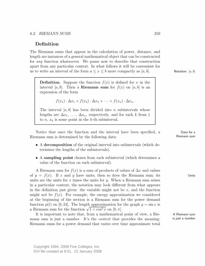
Definition
The Riemann sums that appear in the calculation of power, distance, andlength are instances of a general mathematical object that can be constructedfor any function whatsoever. We pause now to describe that constructionapart from any particular context. In what follows it will be convenient forus to write an interval of the form a ≤ x ≤ b more compactly as [a, b]. Notation: [a, b]
Definition. Suppose the function f(x) is defined for x in theinterval [a, b]. Then a Riemann sum for f(x) on [a, b] is anexpression of the form
f(x1) · ∆x1 + f(x2) · ∆x2 + · · ·+ f(xn) · ∆xn.
The interval [a, b] has been divided into n subintervals whoselengths are ∆x1, . . . , ∆xn, respectively, and for each k from 1to n, xk is some point in the k-th subinterval.
Notice that once the function and the interval have been specified, a Data for aRiemann sumRiemann sum is determined by the following data:
• A decomposition of the original interval into subintervals (which de-termines the lengths of the subintervals).
• A sampling point chosen from each subinterval (which determines avalue of the function on each subinterval).
A Riemann sum for f(x) is a sum of products of values of ∆x and valuesof y = f(x). If x and y have units, then so does the Riemann sum; its Units
units are the units for x times the units for y. When a Riemann sum arisesin a particular context, the notation may look different from what appearsin the definition just given: the variable might not be x, and the functionmight not be f(x). For example, the energy approximation we consideredat the beginning of the section is a Riemann sum for the power demandfunction p(t) on [0, 24]. The length approximation for the graph y = sin x isa Riemann sum for the function
√1 + cos2 x on [0, π].
It is important to note that, from a mathematical point of view, a Rie- A Riemann sumis just a numbermann sum is just a number. It’s the context that provides the meaning:
Riemann sums for a power demand that varies over time approximate total

DVI file created at 9:51, 22 January 2008Copyright 1994, 2008 Five Colleges, Inc.
360 CHAPTER 6. THE INTEGRAL
energy consumption; Riemann sums for a velocity that varies over time ap-proximate total distance; and Riemann sums for a height that varies overdistance approximate total area.
To illustrate the generality of a Riemann sum, and to stress that it isjust a number arrived at through arbitrary choices, let’s work through anexample without a context. Consider the function
f(x) =√
1 + x3 on [1, 3].
We will break up the full interval [1, 3] into three subintervals [1, 1.6], [1.6, 2.3]The data
and [2.3, 3]. Thus∆x1 = .6 ∆x2 = ∆x3 = .7.
Next we’ll pick a point in each subinterval, say x1 = 1.3, x2 = 2 and x3 = 2.8.Here is the data laid out on the x-axis.
--� -� -�
∆x1 = .6 ∆x2 = .7 ∆x2 = .7
1 1.6 2.3 3
r r r
1.3 2 2.8 x
With this data we get the following Riemann sum for√
1 + x3 on [1, 3]:
f(x1) · ∆x1 + f(x2) · ∆x2 + f(x3) · ∆x3
=√
1 + 1.33 × .6 +√
1 + 23 × .7 +√
1 + 2.83 × .7
= 6.5263866
In this case, the choice of the subintervals, as well as the choice of the point xk
in each subinterval, was haphazard. Different data would produce a differentvalue for the Riemann sum.
Keep in mind that an individual Riemann sum is not especially significant.Ultimately, we are interested in seeing what happens when we recalculateRiemann sums with smaller and smaller subintervals. For that reason, it ishelpful to do the calculations systematically.
Calculating a Riemann sum algorithmically. As we have seen with ourSystematic data
contextual problems, the data for a Riemann sum is not usually chosen in ahaphazard fashion. In fact, when dealing with functions given by formulas,such as the function f(x) =
√1 − x2 whose graph is a semicircle, it pays to
be systematic. We use subintervals of equal size and pick the “same” point

DVI file created at 9:51, 22 January 2008Copyright 1994, 2008 Five Colleges, Inc.
6.2. RIEMANN SUMS 361
from each subinterval (e.g., always pick the midpoint or always pick the leftendpoint). The benefit of systematic choices is that we can write down thecomputations involved in a Riemann sum in a simple algorithmic form thatcan be carried out on a computer.
Let’s illustrate how this strategy applies to the function√
1 + x3 on [1, 3].Since the whole interval is 3−1 = 2 units long, if we construct n subintervalsof equal length ∆x, then ∆x = 2/n. For every k = 1, . . . , n, we choose thesampling point xk to be the left endpoint of the k-th subinterval. Here is apicture of the data:
. . . -r r r r r r
-� -� -� -�∆x ∆x ∆x ∆x
3x1 x2 x3 xn
6 6 6 61 1 + ∆x 1 + 2∆x 1 + (n − 1)∆x
x
In this systematic approach, the space between one sampling point and thenext is ∆x, the same as the width of a subinterval. This puts the k-thsampling point at x = 1 + (k − 1)∆x.
In the following table, we add up the terms in a Riemann sum S forf(x) =
√1 + x3 on the interval [1, 3]. We used n = 4 subintervals and
always sampled f at the left endpoint. Each row shows the following:
1. the current sampling point;
2. the value of f at that point;
3. the current term ∆S = f · ∆x in the sum;
4. the accumulated value of S.
left current current accumulatedendpoint
√1 + x3 ∆S S
11.522.5
1.41422.091734.0774
.70711.04581.52.0387
.70711.75293.25295.2916
The Riemann sum S appears as the final value 5.2916 in the fourth column.
The program RIEMANN, below, will generate the last two columns in theabove table. The statement x = a on the sixth line determines the position

DVI file created at 9:51, 22 January 2008Copyright 1994, 2008 Five Colleges, Inc.
362 CHAPTER 6. THE INTEGRAL
of the first sampling point. Within the FOR–NEXT loop, the statement x
= x + deltax moves the sampling point to its next position.
Program: RIEMANNLeft endpoint Riemann sums
DEF fnf (x) = SQR(1 + x ^ 3)
a = 1
b = 3
numberofsteps = 4
deltax = (b - a) / numberofsteps
x = a
accumulation = 0
FOR k = 1 TO numberofsteps
deltaS = fnf(x) * deltax
accumulation = accumulation + deltaS
x = x + deltax
PRINT deltaS, accumulation
NEXT k
By modifying RIEMANN, you can calculate Riemann sums for other sam-pling points and for other functions. For example, to sample at midpoints,you must start at the midpoint of the first subinterval. Since the subintervalis ∆x units wide, its midpoint is ∆x/2 units from the left endpoint, which isx = a. Thus, to have the program generate midpoint sums, just change thestatement that “initializes” x (line 6) to x = a + deltax / 2.
Summation Notation
Because Riemann sums arise frequently and because they are unwieldy towrite out in full, we now introduce a method—called summation notation—that allows us to write them more compactly. To see how it works, look firstat the sum
12 + 22 + 32 + · · ·+ 502.
Using summation notation, we can express this as
50∑
k=1
k2.

DVI file created at 9:51, 22 January 2008Copyright 1994, 2008 Five Colleges, Inc.
6.2. RIEMANN SUMS 363
For a somewhat more abstract example, consider the sum
a1 + a2 + a3 + · · · + an,
which we can express asn∑
k=1
ak.
We use the capital letter sigma∑
from the Greek alphabet to denote asum. For this reason, summation notation is sometimes referred to as sigmanotation. You should regard
∑as an instruction telling you to sum the Sigma notation
numbers of the indicated form as the index k runs through the integers,starting at the integer displayed below the
∑and ending at the integer
displayed above it. Notice that changing the index k to some other letter hasno effect on the sum. For example,
20∑
k=1
k3 =20∑
j=1
j3,
since both expressions give the sum of the cubes of the first twenty posi-tive integers. Other aspects of summation notation will be covered in theexercises.
Summation notation allows us to write the Riemann sum
f(x1) · ∆x1 + · · · + f(xn) · ∆xn
more efficiently asn∑
k=1
f(xk) · ∆xk.
Be sure not to get tied into one particular way of using these symbols. Forexample, you should instantly recognize
m∑
i=1
∆ti g(ti)
as a Riemann sum. In what follows we will commonly use summation nota-tion when working with Riemann sums. The important thing to rememberis that summation notation is only a “shorthand” to express a Riemann sumin a more compact form.

DVI file created at 9:51, 22 January 2008Copyright 1994, 2008 Five Colleges, Inc.
364 CHAPTER 6. THE INTEGRAL
Exercises
Making approximations
1. Estimate the average velocity of the ship whose motion is described onpage 352. The voyage lasts 15 hours.
2. The aim of this question is to determine how much electrical energy wasconsumed in a house over a 24-hour period, when the power demand p wasmeasured at different times to have these values:
time power(24-hour clock) (watts)
1:305:008:009:30
11:0015:0018:3020:0022:3023:00
275240730300150225
1880950700350
Notice that the time interval is from t = 0 hours to t = 24 hours, but thepower demand was not sampled at either of those times.
a) Set up an estimate for the energy consumption in the form of a Riemannsum p(t1)∆t1 + · · · + p(tn)∆tn for the power function p(t). To do this, youmust identify explicitly the value of n, the sampling times tk, and the timeintervals ∆tk that you used in constructing your estimate. [Note: the sam-pling times come from the table, but there is wide latitude in how you choosethe subintervals ∆tk.]
b) What is the estimated energy consumption, using your choice of data?There is no single “correct” answer to this question. Your estimate dependson the choices you made in setting up the Riemann sum.
c) Plot the data given in the table in part (a) on a (t, p)-coordinate plane.Then draw on the same coordinate plane the step function that representsyour estimate of the power function p(t). The width of the k-th step shouldbe the time interval ∆tk that you specified in part (a); is it?

DVI file created at 9:51, 22 January 2008Copyright 1994, 2008 Five Colleges, Inc.
6.2. RIEMANN SUMS 365
d) Estimate the average power demand in the house during the 24-hourperiod.
Waste production. A colony of living yeast cells in a vat of fermentinggrape juice produces waste products—mainly alcohol and carbon dioxide—as it consumes the sugar in the grape juice. It is reasonable to expect thatanother yeast colony, twice as large as this one, would produce twice as muchwaste over the same time period. Moreover, since waste accumulates overtime, if we double the time period we would expect our colony to producetwice as much waste.
These observations suggest that waste production is proportional to boththe size of the colony and the amount of time that passes. If P is the sizeof the colony, in grams, and ∆t is a short time interval, then we can expresswaste production W as a function of P and ∆t:
W = k · P · ∆t grams.
If ∆t is measured in hours, then the multiplier k has to be measured in unitsof grams of waste per hour per gram of yeast.
The preceding formula is useful only over a time interval ∆t in which thepopulation size P does not vary significantly. If the time interval is large, andthe population size can be expressed as a function P (t) of the time t, then wecan estimate waste production by breaking up the whole time interval intoa succession of smaller intervals ∆t1, ∆t2, . . . , ∆tn and forming a Riemannsum
k P (t1) ∆t1 + · · ·+ k P (tn) ∆tn ≈ W grams.
The time tk must lie within the time interval ∆tk, and P (tk) must be a goodapproximation to the population size P (t) throughout that time interval.
3. Suppose the colony starts with 300 grams of yeast (i.e., at time t = 0hours) and it grows exponentially according to the formula
P (t) = 300 e0.2 t .
If the waste production constant k is 0.1 grams per hour per gram of yeast,estimate how much waste is produced in the first four hours. Use a Riemannsum with four hour-long time intervals and measure the population size ofthe yeast in the middle of each interval—that is, “on the half-hour.”

DVI file created at 9:51, 22 January 2008Copyright 1994, 2008 Five Colleges, Inc.
366 CHAPTER 6. THE INTEGRAL
Using RIEMANN
4. a) Calculate left endpoint Riemann sums for the function√
1 + x3 onthe interval [1, 3] using 40, 400, 4000, and 40000 equally-spaced subintervals.How many ddecimal points in this sequence have stabilized?
b) The left endpoint Riemann sums for√
1 + x3 on the interval [1, 3] seemto be approaching a limit as the number of subintervals increases withoutbound. Give the numerical value of that limit, accurate to four decimalplaces.
c) Calculate left endpoint Riemann sums for the function√
1 + x3 on theinterval [3, 7]. Construct a sequence of Riemann sums using more and moresubintervals, until you can determine the limiting value of these sums, accu-rate to three decimal places. What is that limit?
d) Calculate left endpoint Riemann sums for the function√
1 + x3 on theinterval [1, 7] in order to determine the limiting value of the sums to threedecimal place accuracy. What is that value? How are the limiting values inparts (b), (c), and (d) related? How are the corresponding intervals related?
5. Modify RIEMANN so it will calculate a Riemann sum by sampling thegiven function at the midpoint of each subinterval, instead of the left end-point. Describe exactly how you changed the program to do this.
6. a) Calculate midpoint Riemann sums for the function√
1 + x3 on theinterval [1, 3] using 40, 400, 4000, and 40000 equally-spaced subintervals.How many decimal points in this sequence have stabilized?
b) Roughly how many subintervals are needed to make the midpoint Rie-mann sums for
√1 + x3 on the interval [1, 3] stabilize out to the first four
digits? What is the stable value? Compare this to the limiting value youfound earlier for left endpoint Riemann sums. Is one value larger than theother; could they be the same?
c) Comment on the relative “efficiency” of midpoint Riemann sums versusleft endpoint Riemann sums (at least for the function
√1 + x3 on the interval
[1, 3]). To get the same level of accuracy, an efficient calculation will takefewer steps than an inefficient one.
7. a) Modify RIEMANN to calculate right endpoint Riemann sums, anduse it to calculate right endpoint Riemann sums for the function
√1 + x3 on

DVI file created at 9:51, 22 January 2008Copyright 1994, 2008 Five Colleges, Inc.
6.2. RIEMANN SUMS 367
the interval [1, 3] using 40, 400, 4000, and 40000 equally-spaced subintervals.How many digits in this sequence have stabilized?
b) Comment on the efficiency of right endpoint Riemann sums as comparedto left endpoint and to midpoint Riemann sums—at least as far as the func-tion
√1 + x3 is concerned.
8. Calculate left endpoint Riemann sums for the function
f(x) =√
1 − x2 on the interval [−1, 1].
Use 20 and 50 equally-spaced subintervals. Compare your values with theestimates for the area of a semicircle given on page 356.
9. a) Calculate left endpoint Riemann sums for the function
f(x) =√
1 + cos2 x on the interval [0, π].
Use 4 and 20 equally-spaced subintervals. Compare your values with theestimates for the length of the graph of y = sin x between 0 and π, given onpage 358.
b) What is the limiting value of the Riemann sums, as the number of subin-tervals becomes infinite? Find the limit to 11 decimal places accuracy.
10. Calculate left endpoint Riemann sums for the function
f(x) = cos(x2) on the interval [0, 4],
using 100, 1000, and 10000 equally-spaced subintervals.
[Answer: With 10000 equally-spaced intervals, the left endpoint Riemannsum has the value .59485189.]
11. Calculate left endpoint Riemann sums for the function
f(x) =cos x
1 + x2on the interval [2, 3],
using 10, 100, and 1000 equally-spaced subintervals. The Riemann sums areall negative; why? (A suggestion: sketch the graph of f . What does that tellyou about the signs of the terms in a Riemann sum for f?)

DVI file created at 9:51, 22 January 2008Copyright 1994, 2008 Five Colleges, Inc.
368 CHAPTER 6. THE INTEGRAL
12. a) Calculate midpoint Riemann sums for the function
H(z) = z3 on the interval [−2, 2],
using 10, 100, and 1000 equally-spaced subintervals. The Riemann sums areall zero; why? (On some computers and calculators, you may find that therewill be a nonzero digit in the fourteenth or fifteenth decimal place – this isdue to “round-off error”.)
b) Repeat part (a) using left endpoint Riemann sums. Are the results stillzero? Can you explain the difference, if any, between these two results?
Volume as a Riemann sum
If you slice a rectangular parallelepiped (e.g., a brick or a shoebox) parallelto a face, the area A of a cross-section does not vary. The same is truefor a cylinder (e.g., a can of spinach or a coin). For any solid that has aconstant cross-section (e.g., the object on the right, below), its volume isjust the product of its cross-sectional area with its thickness.
A
∆x
A
∆x
A
∆x
volume = area of cross-section × thickness = A · ∆x
Most solids don’t have such a regular shape. They are more like the oneshown below. If you take cross-sectional slices perpendicular to some fixedline (which will become our x-axis), the slices will not generally have a regularshape. They may be roughly oval, as shown below, but they will generallyvary in area. Suppose the area of the cross-section x inches along the axisis A(x) square inches. Because A(x) varies with x, you cannot calculate

DVI file created at 9:51, 22 January 2008Copyright 1994, 2008 Five Colleges, Inc.
6.2. RIEMANN SUMS 369
the volume of this solid using the simple formula above. However, you canestimate the volume as a Riemann sum for A.
xx
A(x)
x
x1 x2∆x1 ∆x2
The procedure should now be familiar to you. Subdivide the x-axis intosegments of length ∆x1, ∆x2, . . . , ∆xn inches, respectively. The solid piecethat lies over the first segment has a thickness of ∆x1 inches. If you slicethis piece at a point x1 inches along the x-axis, the area of the slice is A(x1)square inches, and the volume of the piece is approximately A(x1) ·∆x1 cubicinches. The second piece is ∆x2 inches thick. If you slice it x2 inches alongthe x-axis, the slice has an area of A(x2) square inches, so the second piecehas an approximate volume of A(x2) · ∆x2 cubic inches. If you continue inthis way and add up the n volumes, you get an estimate for the total volumethat has the form of a Riemann sum for the area function A(x):
volume ≈ A(x1) ∆x1 + A(x2) ∆x2 + · · ·+ A(xn) ∆xn cubic inches.
One place where this approach can be used is in medical diagnosis. TheX-ray technique known as a CAT scan provides a sequence of precisely-spacedcross-sectional views of a patient. From these views much information aboutthe state of the patient’s internal organs can be gained without invasivesurgery. In particular, the volume of a specific piece of tissue can be esti-mated, as a Riemann sum, from the areas of individual slices and the spacingbetween them. The next exercise gives an example.
13. A CAT scan of a human liver shows us X-ray “slices” spaced 2 centime-ters apart. If the areas of the slices are 72, 145, 139, 127, 111, 89, 63, and 22square centimeters, estimate the volume of the liver.
14. The volume of a sphere whose radius is r is exactly V = 4πr3/3.

DVI file created at 9:51, 22 January 2008Copyright 1994, 2008 Five Colleges, Inc.
370 CHAPTER 6. THE INTEGRAL
a) Using the formula, determine the volume of the sphere whose radius is 3.Give the numerical value to four decimal places accuracy.
One way to get a sphere of radius 3 is to rotate the graph of the semi-circle
r(x) =√
9 − x2 − 3 ≤ x ≤ 3
around the x-axis. Every cross-section perpendicular to the x-axis is a circle.At the point x, the radius of the circle is r(x), and its area is
A = πr2 = π(r(x))2 = A(x).
You can thus get estimates for the volume of the sphere by constructingRiemann sums for A(x) on the interval [−3, 3].
b) Calculate a sequence of estimates for the volume of the sphere that usemore and more slices, until the value of the estimate stabilizes out to fourdecimal places. Does this value agree with the value given by the formula inpart (a)?
15. a) Rotate the graph of r(x) = .5 x, with 0 ≤ x ≤ 6 around the x-axis.What shape do you get? Describe it precisely, and find its volume using anappropriate geometric formula.
b) Calculate a sequence of estimates for the volume of the same object byconstructing Riemann sums for the area function A(x) = π(r(x))2. Continueuntil your estimates stabilize out to four decimal places. What value do youget?
Summation notation
16. Determine the numerical value of each of the following:
a)10∑
k=1
k b)5∑
k=1
k2 c)4∑
j=0
2j + 1
[Answer:
5∑
k=1
k2 = 55.]
17. Write “the sum of the first five positive even integers” in summationnotation.

DVI file created at 9:51, 22 January 2008Copyright 1994, 2008 Five Colleges, Inc.
6.2. RIEMANN SUMS 371
18. Determine the numerical value of
a)5∑
n=1
(1
n− 1
n + 1
)
b)500∑
n=1
(1
n− 1
n + 1
)
19. Express the following sums using summation notation.
a) 12 + 22 + 32 + · · ·+ n2.
b) 21 + 22 + 23 + · · · + 2m.
c) f(s1)∆s + f(s2)∆s + · · · + f(s12)∆s.
d) y21∆y1 + y2
2∆y2 + · · ·+ y2
n ∆yn.
20. Express each of the following as a sum written out term-by-term. (Thereis no need to calculate the numerical value, even when that can be done.)
a)n−1∑
l=3
al b)4∑
j=0
j + 1
j2 + 1c)
5∑
k=1
H(xk) ∆xk.
21. Acquire experimental evidence for the claim
(n∑
k=1
k
)2
=n∑
k=1
k3
by determining the numerical values of both sides of the equation for n = 2,3, 4, 5, and 6.
22. Let g(u) = 25 − u2 and suppose the interval [0, 2] has been dividedinto 4 equal subintervals ∆u and uj is the left endpoint of the j-th interval.Determine the numerical value of the Riemann sum
4∑
j=1
g(uj) ∆u .
Length and area
23. Using Riemann sums with equal subintervals, estimate the length of theparabola y = x2 over the interval 0 ≤ x ≤ 1. Obtain a sequence of estimatesthat stabilize to four decimal places. How many subintervals did you need?(Compare your result here with the earlier result on page 96.)

DVI file created at 9:51, 22 January 2008Copyright 1994, 2008 Five Colleges, Inc.
372 CHAPTER 6. THE INTEGRAL
24. Using Riemann sums, obtain a sequence of estimates for the area undereach of the following curves. Continue until the first four decimal placesstabilize in your estimates.
a) y = x2 over [0, 1] b) y = x2 over [0, 3] c) y = x sin x over [0, π]
25. What is the area under the curve y = exp(−x2) over the interval [0, 1]?Give an estimate that is accurate to four decimal places. Sketch the curveand shade the area.
26. a) Estimate, to four decimal place accuracy, the length of the graph ofthe natural logarithm function y = ln x over the interval [1, e].
b) Estimate, to four decimal place accuracy, the length of the graph of theexponential function y = exp(x) over the interval [0, 1].
27. a) What is the length of the hyperbola y = 1/x over the interval [1, 4]?Obtain an estimate that is accurate to four decimal places.
b) What is the area under the hyperbola over the same interval? Obtain anestimate that is accurate to four decimal places.
28. The graph of y =√
4 − x2 is a semicircle whose radius is 2. The cir-cumference of the whole circle is 4π, so the length of the part of the circle inthe first quadrant is exactly π.
a) Using left endpoint Riemann sums, estimate the length of the graph y =√4 − x2 over the interval [0, 2] in the first quadrant. How many subintervals
did you need in order to get an estimate that has the value 3.14159. . . ?
b) There is a technical problem that makes it impossible to use right end-point Riemann sums. What is the problem?

DVI file created at 9:51, 22 January 2008Copyright 1994, 2008 Five Colleges, Inc.
6.3. THE INTEGRAL 373
6.3 The Integral
Refining Riemann Sums
In the last section, we estimated the electrical energy a town consumed byconstructing a Riemann sum for the power demand function p(t). Becausewe sampled the power function only five times in a 24-hour period, our es-timate was fairly rough. We would get a better estimate by sampling morefrequently—that is, by constructing a Riemann sum with more terms andshorter subintervals. The process of refining Riemann sums in this way leadsto the mathematical object called the integral.
To see what an integral is—and how it emerges from this process ofrefining Riemann sums—let’s return to the function
√1 + x3 on [1, 3]
we analyzed at the end of the last section. What happens when we refine Refining Riemann sumswith equal subintervalsRiemann sums for this function by using smaller subintervals? If we system-
atically choose n equal subintervals and evaluate√
1 + x3 at the left endpointof each subinterval, then we can use the program RIEMANN (page 362) toproduce the values in the following table. For future reference we record thesize of the subinterval ∆x = 2/n as well.
Left endpoint Riemann sums for√
1 + x3 on [1, 3]
n ∆x Riemann sum
1001 000
10 000100 000
.02
.002
.0002
.00002
6.191 236 26.226 082 66.229 571 76.229 920 6
The first four digits have stabilized, suggesting that these Riemann sums, atleast, approach the limit 6.229. . . .
It’s too soon to say that all the Riemann sums for√
1 + x3 on the interval[1, 3] approach this limit, though. There is such an enormous diversity ofchoices at our disposal when we construct a Riemann sum. We haven’t seenwhat happens, for instance, if we choose midpoints instead of left endpoints,or if we choose subintervals that are not all of the same size. Let’s explorethe first possibility.

DVI file created at 9:51, 22 January 2008Copyright 1994, 2008 Five Colleges, Inc.
374 CHAPTER 6. THE INTEGRAL
To modify RIEMANN to choose midpoints, we need only change the lineMidpoints versusleft endpoints
x = a
that determines the position of the first sampling point to
x = a + deltax / 2.
With this modification, RIEMANN produces the following data.
Midpoint Riemann sums for√
1 + x3 on [1, 3]
n ∆x Riemann sum
10100
1 00010 000
.2
.02
.002
.0002
6.227 476 56.229 934 56.229 959 16.229 959 4
This time, the first seven digits have stabilized, even though we used only10,000 subintervals—ten times fewer than we needed to get four digits tostabilize using left endpoints! This is further evidence that the Riemannsums converge to a limit, and we can even specify the limit more preciselyas 6.229959. . . .
These tables also suggest that midpoints are more “efficient” than left endpoints in revealing thelimiting value of successive Riemann sums. This is indeed true. In Chapter 11, we will look intothis further.
We still have another possibility to consider: what happens if we choosesubintervals of different sizes—as we did in calculating the energy consump-tion of a town? By allowing variable subintervals, we make the problemmessier to deal with, but it does not become conceptually more difficult. Infact, we can still get all the information we really need in order to understandwhat happens when we refine Riemann sums.
To see what form this information will take, look back at the two tablesfor midpoints and left endpoints, and compare the values of the Riemannsums that they report for the same size subinterval. When the subintervalwas fairly large, the values differed by a relatively large amount. For example,when ∆x = .02 we got two sums (namely 6.2299345 and 6.1912362) that differby more than .038. As the subinterval got smaller, the difference betweenthe Riemann sums got smaller too. (When ∆x = .0002, the sums differ by

DVI file created at 9:51, 22 January 2008Copyright 1994, 2008 Five Colleges, Inc.
6.3. THE INTEGRAL 375
less than .0004.) This is the general pattern. That is to say, for subintervalswith a given maximum size, the various Riemann sums that can be producedwill still differ from one another, but those sums will all lie within a certainrange that gets smaller as the size of the largest subinterval gets smaller.
The connection between the range of Riemann sums and the size of the Refining Riemann sumswith unequal
subintervalslargest subinterval is subtle and technically complex; this course will not ex-plore it in detail. However, we can at least see what happens concretely toRiemann sums for the function
√1 + x3 over the interval [1, 3]. The follow-
ing table shows the smallest and largest possible Riemann sum that can beproduced when no subinterval is larger than the maximum size ∆xk given inthe first column.
maximum Riemann sums range differencesize of ∆xk from to between extremes
.02
.002
.000 2
.000 02
.000 002
6.113 6906.218 3286.228 7966.229 8436.229 948
6.346 3286.241 5926.231 1226.230 0766.229 971
.232 638
.023 264
.002 326
.000 233
.000 023
-6.218328 6.2415926
6.2299. . .
pppppp
pppppp
pppppppppppp
pppppppppppp
ppppppppppppppppppppp
ppppppppppppppppppppp
- �
-�
-� range when largest ∆xk ≤ .002
range when largest ∆xk ≤ .0002
range when largest ∆xk ≤ .00002
The range of Riemann sums for√
1 + x3 on [1, 3]
This table provides the most compelling evidence that there is a singlenumber 6.2299. . . that all Riemann sums will be arbitrarily close to, if theyare constructed with sufficiently small subintervals ∆xk. This number is The integral
called the integral of√
1 + x3 on the interval [1, 3], and we will express thisby writing
∫3
1
√1 + x3 dx = 6.2299 . . . .
Each Riemann sum approximates this integral, and in general the approx-imations get better as the size of the largest subinterval is made smaller.

DVI file created at 9:51, 22 January 2008Copyright 1994, 2008 Five Colleges, Inc.
376 CHAPTER 6. THE INTEGRAL
Moreover, as the subintervals get smaller, the location of the sampling pointsmatters less and less.
The unusual symbol∫
that appears here reflects the historical origins ofthe integral. We’ll have more to say about it after we consider the definition.
Definition
The purpose of the following definition is to give a name to the number towhich the Riemann sums for a function converge, when those sums do indeed
converge.
Definition. Suppose all the Riemann sums for a function f(x)on an interval [a, b] get arbitrarily close to a single number whenthe lengths ∆x1, . . . , ∆xn are made small enough. Then thisnumber is called the integral of f(x) on [a, b] and it is denoted
∫ b
a
f(x) dx.
The function f is called the integrand. The definition begins with a Sup-
pose . . . because there are functions whose Riemann sums don’t converge.We’ll look at an example on page 378. However, that example is quite special.All the functions that typically arise in context, and nearly all the functionsA typical function
has an integral we study in calculus, do have integrals. In particular, every continuous func-tion has an integral, and so do many non-continuous functions—such as thestep functions with which we began this chapter. (Continuous functions arediscussed on pages 304–307).
Notice that the definition doesn’t speak about the choice of samplingpoints. The condition that the Riemann sums be close to a single numberinvolves only the subintervals ∆x1, ∆x2, . . . , ∆xn. This is important; it saysonce the subintervals are small enough, it doesn’t matter which sampling
points xk we choose—all of the Riemann sums will be close to the value of
the integral. (Of course, some will still be closer to the value of the integralthan others.)
The integral allows us to resolve the dilemma we stated at the beginningof the chapter. Here is the dilemma: how can we describe the product of twoHow an integral
expresses a product quantities when one of them varies? Consider, for example, how we expressedthe energy consumption of a town over a 24-hour period. The basic relation

DVI file created at 9:51, 22 January 2008Copyright 1994, 2008 Five Colleges, Inc.
6.3. THE INTEGRAL 377
energy = power × elapsed time
cannot be used directly, because power demand varies. Indirectly, though,we can use the relation to build a Riemann sum for power demand p overtime. This gives us an approximation:
energy ≈n∑
k=1
p(tk) ∆tk megawatt-hours.
As these sums are refined, two things happen. First, they converge to thetrue level of energy consumption. Second, they converge to the integral—bythe definition of the integral. Thus, energy consumption is described exactly
by the integral
energy =
∫24
0
p(t) dt megawatt-hours
of the power demand p. In other words, energy is the integral of power over
time.On page 352 we asked how far a ship would travel in 15 hours if we knew
its velocity was v(t) miles per hour at time t. We saw the distance could beestimated by a Riemann sum for the v. Therefore, reasoning just as we didfor energy, we conclude that the exact distance is given by the integral
distance =
∫15
0
v(t) dt miles.
The energy integral has the same units as the Riemann sums that ap- The units foran integralproximate it. Its units are the product of the megawatts used to measure p
and the hours used to measure dt (or t). The units for the distance integralare the product of the miles per hour used to measure velocity and the hoursused to measure time. In general, the units for the integral
∫ b
a
f(x) dx
are the product of the units for f and the units for x.Because the integral is approximated by its Riemann sums, we can use Why
∫is used
to denote an integralsummation notation (introduced in the previous section) to write
∫3
1
√1 + x3 dx ≈
n∑
k=1
√
1 + x3
k ∆xk.

DVI file created at 9:51, 22 January 2008Copyright 1994, 2008 Five Colleges, Inc.
378 CHAPTER 6. THE INTEGRAL
This expression helps reveal where the rather unusual-looking notation forthe integral comes from. In seventeenth century Europe (when calculus wasbeing created), the letter ‘s’ was written two ways: as ‘s’ and as ‘
∫’. The
∫that appears in the integral and the
∑that appears in the Riemann sum
both serve as abbreviations for the word sum. While we think of the Riemannsum as a sum of products of the form
√
1 + x3
k · ∆xk, in which the various∆xk are small quantities, some of the early users of calculus thought of theintegral as a sum of products of the form
√1 + x3 · dx, in which dx is an
“infinitesimally” small quantity.Now we do not use infinitesimals or regard the integral as a sum directly.
On the contrary, for us the integral is a limit of Riemann sums as the subin-terval lengths ∆xk all shrink to 0. In fact, we can express the integral directlyas a limit:
∫ b
a
f(x) dx = lim∆xk→0
n∑
k=1
f(xk) ∆xk.
The process of calculating an integral is called integration. IntegrationIntegration“puts together”products of the formf(x)∆x
means “putting together.” To see why this name is appropriate, notice thatwe determine energy consumption over a long time interval by putting to-gether a lot of energy computations p ·∆t over a succession of short periods.
A function that does not have an integral
Riemann sums converge to a single number for many functions—but not all.For example, Riemann sums for
J(x) =
{0 if x rational1 if x is irrational
do not converge. Let’s see why.
A rational number is the quotient p/q of one integer p by another q. An irrational number isone that is not such a quotient; for example,
√2 is irrational. The values of J are continually
jumping between 0 and 1.
Suppose we construct a Riemann sum for J on the interval [0, 1] using theWhy Riemann sums forJ(x) do not converge subintervals ∆x1, ∆x2, . . . , ∆xn. Every subinterval contains both rational
and irrational numbers. Thus, we could choose all the sampling points to berational numbers r1, r2, . . . , rn. In that case,
J(r1) = J(r2) = · · · = J(rn) = 0,

DVI file created at 9:51, 22 January 2008Copyright 1994, 2008 Five Colleges, Inc.
6.3. THE INTEGRAL 379
so the Riemann sum has the value
n∑
k=1
J(rk) ∆xk =n∑
k=1
0 · ∆xk = 0.
But we could also choose all the sampling points to be irrational numbers s1,s2, . . . , sn. In that case,
J(s1) = J(s2) = · · · = J(sn) = 1,
and the Riemann sum would have the value
n∑
k=1
J(sk) ∆xk =
n∑
k=1
1 · ∆xk =
n∑
k=1
∆xk = 1.
(For any subdivision ∆xk, ∆x1+∆x2+· · ·+∆xn = 1 because the subintervalstogether form the interval [0, 1].) If some sampling points are rational andothers irrational, the value of the Riemann sum will lie somewhere between 0and 1. Thus, the Riemann sums range from 0 to 1, no matter how small the
subintervals ∆xk are chosen. They cannot converge to any single number.The function J shows us that not every function has an integral. The
definition of the integral (page 376) takes this into account. It doesn’t guar-antee that an arbitrary function will have an integral. It simply says thatif the Riemann sums converge to a single number, then we can give thatnumber a name—the integral.
Can you imagine what the graph of y = J(x) would look like? It would consist of two horizontallines with gaps; in the upper line, the gaps would be at all the rational points, in the lower atthe irrational points. This is impossible to draw! Roughly speaking, any graph you can draw youcan integrate.
Visualizing the Integral
The eye plays an important role in our thinking. We visualize conceptswhenever we can. Given a function y = f(x), we visualize it as a graph inthe x, y-coordinate plane. We visualize the derivative of f as the slope of itsgraph at any point. We can visualize the integral of f , too. We will view itas the area under that graph. Let’s see why we can.
We have already made a connection between areas and Riemann sums,in the last section. Our starting point was the basic formula

DVI file created at 9:51, 22 January 2008Copyright 1994, 2008 Five Colleges, Inc.
380 CHAPTER 6. THE INTEGRAL
area = height × width.
Since the height of the graph y = f(x) at any point x is just f(x), we weretempted to say that
area = f(x) · (b − a).
Of course we couldn’t do this, because the height f(x) is variable. Theremedy was to slice up the interval [a, b] into small pieces ∆xk, and assemblea collection of products f(xk) ∆xk:
n∑
k=1
f(xk) ∆xk = f(x1) ∆x1 + f(x2) ∆x2 + · · ·+ f(xn) ∆xn.
This is a Riemann sum. It represents the total area of a row of side-by-sideRiemann sumsconverge to thearea . . .
rectangles whose tops approximate the graph of f . As the Riemann sumsare refined, the tops of the rectangles approach the shape of the graph, andtheir areas approach the area under the graph. But the process of refiningRiemann sums leads to the integral, so the integral must be the area under. . . and to the integral
the graph.
a b x
yy = f(x)
a b x
yy = f(x)
shaded area =
n∑
k=1
f(xk)∆xk shaded area =
∫ b
af(x) dx
Every integral we have encountered can be visualized as the area undera graph. For instance, since
energy use =
∫24
0
p(t) dt,
we can now say that the energy used by a town is just the area under itspower demand graph.

DVI file created at 9:51, 22 January 2008Copyright 1994, 2008 Five Colleges, Inc.
6.3. THE INTEGRAL 381
Energy used is the areaunder the power graph
0 6 12 18 24 hours
time
30
60
90
power
meg
awat
ts
power demand
energy use
Although we can always visualize an integral as an area, it may not The area interpretationis not always helpful!be very enlightening in particular circumstances. For example, in the last
section (page 358) we estimated the length of the graph y = sin x fromx = 0 to x = π. Our estimates came from Riemann sums for the functionf(x) =
√1 + cos2 x over the interval [0, π]. These Riemann sums converge
to the integral∫ π
0
√1 + cos2 x dx,
which we can now view as the area under the graph of√
1 + cos2 x.
x
y
π x
y
π
√
1
2y = sin x
y =√
1 + cos2 x
length of graph = 3.82019. . . shaded area = 3.82019. . .
More generally, the length of y = g(x) will always equal the area undery =
√
1 + (g′(x))2.
The integral of a negative function
Up to this point, we have been dealing with a function f(x) that is nevernegative on the interval [a, b]: f(x) ≥ 0. Its graph therefore lies entirely

DVI file created at 9:51, 22 January 2008Copyright 1994, 2008 Five Colleges, Inc.
382 CHAPTER 6. THE INTEGRAL
above the x-axis. What happens if f(x) does take on negative values? We’llfirst consider an example.
x
y
y = x cosx
−3
−2
−1
1 2 3 4
The graph of f(x) = x cos x is shown above. On the interval [2, 3], it liesentirely below the x-axis. As you can check,
∫3
2
x cos x dx = −1.969080.
The integral is negative, but areas are positive. Therefore, it seems we can’tinterpret this integral as an area. But there is more to the story. The shadedregion is 1 unit wide and varies in height from 1 to 3 units. If we say theThe integral is the
negative of the area average height is about 2 units, then the area is about 2 square units. Exceptfor the negative sign, our rough estimate for the area is almost exactly thevalue of the integral.
In fact, the integral of a negative function is always the negative of thearea between its graph and the x-axis. To see why this is always true,we’ll look first at the simplest possibility—a constant function. The integral
2 4
−2
−4
−6
−8
xy
y = f(x) = −7
of a constant function is just the productof that constant value by the width of theinterval. For example, suppose f(x) = −7on the interval [1, 3]. The region betweenthe graph and the x-axis is a rectangle whosearea is 7 × 2 = 14. However,
f(x) · ∆x = −7 × 2 = −14.
This is the negative of the area of the region.Let’s turn now to an arbitrary function f(x) whose values vary but remainA function that takes
only negative values negative over the interval [a, b]. Each term in the Riemann sum on the left

DVI file created at 9:51, 22 January 2008Copyright 1994, 2008 Five Colleges, Inc.
6.3. THE INTEGRAL 383
is the negative of one of the shaded rectangles. In the process of refinement,the total area of the rectangles approaches the shaded area on the right. Atthe same time, the Riemann sums approach the integral. Thus, the integralmust be the negative of the shaded area.
a b xy
y = f (x)
a b xy
y = f (x)
n∑
k=1
f(xk)∆xk = −(shaded area)∫ b
af(x) dx = −(shaded area)
Functions with both positive and negative values
The final possibility to consider is that f(x) takes both positive and negativevalues on the interval [a, b]. In that case its graph lies partly above the x-axisand partly below. By considering these two parts separately we can see that
a b x
y
y = f (x)upper region
lower region
∫ b
a
f(x) dx = (area of upper region) − (area of lower region).
The graph of y = sin x on the interval [0, π] is the mirror image of thegraph on the interval [π, 2π]. The first half lies above the x-axis, the second

DVI file created at 9:51, 22 January 2008Copyright 1994, 2008 Five Colleges, Inc.
384 CHAPTER 6. THE INTEGRAL
half below. Since the upper and lower areas are equal, it follows that
∫2π
0
sin x dx = 0.
x
yy = sin x
2ππ
Signed area
There is a way to simplify the geometric interpretation of an integral as anarea. It involves introducing the notion of signed area, by analogy with thenotion of signed length.
6y
−2
0
2
c
6
?
length +2
length −2
Consider the two points 2 and −2 on the y-axisat the left. Although the line that goes up from0 to 2 has the same length as the line that goesdown from 0 to −2 we customarily attach a sign tothose lengths to take into account the direction ofthe line. Specifically, we assign a positive lengthto a line that goes up and a negative length to aline that goes down. Thus the line from 0 to −2has signed length −2.
To adapt this pattern to areas, just assign to any area that goes up fromthe x-axis a positive value and to any area that goes down from the x-axis aA region below the
x-axis has negativearea
negative value. Then the signed area of a region that is partly above andpartly below the x-axis is just the sum of the areas of the parts—taking thesigns of the different parts into account.
Consider, for example, the graph of y = xover the interval [−2, 3]. The upper region is atriangle whose area is 4.5. The lower region isanother triangle; its area 2, and its signed areais −2. Thus, the total signed area is +2.5, andit follows that
∫3
−2
x dx = 2.5.
x
y
y = x
−2
3

DVI file created at 9:51, 22 January 2008Copyright 1994, 2008 Five Colleges, Inc.
6.3. THE INTEGRAL 385
You should confirm that Riemann sums for f(x) = x over the interval [−2, 3]converge to the value 2.5 (see exercise 13).
Now that we can describe the signed area of a region in the x, y-plane,we have a simple and uniform way to visualize the integral of any function:
∫ b
a
f(x) dx = the signed area
between the graph of f(x) and the x-axis.
Error Bounds
A Riemann sum determines the value of an integral only approximately. For The error ina Riemann sumexample,
∫3
1
√1 + x3 dx = 6.229959 . . . ,
but a left endpoint Riemann sum with 100 equal subintervals ∆x gives
100∑
k=1
√1 + x3 ∆x = 6.191236.
If we use this sum as an estimate for the value of the integral, we make anerror of
6.229959− 6.191236 = .038723.
By increasing the number of subintervals, we can reduce the size of the error.For example, with 100,000 subintervals, the error is only .000038. (Thisinformation comes from pages 373–375.) The fact that the first four digitsin the error are now 0 means, roughly speaking, that the first four digits inthe new estimate are correct.
In this example, we could measure the error in a Riemann sum because we Finding the errorwithout knowingthe exact value
knew the value of the integral. Usually, though, we don’t know the value ofthe integral—that’s why we’re calculating Riemann sums! We will describehere a method to decide how inaccurate a Riemann sum is without first
knowing the value of the integral. For example, suppose we estimate thevalue of ∫
1
0
e−x2
dx

DVI file created at 9:51, 22 January 2008Copyright 1994, 2008 Five Colleges, Inc.
386 CHAPTER 6. THE INTEGRAL
using a left endpoint Riemann sum with 1000 equal subintervals. The valuewe get is .747140. Our method will tell us that this differs from the truevalue of the integral by no more than .000633. So the method does not tellus the exact size of the error. It says only that the error is not larger than.000633. Such a number is called an error bound. The actual error—thatError bounds
is, the true difference between the value of the integral and the value of theRiemann sum—may be a lot less than .000633. (That is indeed the case. Inthe exercises you are asked to show that the actual error is about half thisnumber.)
We have two ways to indicate that .747140 is an estimate for the value ofthe integral, with an error bound of .000633. One is to use a “plus-minus”sign (±):
∫1
0
e−x2
dx = .747140± .000633.
Since .747140 − .000633 = .746507 and .747140 + .000633 = .747773, this isthe same as
.746507 ≤∫
1
0
e−x2
dx ≤ .747773.
The number .746507 is called a lower bound for the integral, and .747773Upper andlower bounds is called an upper bound. Thus, the true value of the integral is .74. . . ,
and the third digit is either a 6 or a 7.Our method will tell us even more. In this case, it will tell us that the
original Riemann sum is already larger than the integral. In other words, wecan drop the upper bound from .747773 to .747140:
.746507 ≤∫
1
0
e−x2
dx ≤ .747140.
The method
We want to get a bound on the difference between the integral of a functionand a Riemann sum for that function. By visualizing both the integral andVisualize the error
as an area the Riemann sum as areas, we can visualize their difference as an area, too.We’ll assume that all subintervals in the Riemann sum have the same width∆x. This will help keep the details simple. Thus
error =
∣∣∣∣∣
∫ b
a
f(x) dx −n∑
k=1
f(xk) ∆x
∣∣∣∣∣.

DVI file created at 9:51, 22 January 2008Copyright 1994, 2008 Five Colleges, Inc.
6.3. THE INTEGRAL 387
(The absolute value |u − v| of the difference tells us how far apart u and vare.)
We’ll also assume that the function f(x) is positive and increasing on aninterval [a, b]. We say f(x) is increasing if its graph rises as x goes from leftto right.
Let’s start with left endpoints for the Riemann sum. Because f(x) isincreasing, the rectangles lie entirely below the graph of the function:
a b x
y y = f (x)
∆x
f (b) − f (a)
f (b)
f (a)
The integral is the area under the graph, and the Riemann sum is thearea of the rectangles. Therefore, the error is the area of the shaded regionthat lies above the rectangles and below the graph. This region consists of anumber of separate pieces that sit on top of the individual rectangles. Slide Slide the
little errorsinto a stack
them to the right and stack them on top of one another, as shown in thefigure. They fit together inside a single rectangle of width ∆x and heightf(b) − f(a). Thus the error (which is the area of the shaded region) is nogreater than the area of this rectangle:
error ≤ ∆x (f(b) − f(a)) .
The number ∆x (f(b) − f(a)) is our error bound. It is clear from thefigure that this is not the exact value of the error. The error is smaller, butit is difficult to say exactly how much smaller. Notice also that we need verylittle information to find the error bound—just ∆x and the function valuesf(a) and f(b). We do not need to know the exact value of the integral!
The error bound is proportional to ∆x. If we cut ∆x in half, that will cut The error bound isproportional to ∆xthe error bound in half. If we make ∆x a tenth of what it had been, that will
make the error bound a tenth of what it had been. In the figure below, ∆x is1/5-th its value in the previous figure. The rectangle on the right shows how

DVI file created at 9:51, 22 January 2008Copyright 1994, 2008 Five Colleges, Inc.
388 CHAPTER 6. THE INTEGRAL
much smaller the error bound has become as a result. It demonstrates howRiemann sums converge as the size of the subinterval ∆x shrinks to zero.
a b x
y y = f (x)
∆x
f (b) − f (a)
f (b)
f (a)
Let’s go back to the original ∆x, but switch to right endpoints. Then theRight endpoints
tops of the rectangles lie above the graph. The error is the vertically hatchedregion between the graph and the tops of the rectangles. Once again, we canslide the little errors to the right and stack them on top of one anther.
a b x
y y = f (x)
∆x
f (b) − f (a)
f (b)
f (a)
They fit inside the same rectangle we had before. Thus, whether the Riemannsum is constructed with left endpoints or right endpoints, we find the sameerror bound:
error ≤ ∆x (f(b) − f(a)).
Because f(x) is increasing, the left endpoint Riemann sum is smaller thanthe integral, while the right endpoint Riemann sum is larger. On a numberline, these three values are arranged as follows:
� -� -
� -shaded area hatched area
∆x (f(b) − f(a))
∫ b
a
f(x) dxleft endpoint right endpointRiemann sum Riemann sum

DVI file created at 9:51, 22 January 2008Copyright 1994, 2008 Five Colleges, Inc.
6.3. THE INTEGRAL 389
The distance from the left endpoint Riemann sum to the integral is repre-sented by the shaded area, and the distance from the right endpoint by thehatched area. Notice that these two areas exactly fill the rectangle that givesus the error bound. Thus the distance between the two Riemann sums onthe number line is exactly ∆x (f(b) − f(a)), as shown.
Finally, suppose that the Riemann sum has arbitrary sampling points xk: Arbitrarysampling points
n∑
k=1
f(xk) ∆x.
Since f is increasing on the interval [a, b], its values get larger as x goes fromleft to right. Therefore, on the k-th subinterval,
f(left endpoint) ≤ f(xk) ≤ f(right endpoint).
In other words, the rectangle built over the left endpoint is the shortest, andthe one built over the right endpoint is the tallest. The one built over thesampling point xk lies somewhere in between.
The areas of these three rectangles are arranged in the same order:
f(left endpoint) ∆x ≤ f(xk) ∆x ≤ f(right endpoint) ∆x.
If we add up these areas, we get Riemann sums. The Riemann sums arearranged in the same order as their individual terms:
{left endpointRiemann sum
}
≤n∑
k=1
f(xk) ∆x ≤{
right endpointRiemann sum
}
.
Thus, the left endpoint and the right endpoint Riemann sums are extremes:every Riemann sum for f that uses a subinterval size of ∆x lies betweenthese two.
� -
all Riemann sums using ∆x lie in here︷ ︸︸ ︷
∆x (f(b) − f(a))
∫b
a
f(x) dxleft endpoint right endpointRiemann sum Riemann sum

DVI file created at 9:51, 22 January 2008Copyright 1994, 2008 Five Colleges, Inc.
390 CHAPTER 6. THE INTEGRAL
It follows that ∆x (f(b)−f(a)) is an error bound for all Riemann sums whosesubintervals are ∆x units wide.
If f(x) is a positive function but is decreasing on the interval [a, b], we getError bounds for adecreasing function essentially the same result. Any Riemann sum for f that uses a subinterval
of size ∆x differs from the integral by no more than ∆x (f(a)− f(b)). Whenf is decreasing, however, f(a) is larger than f(b), so we write the heightof the rectangle as f(a) − f(b). To avoid having to pay attention to thisdistinction, we can use absolute values to describe the error bound:
error ≤ ∆x |f(b) − f(a)| .
Furthermore, when f is decreasing, the left endpoint Riemann sum is largerthan the integral, while the right endpoint Riemann sum is smaller. Thedifference between the right and the left endpoint Riemann sums is still∆x |f(b) − f(a)|.
a b x
yy = f (x)
∆x
f (a) − f (b)
f (a)
f (b)
Up to this point, we have assumed f(x) was either always increasing, orMonotonic functions
else always decreasing, on the interval [a, b]. Such a function is said to bemonotonic. If f(x) is not monotonic, the process of getting an error boundfor Riemann sums is only slightly more complicated.
Here is how to get an error bound for the Riemann sums constructed for aError bounds fornon-monotonicfunctions
non-monotonic function. First break up the interval [a, b] into smaller pieceson which the function is monotonic.
a c b x
y
f (b)
f (a)
f (c)y = f (x)

DVI file created at 9:51, 22 January 2008Copyright 1994, 2008 Five Colleges, Inc.
6.3. THE INTEGRAL 391
In this figure, there are two such intervals: [a, c] and [c, b]. Suppose we The monotonic pieces
construct a Riemann sum for f by using rectangles of width ∆x1 on the firstinterval, and ∆x2 on the second. Then the total error for this sum will beno larger than the sum of the error bounds on the two intervals:
total error ≤ ∆x1 |f(c) − f(a)| + ∆x2 |f(b) − f(c)|.
By making ∆x1 and ∆x2 sufficiently small, we can make the error as smallas we wish.
This method can be applied to any non-monotonic function that can bebroken up into monotonic pieces. For other functions, more than two piecesmay be needed.
Using the method
Earlier we said that when we use a left endpoint Riemann sum with 1000 An example
equal subintervals to estimate the value of the integral
∫1
0
e−x2
dx,
the error is no larger than .000633. Let’s see how our method would lead tothis conclusion.
0 1
1
x
y
e−1
1 − e−1
y = e−x2
On the interval [0, 1], f(x) = e−x2
is a decreasing function. Furthermore,
f(0) = 1 f(1) = e−1 ≈ .3679.
If we divide [0, 1] into 1000 equal subintervals ∆x, then ∆x = 1/1000 = .001.The error bound is therefore
.001 × |.3679 − 1| = .001 × .6321 = .0006321.

DVI file created at 9:51, 22 January 2008Copyright 1994, 2008 Five Colleges, Inc.
392 CHAPTER 6. THE INTEGRAL
Any number larger than this one will also be an error bound. By “roundingup,” we get .000633. This is slightly shorter to write, and it is the bound weclaimed earlier. An even shorter bound is .00064.
Furthermore, since f(x) = e−x2
is decreasing, any Riemann sum con-structed with left endpoints is larger than the actual value of the integral.Since the left endpoint Riemann sum with 1000 equal subdivisions has thevalue .747140, upper and lower bounds for the integral are
.746507 = .747140 − .000633 ≤∫
1
0
e−x2
dx ≤ .747140.
Integration Rules
Just as there are rules that tell us how to find the derivative of variouscombinations of functions, there are other rules that tell us how to find theintegral. Here are three that are exactly analogous to differentiation rules.
∫ b
a
f(x) + g(x) dx =
∫ b
a
f(x) dx +
∫ b
a
g(x) dx
∫ b
a
f(x) − g(x) dx =
∫ b
a
f(x) dx −∫ b
a
g(x) dx
∫ b
a
c f(x) dx = c
∫ b
a
f(x) dx
Let’s see why the third rule is true. A Riemann sum for the integral onCompareRiemann sums the left looks like
n∑
k=1
c f(xk) ∆xk = c f(x1) ∆x1 + · · ·+ c f(xn) ∆xn.
Since the factor c appears in every term in the sum, we can move it outsidethe summation:
c (f(x1) ∆x1 + · · ·+ f(xn) ∆xn) = c
(n∑
k=1
f(xk) ∆xk
)
.
The new expression is c times a Riemann sum for
∫ b
a
f(x) dx.

DVI file created at 9:51, 22 January 2008Copyright 1994, 2008 Five Colleges, Inc.
6.3. THE INTEGRAL 393
Since the Riemann sum expressions are equal, the integral expressions theyconverge to must be equal, as well. You can use similar arguments to showwhy the other two rules are true.
Here is one example of the way we can use these rules: Using the rules
∫3
1
4√
1 + x3 dx = 4
∫3
1
√1 + x3 dx = 4 × 6.229959 = 24.919836.
(The value of the second integral is given on page 385.) Here is anotherexample:
∫9
2
5x7 − 2x3 + 24x dx = 5
∫9
2
x7 dx − 2
∫9
2
x3 dx + 24
∫9
2
x dx.
Of course, we must still determine the value of various integrals of the form
∫ b
a
xn dx.
However, the example shows us that, once we know the value of these specialintegrals, we can determine the value of the integral of any polynomial.
Here are two more rules that have no direct analogue in differentiation. Two more rules
The first says that if f(x) ≤ g(x) for every x in the interval [a, b], then
∫ b
a
f(x) dx ≤∫ b
a
g(x) dx.
In the second, c is a point somewhere in the interval [a, b]:
∫ b
a
f(x) dx =
∫ c
a
f(x) dx +
∫ b
c
f(x) dx.
If you visualize an integral as an area, it is clear why these rules are true.
a b x
yy = g (x)
y = f (x)
a c b x
y
y = f (x)

DVI file created at 9:51, 22 January 2008Copyright 1994, 2008 Five Colleges, Inc.
394 CHAPTER 6. THE INTEGRAL
The second rule can be used to understand the results of exercise 4 onpage 366. It concerns the three integrals
∫3
1
√1 + x3 dx = 6.229959,
∫7
3
√1 + x3 dx = 45.820012,
and∫
7
1
√1 + x3 dx = 52.049971.
Since the third interval [1, 7] is just the first [1, 3] combined with the second[3, 7], the third integral is the sum of the first and the second. The numericalvalues confirm this.
Exercises
1. Determine the values of the following integrals.
a)
∫15
2
3 dx c)
∫−3
−5
7 dx e)
∫9
−4
−2 dz
b)
∫2
15
3 dx d)
∫−5
−3
7 dx f)
∫−4
9
−2 dz
2. a) Sketch the graph of
g(x) =
{7 if 1 ≤ x < 5,
−3 if 5 ≤ x ≤ 10
b) Determine
∫7
1
g(x) dx,
∫10
7
g(x) dx, and
∫10
1
g(x) dx.
Refining Riemann sums
3. a) By refining Riemann sums, find the value of the following integral tofour decimal places accuracy. Do the computations twice: first, using leftendpoints; second, using midpoints.
∫1
0
1
1 + x3dx.

DVI file created at 9:51, 22 January 2008Copyright 1994, 2008 Five Colleges, Inc.
6.3. THE INTEGRAL 395
b) How many subintervals did you need to get four decimal places accuracywhen you used left endpoints and when you used midpoints? Which samplingpoints gave more efficient computations—left endpoints or midpoints?
4. By refining appropriate Riemann sums, determine the value of each of thefollowing integrals, accurate to four decimal places. Use whatever samplingpoints you wish, but justify your claim that your answer is accurate to fourdecimal places.
a)
∫4
1
√1 + x3 dx b)
∫7
4
√1 + x3 dx c)
∫3
0
cos x
1 + x2dx
[Answer:
∫3
0
cos x
1 + x2dx = .6244 . . . .]
5. Determine the value of the following integrals to four decimal placesaccuracy.
a)
∫2
1
e−x2
dx
b)
∫4
0
cos(x2) dx
c)
∫4
0
sin(x2) dx
d)
∫1
0
4
1 + x2dx
6. a) What is the length of the graph of y =√
x from x = 1 to x = 4?
b) What is the length of the graph of y = x2 from x = 1 to x = 2?
c) Why are the answers in parts (a) and (b) the same?
7. Both of the curves y = 2x and y = 1+x3/2 pass through (0, 1) and (1, 2).Which is the shorter one? Can you decide simply by looking at the graphs?
8. A pyramid is 30 feet tall. The area of a horizontal cross-section x feetfrom the top of the pyramid measures 2x2 square feet. What is the area ofthe base? What is the volume of the pyramid, to the nearest cubic foot?
Error bounds
9. A left endpoint Riemann sum with 1000 equally spaced subintervals givesthe estimate .135432 for the value of the integral
∫2
1
e−x2
dx.

DVI file created at 9:51, 22 January 2008Copyright 1994, 2008 Five Colleges, Inc.
396 CHAPTER 6. THE INTEGRAL
a) Is the true value of the integral larger or smaller than this estimate?Explain.
b) Find an error bound for this estimate.
c) Using the information you have already assembled, find lower and upperbounds A and B:
A ≤∫
2
1
e−x2
dx ≤ B.
d) The lower and upper bounds allow you to determine a certain number ofdigits in the exact value of the integral. How many digits do you know, andwhat are they?
10. A left endpoint Riemann sum with 100 equally spaced subintervals givesthe estimate .342652 for the value of the integral
∫ π/4
0
tan x dx.
a) Is the true value of the integral larger or smaller than this estimate?Explain.
b) Find an error bound for this estimate.
c) Using the information you have already assembled, find lower and upperbounds A and B:
A ≤∫ π/4
0
tan x dx ≤ B.
d) The lower and upper bounds allow you to determine a certain number ofdigits in the exact value of the integral. How many digits do you know, andwhat are they?
11. a) In the next section you will see that
∫ π/2
0
sin x dx = 1
exactly. Here, estimate the value by a Riemann sum using the left endpointsof 100 equal subintervals.

DVI file created at 9:51, 22 January 2008Copyright 1994, 2008 Five Colleges, Inc.
6.3. THE INTEGRAL 397
b) Find an error bound for this estimate, and use it to construct the bestpossible lower and upper bounds
A ≤∫ π/2
0
sin x dx ≤ B.
12. In the text (page 373), a Riemann sum using left endpoints on 1000equal subintervals produces an estimate of 6.226083 for the value of
∫3
1
√1 + x3 dx.
a) Is the true value of the integral larger or smaller than this estimate?Explain your answer, and do so without referring to the fact that the truevalue of the integral is known to be 6.229959. . . .
b) Find an error bound for this estimate.
c) Find the upper and lower bounds for the value of the integral that aredetermined by this estimate.
d) According to these bounds, how many digits of the value of the integralare now known for certain?
The average value of a function
In the exercises for section 1 we saw that the average staffing level for a jobis
average staffing =total staff-hours
hours worked.
If S(t) represents the number of staff working at time t, then the total staff-hours accumulated between t = a and t = b hours is
total staff-hours =
∫ b
a
S(t) dt staff-hours.
Therefore the average staffing is
average staffing =1
b − a
∫ b
a
S(t) dt staff.

DVI file created at 9:51, 22 January 2008Copyright 1994, 2008 Five Colleges, Inc.
398 CHAPTER 6. THE INTEGRAL
Likewise, if a town’s power demand was p(t) megawatts at t hours, then itsaverage power demand between t = a and t = b hours is
average power demand =1
b − a
∫ b
a
p(t) dt megawatts.
We can define the average value of an arbitrary function f(x) over anGeometric meaning ofthe average interval a ≤ x ≤ b by following this pattern:
average value of f =1
b − a
∫ b
a
f(x) dx.
The average value of f is sometimes denoted f . Since
f · (b − a) =
∫ b
a
f(x) dx,
the area under the horizontal line y = f between x = a and x = b is thesame as the area under the graph y = f(x). See the graph below.
13. a) What is the average value of f(x) = 5 on the interval [1, 7]?
b) What is the average value of f(x) = sin x on the interval [0, 2π]? On[0, 100π]?
c) What is the average value of f(x) = sin2 x on the interval [0, 2π]? On[0, 100π]?
x
y
a b
y = f
y = f (x)
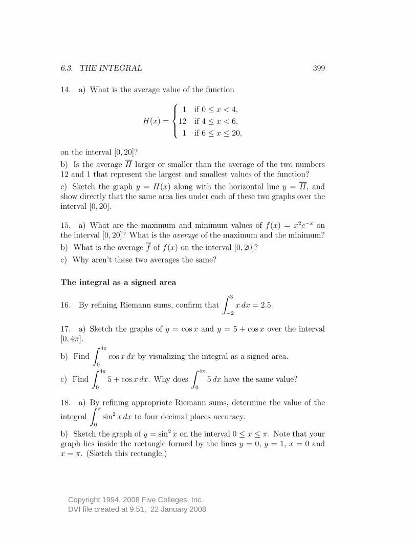
DVI file created at 9:51, 22 January 2008Copyright 1994, 2008 Five Colleges, Inc.
6.3. THE INTEGRAL 399
14. a) What is the average value of the function
H(x) =
1 if 0 ≤ x < 4,
12 if 4 ≤ x < 6,
1 if 6 ≤ x ≤ 20,
on the interval [0, 20]?
b) Is the average H larger or smaller than the average of the two numbers12 and 1 that represent the largest and smallest values of the function?
c) Sketch the graph y = H(x) along with the horizontal line y = H, andshow directly that the same area lies under each of these two graphs over theinterval [0, 20].
15. a) What are the maximum and minimum values of f(x) = x2e−x onthe interval [0, 20]? What is the average of the maximum and the minimum?
b) What is the average f of f(x) on the interval [0, 20]?
c) Why aren’t these two averages the same?
The integral as a signed area
16. By refining Riemann sums, confirm that
∫3
−2
x dx = 2.5.
17. a) Sketch the graphs of y = cos x and y = 5 + cosx over the interval[0, 4π].
b) Find
∫4π
0
cos x dx by visualizing the integral as a signed area.
c) Find
∫4π
0
5 + cos x dx. Why does
∫4π
0
5 dx have the same value?
18. a) By refining appropriate Riemann sums, determine the value of the
integral
∫ π
0
sin2 x dx to four decimal places accuracy.
b) Sketch the graph of y = sin2 x on the interval 0 ≤ x ≤ π. Note that yourgraph lies inside the rectangle formed by the lines y = 0, y = 1, x = 0 andx = π. (Sketch this rectangle.)

DVI file created at 9:51, 22 January 2008Copyright 1994, 2008 Five Colleges, Inc.
400 CHAPTER 6. THE INTEGRAL
c) Explain why the area under the graph of y = sin2 x is exactly half ofthe area of the rectangle you sketched in part (b). What is the area of thatrectangle?
d) Using your observations in part (c), explain why
∫ π
0
sin2 x dx is exactly
π/2.
19. a) On what interval a < x < b does the graph of the function y = 4−x2
lie above the x-axis?
b) Sketch the graph of y = 4− x2 on the interval a ≤ x ≤ b you determinedin part (a).
c) What is the area of the region that lies above the x-axis and below thegraph of y = 4 − x2?
20. a) What is the signed area (see page 384 in the text) between the graphof y = x3 − x and the x-axis on the interval −1 ≤ x ≤ 2?
b) Sketch the graph of y = x3 − x on the interval −1 ≤ x ≤ 2. On thebasis of your sketch, support or refute the following claim: the signed areabetween the graph of y = x3−x and the x-axis on the interval −1 ≤ x ≤ 2 isexactly the same as the area between the graph of y = x3 − x and the x-axison the interval +1 ≤ x ≤ 2.

DVI file created at 9:51, 22 January 2008Copyright 1994, 2008 Five Colleges, Inc.
6.4. THE FUNDAMENTAL THEOREM OF CALCULUS 401
6.4 The Fundamental Theorem of Calculus
Two Views of Power and Energy
In section 1 we considered how much energy a town consumed over 24hours when it was using p(t) megawatts of power at time t. Suppose E(T )megawatt-hours of energy were consumed during the first T hours. Then the Energy is the
integral of power. . .integral, introduced in section 3, gave us the language to describe how Edepends on p:
E(T ) =
∫ T
0
p(t) dt.
Because E is the integral of p, we can visualize E(T ) as the area under thepower graph y = p(t) as the time t sweeps from 0 hours to T hours:
0 6 12 18 24 hours
time
30
60
90
power
meg
awat
ts
power = p (t)area = E(T )
height = p (T )
T
As T increases, so does E(T ). The exact relation between E and T is shownin the graph below. The height of the graph of E at any point T is equal tothe area under the graph of p from 0 out to the point T .
0 6 12 18 24 hours
time
360
720
1080
1440
energy
meg
awat
t-ho
urs
height = E(T )
T
slope = p (T )
energy = E(t)

DVI file created at 9:51, 22 January 2008Copyright 1994, 2008 Five Colleges, Inc.
402 CHAPTER 6. THE INTEGRAL
The microscope window on the graph of E reminds us that the slope ofthe graph at any point T is just p(T ):
. . . and power is thederivative of energy p(T ) = E ′(T ).
We discovered this fact in section 1, where we stated it in the following form:power is the rate at which energy is consumed.
Pause now to study the graphs of power and energy. You should convinceyourself that the height of the E graph at any time equals the area under thep graph up to that time. For example, when T = 0 no area has accumulated,so E(0) = 0. Furthermore, up to T = 6 hours, power demand was almostconstant at about 30 megawatts. Therefore, E(6) should be about
30 megawatts × 6 hours = 180 megawatt-hours.
It is. You should also convince yourself that the slope of the E graph at anypoint equals the height of the p graph at that point. Thus, for example, thegraph of E will be steepest where the graph of p is tallest.
Notice that when we write the energy accumulation function E(T ) as anintegral,
E(T ) =
∫ T
0
p(t) dt,
we have introduced a new ingredient. The time variable T appears as oneA new ingredient:variable limitsof integration
of the “limits of integration.” By definition, the integral is a single number.However, that number depends on the interval of integration [0, T ]. As soonas we treat T as a variable, the integral itself becomes a variable, too. Herethe value of the integral varies with T .
We now have two ways of viewing the relation between power and energy.According to the first view, the energy accumulation function E is the integralof power demand:
E(T ) =
∫ T
0
p(t) dt.
According to the second view, the energy accumulation function is the solu-This integral isa solution to adifferential equation
tion y = E(t) to an initial value problem defined by power demand:
y′ = p(t); y(0) = 0.
If we take the first view, then we find E by refining Riemann sums—becausethat is the way to determine the value of an integral. If we take the second

DVI file created at 9:51, 22 January 2008Copyright 1994, 2008 Five Colleges, Inc.
6.4. THE FUNDAMENTAL THEOREM OF CALCULUS 403
view, then we can find E by using any of the methods for solving initialvalue problems that we studied in chapter 4. Thus, the energy integral is asolution to a certain differential equation.
This is unexpected. Differential equations involve derivatives. At firstglance, they have nothing to do with integrals. Nevertheless, the relationbetween power and energy shows us that there is a deep connection betweenderivatives and integrals. As we shall see, the connection holds for the integral The fundamental
theorem of calculusof any function. The connection is so important—because it links togetherthe two basic processes of calculus—that it has been called the fundamentaltheorem of calculus.
The fundamental theorem gives us a powerful new tool to calculate inte-grals. Our aim in this section is to see why the theorem is true, and to beginto explore its use as a tool. In Calculus II we will consider many specificintegration techniques that are based on the fundamental theorem.
Integrals and Differential Equations
We begin with a statement of the fundamental theorem for a typical functionf(x).
The Fundamental Theorem of Calculus
The solution y = A(x) to the initial value problem
y′ = f(x) y(a) = 0
is the accumulation function A(X) =
∫ X
a
f(x) dx.
We have always been able to find the value of the integral
∫ b
a
f(x) dx
by refining Riemann sums. The fundamental theorem gives us a new way. Itsays: First, find the solution y = A(x) to the initial value problem y′ = f(x),y(a) = 0 using any suitable method for solving the differential equation.Then, once we have A(x), we get the value of the integral by evaluating Aat x = b.

DVI file created at 9:51, 22 January 2008Copyright 1994, 2008 Five Colleges, Inc.
404 CHAPTER 6. THE INTEGRAL
To see how all this works, let’s find the value of the integralA test case
∫4
0
cos(x2) dx
two ways: by refining Riemann sums and by solving the initial value problem
y′ = cos(x2); y(0) = 0
using Euler’s method.To estimate the value of the integral, we use the program RIEMANNRIEMANN versus. . .
from page 362. It produces the sequence of left endpoint sums shown in thetable below on the left. Since the first three digits have stabilized, the valueof the integral is .594 . . . . The integral was deliberately chosen to lead tothe initial value problem we first considered on page 267. We solved thatproblem by Euler’s method, using the program TABLE, and produced the. . . TABLE
table of estimates for the value of y(4) that appear in the table on the right.We see y(4) = .594 . . . .
Program: RIEMANNLeft endpoint Riemann sums
DEF fnf (x) = COS(x ^ 2)
a = 0
b = 4
numberofsteps = 2 ^ 3
deltax = (b - a) / numberofsteps
x = a
accumulation = 0
FOR k = 1 TO numberofsteps
deltaS = fnf(x) * deltax
accumulation = accumulation + deltaS
x = x + deltax
NEXT k
PRINT accumulation
number estimated valueof steps of the integral
23
26
29
212
215
218
1.13304.65639.60212.59542.59458.59448
Program: TABLEEuler’s method
DEF fnf (t) = COS(t ^ 2)
tinitial = 0
tfinal = 4
numberofsteps = 2 ^ 3
deltat = (tfinal - tinitial) / numberofsteps
t = tinitial
accumulation = 0
FOR k = 1 TO numberofsteps
deltay = fnf(t) * deltat
accumulation = accumulation + deltay
t = t + deltat
NEXT k
PRINT accumulation
number estimated valueof steps of y(4)
23
26
29
212
215
218
1.13304.65639.60212.59542.59458.59448

DVI file created at 9:51, 22 January 2008Copyright 1994, 2008 Five Colleges, Inc.
6.4. THE FUNDAMENTAL THEOREM OF CALCULUS 405
RIEMANN estimates the value of an integral by calculating Riemannsums. TABLE solves a differential equation by constructing estimates usingEuler’s method. These appear to be quite different tasks, but they lead toexactly the same results! But this is no accident. Compare the programs.(In both, the PRINT statement has been put outside the loop. This speeds The two programs
are the sameup the calculations but still gives us the final outcome.) Once you makenecessary modifications (e.g., change x to t, a to tinitial, et cetera), youcan see the two programs are the same.
The very fact that these two programs do the same thing gives us oneproof of the fundamental theorem of calculus.
Graphing accumulation functions
Let’s take a closer look at the solution y = A(x) to the initial value problem
y′ = cos(x2); y(0) = 0.
We can write it as the accumulation function
A(X) =
∫ X
0
cos(x2) dx.
By switching to the graphing version of TABLE (this is the program PLOT—see page 269), we can graph A. Here is the result.
x
y
y = cos(x2 )1
−1
X
y
y = A(X ) = ⌡0
⌠ Xcos(x2 ) dx
1
1 2 3 4

DVI file created at 9:51, 22 January 2008Copyright 1994, 2008 Five Colleges, Inc.
406 CHAPTER 6. THE INTEGRAL
The relation between y = cos(x2) and y = A(x) is the same as the relationbetween power and energy.
• The height of the graph y = A(x) at any point x = X is equal tothe signed area between the graph y = cos(x2) and the x-axis over theinterval 0 ≤ x ≤ X.
• On the intervals where cos(x2) is positive, A(x) is increasing. On theintervals where cos(x2) is negative, A(x) is decreasing.
• When cos(x2) = 0, A(x) has a maximum or a minimum.
• The slope of the graph of y = A(x) at any point x = X is equal to theheight of the graph y = cos(x2) at that point.
In summary, the lower curve is the integral of the upper one, and the uppercurve is the derivative of the lower one.
x
y
X
y = ln x1
1 2 3
area = A(X ) = ⌡1
⌠ Xln x dx
x
y
X
y = A(x)
height = A(X )
1
1 2 3
To get a better idea of the simplicityand power of this approach to integrals,let’s look at another example:
A(X) =
∫ X
1
ln x dx.
The function A is the solution to the initialvalue problem
y′ = ln x, y(1) = 0;
we find it, as usual, by Euler’s method.The graphs y = lnx and y = A(x) areshown at the left. Notice once again thatthe height of the graph of A(x) at any pointx = X equals the area under the graph ofy = ln x from x = 1 to x = X. Also, thegraph of A becomes steeper as the heightof ln x increases. In particular, the graphof A is horizontal (at x = 1) when ln x = 0.
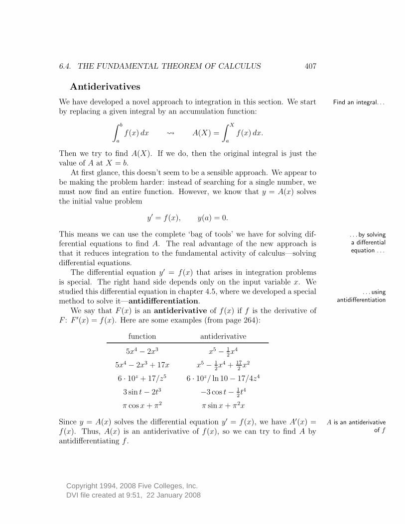
DVI file created at 9:51, 22 January 2008Copyright 1994, 2008 Five Colleges, Inc.
6.4. THE FUNDAMENTAL THEOREM OF CALCULUS 407
Antiderivatives
We have developed a novel approach to integration in this section. We start Find an integral. . .
by replacing a given integral by an accumulation function:
∫ b
a
f(x) dx A(X) =
∫ X
a
f(x) dx.
Then we try to find A(X). If we do, then the original integral is just thevalue of A at X = b.
At first glance, this doesn’t seem to be a sensible approach. We appear tobe making the problem harder: instead of searching for a single number, wemust now find an entire function. However, we know that y = A(x) solvesthe initial value problem
y′ = f(x), y(a) = 0.
This means we can use the complete ‘bag of tools’ we have for solving dif- . . . by solvinga differentialequation . . .
ferential equations to find A. The real advantage of the new approach isthat it reduces integration to the fundamental activity of calculus—solvingdifferential equations.
The differential equation y′ = f(x) that arises in integration problemsis special. The right hand side depends only on the input variable x. Westudied this differential equation in chapter 4.5, where we developed a special . . . using
antidifferentiationmethod to solve it—antidifferentiation.We say that F (x) is an antiderivative of f(x) if f is the derivative of
F : F ′(x) = f(x). Here are some examples (from page 264):
function antiderivative
5x4 − 2x3 x5 − 1
2x4
5x4 − 2x3 + 17x x5 − 1
2x4 + 17
2x2
6 · 10z + 17/z5 6 · 10z/ ln 10 − 17/4z4
3 sin t − 2t3 −3 cos t − 1
2t4
π cos x + π2 π sin x + π2x
Since y = A(x) solves the differential equation y′ = f(x), we have A′(x) = A is an antiderivativeof ff(x). Thus, A(x) is an antiderivative of f(x), so we can try to find A by
antidifferentiating f .

DVI file created at 9:51, 22 January 2008Copyright 1994, 2008 Five Colleges, Inc.
408 CHAPTER 6. THE INTEGRAL
Here is an example. Suppose we want to find
A(X) =
∫ X
2
5x4 − 2x3 dx.
Notice that f(x) = 5x4−2x3 is the first function in the previous table. SinceA must be an antiderivative of f , let’s try the antiderivative for f that wefind in the table:
F (x) = x5 − 1
2x4.
The problem is that F must also satisfy the initial condition F (2) = 0.Check the conditionA(2) = 0 However,
F (2) = 25 − 1
2· 24 = 32 − 1
2· 16 = 24 6= 0,
so the initial condition does not hold for this particular choice of antideriva-tive. But this problem is easy to fix. Let
A(x) = F (x) − 24.
Since A(x) differs from F (x) only by a constant, it has the same derivative—namely, 5x4 − 2x3. So A(x) is still an antiderivative of 5x4 − 2x3. But it alsosatisfies the initial condition:
A(2) = F (2) − 24 = 24 − 24 = 0.
Therefore A(x) solves the problem; it has the right derivative and the rightvalue at x = 2. Thus we have a formula for the accumulation function
∫ X
2
5x4 − 2x3 dx = X5 − 1
2X4 − 24.
The key step in finding the correct accumulation function A was to rec-ognize that a given function f has infinitely many antiderivatives: if F is anantiderivative, then so is F + C, for any constant C. The general procedurefor finding an accumulation function involves these two steps:
To find A(X) =
∫ X
a
f(x) dx:
1. first find an antiderivative F (x) of f(x),
2. then set A(x) = F (x) − F (a).

DVI file created at 9:51, 22 January 2008Copyright 1994, 2008 Five Colleges, Inc.
6.4. THE FUNDAMENTAL THEOREM OF CALCULUS 409
Comment: Recall that some functions f simply cannot be integrated—the A caution
Riemann sums they define may not converge. Although we have not stated itexplicitly, you should keep in mind that the procedure just described appliesonly to functions that can be integrated.
Example. To illustrate the procedure, let’s find the accumulation function
A(X) =
∫ X
0
sin x dx.
The first step is to find an antiderivative for f(x) = sin x. A natural choiceis F (x) = − cos x. To carry out the second step, note that a = 0. SinceF (0) = − cos 0 = −1, we set
A(x) = F (x) − F (0) = − cos x − (−1) = 1 − cos x.
The graphs y = sin x and y = 1 − cos x are shown below.
x
y
X
signed area = 1 − cos X
−1
1
π 2π
y = sin x
x
y
X
2
1
π 2π
y = 1 − cos x
1 − cos X
Now that we have a formula for A(x) we can find the exact value of integrals Evaluatingspecific integralsinvolving sin x. For instance,
∫ π
0
sin x dx = A(π) = 1 − cos π = 1 − (−1) = 2.
Also,∫ π/2
0
sin x dx = A(π/2) = 1 − cos π/2 = 1 − (0) = 1,

DVI file created at 9:51, 22 January 2008Copyright 1994, 2008 Five Colleges, Inc.
410 CHAPTER 6. THE INTEGRAL
and ∫2π
0
sin x dx = A(2π) = 1 − cos 2π = 1 − (1) = 0.
These values are exact, and we got them without calculating Riemannsums. However, we have already found the value of the third integral. Onpage 383 we argued from the shape of the graph y = sin x that the signedarea between x = 0 and x = 2π must be 0. That argument is no help infinding the area to x = π or to x = π/2, though. Before the fundamentaltheorem showed us we could evaluate integrals by finding antiderivatives,we could only make estimates using Riemann sums. Here, for example, aremidpoint Riemann sums for
∫ π/2
0
sin x dx :
subintervals Riemann sum
10100
100010000
1.001 028 8681.000 010 3251.000 000 1471.000 000 045
According to the table, the value of the integral is 1.000000. . . , to six deci-mal places accuracy. That is valuable information, and is often as accurateThe fundamental
theorem makesabsolute precisionpossible
as we need. However, the fundamental theorem tells us that the value ofthe integral is 1 exactly ! With the new approach, we can achieve absoluteprecision.
Precision is the result of having a formula for the antiderivative. Noticehow we used that formula to express the value of the integral. Starting withan arbitrary antiderivative F (x) of f(x), we get
A(X) =
∫ X
a
f(x) dx = F (X) − F (a).
If we set X = b we find∫ b
a
f(x) dx = F (b) − F (a).
In other words,
If F (x) is any antiderivative of f(x),
then
∫ b
a
f(x) dx = F (b) − F (a).

DVI file created at 9:51, 22 January 2008Copyright 1994, 2008 Five Colleges, Inc.
6.4. THE FUNDAMENTAL THEOREM OF CALCULUS 411
Example. Evaluate
∫ln 2
0
e−u du.
For the antiderivative, we can choose F (u) = −e−u. Then
∫ln 2
0
e−u du = F (ln 2) − F (0)
= −e− ln 2 − (−e0) = −(1/2) − (−1) = 1/2
Example. Evaluate
∫3
2
ln t dt.
For the antiderivative, we can choose F (t) = t ln t − t. Using the productrule, we can show that this is indeed an antiderivative:
F ′(t) = t · 1
t+ 1 · ln t − 1 = 1 + ln t − 1 = ln t
Thus,
∫3
2
ln t dt = F (3) − F (2)
= 3 · ln 3 − 3 − (2 · ln 2 − 2)
= ln 33 − ln 22 − 1 = ln 27 − ln 4 − 1 = ln(27/4) − 1
While formulas make it possible to get exact values, they do present uswith problems of their own. For instance, we need to know that t ln t−t is anantiderivative of ln t. This is not obvious. In fact, there is no guarantee thatthe antiderivative of a function given by a formula will have a formula! Theantiderivatives of cos(x2) and sin(x)/x do not have formulas, for instance.Many techniques have been devised to find the formula for an antiderivative.In chapter 11 of Calculus II we will survey some of those that are mostfrequently used.
Parameters
In chapter 4.2 we considered differential equations that involved parameters(see pages 214–218). It also happens that integrals can involve parameters. When integrals depend
on parameters . . .However, parameters complicate numerical work. If we calculate the value ofan integral numerically, by making estimates with Riemann sums, we mustfirst fix the value of any parameters that appear. This makes it difficult to

DVI file created at 9:51, 22 January 2008Copyright 1994, 2008 Five Colleges, Inc.
412 CHAPTER 6. THE INTEGRAL
see how the value of the integral depends on the parameters. We would haveto give new values to the parameters and then recalculate the Riemann sums.
The outcome is much simpler and more transparent if we are able to use. . . the fundamentaltheorem can help makethe relation clearer
the fundamental theorem to get a formula for the integral. The parametersjust appear in the formula, so it is immediately clear how the integral dependson the parameters.
Here is an example that we shall explore further later. We want to seehow the integrals
∫ b
a
sin(αx) dx and
∫ b
a
cos(αx) dx
depend on the parameter α 6= 0, and also on the parameters a and b. Tobegin, you should check that F (x) = − cos(αx)/α is an antiderivative ofsin(αx). Therefore,
∫ b
a
sin(αx) dx =− cos(αb)
α− − cos(αa)
α=
cos(αa) − cos(αb)
α.
In a similar way, you should be able to show that∫ b
a
cos(αx) dx =sin(αb) − sin(αa)
α.
Suppose the interval [a, b] is exactly one-half of a full period: [0, π/α]. Then∫ π/α
0
sin(αx) dx =cos(α · 0) − cos(απ/α)
α
=cos 0 − cos π
α=
1 − (−1)
α=
2
α.
Exercises
Constructing accumulation functions
1. a) Obtain a formula for the accumulation function
A(X) =
∫ X
2
5 dx
and sketch its graph on the interval 2 ≤ X ≤ 6.
b) Is A′(X) = 5?

DVI file created at 9:51, 22 January 2008Copyright 1994, 2008 Five Colleges, Inc.
6.4. THE FUNDAMENTAL THEOREM OF CALCULUS 413
2. Let f(x) = 2 + x on the interval 0 ≤ x ≤ 5.
a) Sketch the graph of y = f(x).
b) Obtain a formula for the accumulation function
A(X) =
∫ X
0
f(x) dx
and sketch its graph on the interval 0 ≤ X ≤ 5.
c) Verify that A′(X) = f(X) for every X in 0 ≤ X ≤ 5.
d) By comparing the graphs of f and A, verify that, at any point X, theslope of the graph of A is the same as the height of the graph of f .
3. a) Consider the accumulation function
A(X) =
∫ X
0
x3 dx .
Using the fact that A′(X) = X3, obtain a formula that expresses A in termsof X.
b) Modify A so that accumulation begins at the value x = 1 instead of x = 0as in part (a). Thus
A(X) =
∫ X
1
x3 dx .
It is still true that A′(X) = X3, but now A(1) = 0. Obtain a formula thatexpresses this modified A in terms of X. How do the formulas For A in parts(a) and (b) differ?
Using the fundamental theorem
4. Find A′(X) when
a) A(X) =
∫ X
0
cos(x) dx
b) A(X) =
∫ X
0
sin(x) dx
c) A(X) =
∫ X
0
cos(x2) dx
d) A(X) =
∫ X
0
cos(t2) dt
e) A(X) =
∫ X
0
sin(x2) dx
f) A(X) =
∫ X
0
sin2 x dx
g) A(X) =
∫ X
1
ln t dt
h) A(X) =
∫ X
0
x2 − 4x3 dx

DVI file created at 9:51, 22 January 2008Copyright 1994, 2008 Five Colleges, Inc.
414 CHAPTER 6. THE INTEGRAL
5. Find all critical points of the function
A(X) =
∫ X
0
cos(x2) dx
on the interval 0 ≤ X ≤ 4. Indicate which critical points are local maximaand which are local minima. (Critical points and local maxima and minimaare discussed on pages 303–309.)
[Answer: There are five critical points in the interval [0, 4]. The first is alocal maximum at
√
π/2.]
6. Find all critical points of the function
A(X) =
∫ X
0
sin(x2) dx
on the interval 0 ≤ X ≤ 4. Indicate which critical points are local maximaand which are local minima.
7. Find all critical points of the function
A(X) =
∫ X
0
x2 − 4x3 dx.
Indicate which critical points are local maxima and which are local minima.
8. Express the solution to each of the following initial value problems as anaccumulation function (that is, as an integral with a variable upper limit ofintegration).
a) y′ = cos(x2), y(√
π) = 0
b) y′ = sin(x2), y(0) = 0
c) y′ = sin(x2), y(0) = 5
d) y′ = e−x2
, y(0) = 0
9. Sketch the graphs of the following accumulation functions over the indi-cated intervals.
a)
∫ X
0
sin(x2) dx, 0 ≤ X ≤ 4
b)
∫ X
0
sin(x)
xdx, 0 ≤ X ≤ 4

DVI file created at 9:51, 22 January 2008Copyright 1994, 2008 Five Colleges, Inc.
6.4. THE FUNDAMENTAL THEOREM OF CALCULUS 415
Formulas for integrals
10. Determine the exact value of each of the following integrals.
a)
∫7
3
2 − 3x + 5x2 dx
b)
∫5π
0
sin x dx
c)
∫5π
0
sin(2x) dx
d)
∫1
0
et dt
e)
∫6
1
dx/x
f)
∫4
0
7u − 12u5du
g)
∫1
0
2t dt
h)
∫1
−1
s2 ds
11. Express the values of the following integrals in terms of the parametersthey contain.
a)
∫7
3
kx dx
b)
∫ π
0
sin(αx) dx
c)
∫4
1
px2 − x3 dx
d)
∫1
0
ect dt
e)
∫ln 3
ln 2
ect dt
f)
∫ b
1
5 − x dx
g)
∫1
0
at dt
h)
∫2
1
uc du
12. Find a formula for the solution of each of the following initial valueproblems.
a) y′ = x2 − 4x3, y(0) = 0
b) y′ = x2 − 4x3, y(3) = 0
c) y′ = x2 − 4x3, y(3) = 10
d) y′ = cos(3x), y(π) = 0
13. Find the average value of each of the following functions over the indi-cated interval.
a) x2 − x3 over [0, 1]
b) ln x over [1, e]
c) sin x over [0, π]

DVI file created at 9:51, 22 January 2008Copyright 1994, 2008 Five Colleges, Inc.
416 CHAPTER 6. THE INTEGRAL
14. a) What is the average value of the function px − x2 on the interval[0, 1]? The average depends on the parameter p.
b) For which value of p will that average be zero?
6.5 Chapter Summary
The Main Ideas
• A Riemann sum for the function f(x) on the interval [a, b] is a sumof the form
f(x1) · ∆x1 + f(x2) · ∆x2 + · · · + f(xn) · ∆xn,
where the interval [a, b] has been subdivided into n subintervals whoselengths are ∆x1, ∆x2, . . . , ∆xn, and each xk is a sampling point in thek-th subinterval (for each k from 1 to n).
• Riemann sums can be used to approximate a variety of quantities ex-pressed as products where one factor varies with the other.
• Riemann sums give more accurate approximations as the lengths∆x1, ∆x2, . . . , ∆xn are made small.
• If the Riemann sums for a function f(x) on an interval [a, b] converge,the limit is called the integral of f(x) on [a, b], and it is denoted
∫ b
a
f(x) dx.
• The units of∫ b
af(x) dx equal the product of the units of f(x) and the
units of x.
• The Fundamental Theorem of Calculus.The solution y = A(x) of the initial value problem
y′ = f(x) y(a) = 0
is the accumulation function
A(X) =
∫ X
a
f(x) dx.

DVI file created at 9:51, 22 January 2008Copyright 1994, 2008 Five Colleges, Inc.
6.5. CHAPTER SUMMARY 417
• If F (x) is an antiderivative of f(x), then
∫ b
a
f(x) dx = F (b) − F (a).
• The integral∫ b
af(x) dx equals the signed area between the graph of
f(x) and the x-axis.
• If f(x) is monotonic on [a, b] and if∫ b
af(x) dx is approximated by a
Riemann sum with subintervals of width ∆x, then the error in theapproximation is at most ∆x · |f(b) − f(a)|.
Self-Testing
• You should be able to write down (by hand) a Riemann sum to approx-imate a quantity expressed as a product (e.g., human effort, electricalenergy, work, distance travelled, area).
• You should be able to write down an integral giving the exact value ofa quantity approximated by a Riemann sum.
• You should be able to use sigma notation to abbreviate a sum, andyou should be able to read sigma notation to calculate a sum.
• You should be able to use a computer program to compute the valueof a Riemann sum.
• You should be able to find an error bound when approximating anintegral by a Riemann sum.
• You should know and be able to use the integration rules.
• You should be able to use the fundamental theorem of calculus to findthe value of an integral.
• You should be able to use an antiderivative to find the value of anintegral.

DVI file created at 9:51, 22 January 2008Copyright 1994, 2008 Five Colleges, Inc.
418 CHAPTER 6. THE INTEGRAL