Chapter 6 Scatterplots, Association and...
63
Chapter 6 Scatterplots, Association and Correlation
Transcript of Chapter 6 Scatterplots, Association and...

Chapter 6 Scatterplots, Association andCorrelation

Looking for Correlation
ExampleDoes the number of hours you watch TV per week impact youraverage grade in a class?
Hours 12 10 5 3 15 16 8Grade 70 85 82 88 65 75 68
To see if there is a relationship, we will create a scatterplot andanalyze it.
DefinitionA scatterplot is a geographical representation between twoquantitative variables. They may be from the same individual (i.e.education v. income, height v. weight) or from paired individuals (i.e.age of partners in a relationship).
Scatterplots
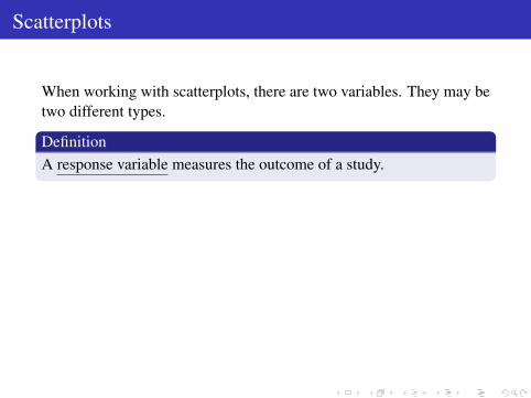
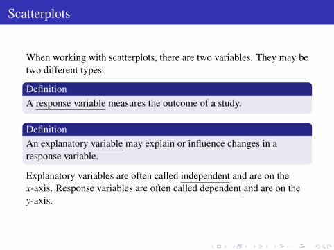
When working with scatterplots, there are two variables. They may betwo different types.
DefinitionA response variable measures the outcome of a study.
DefinitionAn explanatory variable may explain or influence changes in aresponse variable.
Explanatory variables are often called independent and are on thex-axis. Response variables are often called dependent and are on they-axis.

Scatterplots
When working with scatterplots, there are two variables. They may betwo different types.
DefinitionA response variable measures the outcome of a study.
DefinitionAn explanatory variable may explain or influence changes in aresponse variable.
Explanatory variables are often called independent and are on thex-axis. Response variables are often called dependent and are on they-axis.

Back to Our Example
In our example, which is the explanatory variable?
Watched TV hours.
The response variable is there for the average grade. So the questionwe are trying to answer is “Does watching TV influence the averagegrade in a class?”
Let’s plot the data and see what we have.
Back to Our Example
In our example, which is the explanatory variable?
Watched TV hours.
The response variable is there for the average grade. So the questionwe are trying to answer is “Does watching TV influence the averagegrade in a class?”
Let’s plot the data and see what we have.
Back to Our Example
In our example, which is the explanatory variable?
Watched TV hours.
The response variable is there for the average grade. So the questionwe are trying to answer is “Does watching TV influence the averagegrade in a class?”
Let’s plot the data and see what we have.

Back to Our Example
In our example, which is the explanatory variable?
Watched TV hours.
The response variable is there for the average grade. So the questionwe are trying to answer is “Does watching TV influence the averagegrade in a class?”
Let’s plot the data and see what we have.

The Scatterplot
Grades v. Hours of TV
Hours of TV
Gra
de
70
80
90
65
75
85
5 10 15
•
••
•
•
•
•
How Does the Relationship Look?
What do we think?
It looks like the more hours of TV that are watched, the lower theaverage grade. But how good is the relationship? We can measure thisin different ways. One is direction (+,−) and another is by rankingthe strength. These are both accomplished by looking at thecorrelation coefficient.

Facts About Correlation Coefficients:
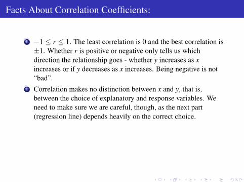
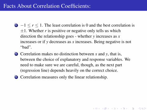
1 −1 ≤ r ≤ 1. The least correlation is 0 and the best correlation is±1. Whether r is positive or negative only tells us whichdirection the relationship goes - whether y increases as xincreases or if y decreases as x increases. Being negative is not“bad”.
2 Correlation makes no distinction between x and y, that is,between the choice of explanatory and response variables. Weneed to make sure we are careful, though, as the next part(regression line) depends heavily on the correct choice.
3 Correlation measures only the linear relationship.4 Correlation is not resistant.5 Correlation has no units.
Facts About Correlation Coefficients:
1 −1 ≤ r ≤ 1. The least correlation is 0 and the best correlation is±1. Whether r is positive or negative only tells us whichdirection the relationship goes - whether y increases as xincreases or if y decreases as x increases. Being negative is not“bad”.
2 Correlation makes no distinction between x and y, that is,between the choice of explanatory and response variables. Weneed to make sure we are careful, though, as the next part(regression line) depends heavily on the correct choice.
3 Correlation measures only the linear relationship.
4 Correlation is not resistant.5 Correlation has no units.

Facts About Correlation Coefficients:
1 −1 ≤ r ≤ 1. The least correlation is 0 and the best correlation is±1. Whether r is positive or negative only tells us whichdirection the relationship goes - whether y increases as xincreases or if y decreases as x increases. Being negative is not“bad”.
2 Correlation makes no distinction between x and y, that is,between the choice of explanatory and response variables. Weneed to make sure we are careful, though, as the next part(regression line) depends heavily on the correct choice.
3 Correlation measures only the linear relationship.4 Correlation is not resistant.
5 Correlation has no units.

Facts About Correlation Coefficients:
1 −1 ≤ r ≤ 1. The least correlation is 0 and the best correlation is±1. Whether r is positive or negative only tells us whichdirection the relationship goes - whether y increases as xincreases or if y decreases as x increases. Being negative is not“bad”.
2 Correlation makes no distinction between x and y, that is,between the choice of explanatory and response variables. Weneed to make sure we are careful, though, as the next part(regression line) depends heavily on the correct choice.
3 Correlation measures only the linear relationship.4 Correlation is not resistant.5 Correlation has no units.

So How Do We Find This Correlation Coefficient?
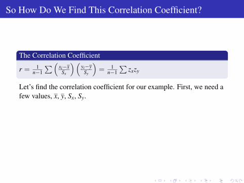
The Correlation Coefficient
r = 1n−1
∑(xi−x
Sx
)(yi−y
Sy
)= 1
n−1∑
zxzy
Let’s find the correlation coefficient for our example. First, we need afew values, x, y, Sx, Sy.
x = 9.857 y = 76.143Sx = 4.880 Sy = 8.971
So How Do We Find This Correlation Coefficient?
The Correlation Coefficient
r = 1n−1
∑(xi−x
Sx
)(yi−y
Sy
)= 1
n−1∑
zxzy
Let’s find the correlation coefficient for our example. First, we need afew values, x, y, Sx, Sy.
x = 9.857 y = 76.143Sx = 4.880 Sy = 8.971

So How Do We Find This Correlation Coefficient?
The Correlation Coefficient
r = 1n−1
∑(xi−x
Sx
)(yi−y
Sy
)= 1
n−1∑
zxzy
Let’s find the correlation coefficient for our example. First, we need afew values, x, y, Sx, Sy.
x = 9.857 y = 76.143Sx = 4.880 Sy = 8.971
Finding the Correlation Coefficient
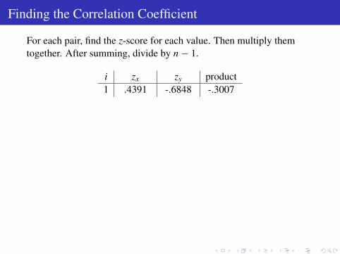
For each pair, find the z-score for each value. Then multiply themtogether. After summing, divide by n− 1.
i zx zy product1 .4391 -.6848 -.3007
2 .0293 .9873 .02893 -.9953 .6529 -.64984 -1.4050 1.3217 -1.85705 1.0539 -1.2421 -1.30906 1.2588 -.1274 -.16047 -.3805 -.9077 .3454
-3.9026
r =16(−3.9026) = −.6504
Interpretation: Moderate negative correlation

Finding the Correlation Coefficient
For each pair, find the z-score for each value. Then multiply themtogether. After summing, divide by n− 1.
i zx zy product1 .4391 -.6848 -.30072 .0293 .9873 .02893 -.9953 .6529 -.64984 -1.4050 1.3217 -1.85705 1.0539 -1.2421 -1.30906 1.2588 -.1274 -.16047 -.3805 -.9077 .3454
-3.9026
r =16(−3.9026) = −.6504
Interpretation: Moderate negative correlation

So Can We Say There Is A Relationship?
So, can we say that there is a direct relationship between the numberof hours of TV watched and the average grade? Not so fast ...
Correlation does not necessarily imply causation.
Just because it looks the part does not mean we have evidence thatthere is a relationship. We have to consider a couple of other things.One is lurking variables. These are variables that may be present butwe are not actually considering them within the data.
Can you think of any lurking variables that would impact ourexample?
Significance
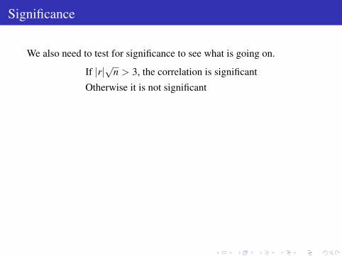
We also need to test for significance to see what is going on.
If |r|√
n > 3, the correlation is significant
Otherwise it is not significant
The smaller this value, the smaller the probability that the correlationwill be significant.
Reasons why data may not be significant:1 Genuine lack of correlation2 Not enough data
Our example is not significant because of quantity. So we cannotconsider that watching TV has a direct impact on grades.
Significance
We also need to test for significance to see what is going on.
If |r|√
n > 3, the correlation is significant
Otherwise it is not significant
The smaller this value, the smaller the probability that the correlationwill be significant.
Reasons why data may not be significant:1 Genuine lack of correlation
2 Not enough data
Our example is not significant because of quantity. So we cannotconsider that watching TV has a direct impact on grades.

Significance
We also need to test for significance to see what is going on.
If |r|√
n > 3, the correlation is significant
Otherwise it is not significant
The smaller this value, the smaller the probability that the correlationwill be significant.
Reasons why data may not be significant:1 Genuine lack of correlation2 Not enough data
Our example is not significant because of quantity. So we cannotconsider that watching TV has a direct impact on grades.

Assumptions and Conditions for Correlation
Quantitative Variables ConditionDon’t make the common error of calling an association involvinga categorical variable a correlation. Correlation is only aboutquantitative variables.
Straight Enough ConditionThe best check for the assumption that the variables are trulylinearly related is to look at the scatterplot to see whether it looksreasonably straight. That’s a judgment call, but not a difficultone.
No Outliers ConditionOutliers can distort the correlation dramatically, making a weakassociation look strong or a strong one look weak. Outliers caneven change the sign of the correlation. But it’s easy to seeoutlier in the scatterplot, so to check this condition, just look.

Another Example
ExampleThe following gives the power numbers for the starting 9 for the 2007Boston Red Sox. Is there relationship between the number of homeruns and the number of RBIs? Does the number of home runs affectthe number of RBIs? Produce a scatterplot and discuss the correlation.
Player Home Runs RBIsVaritek 17 68Youkilis 16 83Pedroia 8 50Lowell 21 120Lugo 8 73Ramirez 20 88Crisp 6 60Drew 11 64Ortiz 35 117

Red Sox Example
Which is the response variable? Which is the response variable?
Since we are asking if HR affects RBIs, HR would be the explanatoryvariable and therefore x. So RBIs is the y variable.
2007 Red Sox Power Numbers
Home Runs
RB
Is
40
80
120
20
60
100
10 20 30
••
•
•
••
• •
•

Red Sox Example
Which is the response variable? Which is the response variable?
Since we are asking if HR affects RBIs, HR would be the explanatoryvariable and therefore x. So RBIs is the y variable.
2007 Red Sox Power Numbers
Home Runs
RB
Is
40
80
120
20
60
100
10 20 30
••
•
•
••
• •
•

Before We Go On
Something to notice: we have two values with the same x-coordinate.
2007 Red Sox Power Numbers
Home Runs
RB
Is
40
80
120
20
60
100
10 20 30
••
•
•
••
• •
•

Finding the Correlation Coefficient
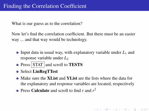
What is our guess as to the correlation?
Now let’s find the correlation coefficient. But there must be an easierway ... and that way would be technology.
Input data in usual way, with explanatory variable under L1 andresponse variable under L2
Press STAT and scroll to TESTSSelect LinRegTTestMake sure the XList and YList are the lists where the data forthe explanatory and response variables are located, respectively
Press Calculate and scroll to find r and r2

Finding the Correlation Coefficient
What is our guess as to the correlation?
Now let’s find the correlation coefficient. But there must be an easierway ... and that way would be technology.
Input data in usual way, with explanatory variable under L1 andresponse variable under L2
Press STAT and scroll to TESTS
Select LinRegTTestMake sure the XList and YList are the lists where the data forthe explanatory and response variables are located, respectively
Press Calculate and scroll to find r and r2

Finding the Correlation Coefficient
What is our guess as to the correlation?
Now let’s find the correlation coefficient. But there must be an easierway ... and that way would be technology.
Input data in usual way, with explanatory variable under L1 andresponse variable under L2
Press STAT and scroll to TESTSSelect LinRegTTest
Make sure the XList and YList are the lists where the data forthe explanatory and response variables are located, respectively
Press Calculate and scroll to find r and r2

Finding the Correlation Coefficient
What is our guess as to the correlation?
Now let’s find the correlation coefficient. But there must be an easierway ... and that way would be technology.
Input data in usual way, with explanatory variable under L1 andresponse variable under L2
Press STAT and scroll to TESTSSelect LinRegTTestMake sure the XList and YList are the lists where the data forthe explanatory and response variables are located, respectively
Press Calculate and scroll to find r and r2

Using Technology
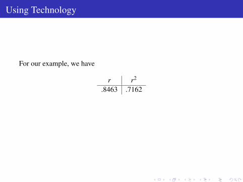
For our example, we have
r r2
.8463 .7162
So the correlation coefficient tells us that there is a strong positivecorrelation.
Using Technology
For our example, we have
r r2
.8463 .7162
So the correlation coefficient tells us that there is a strong positivecorrelation.

Using Technology
For our example, we have
r r2
.8463 .7162
So the correlation coefficient tells us that there is a strong positivecorrelation.

What Does r2 Tell Us?
r2 tells us how much better our predictions will be if we go throughthe trouble to find the regression line rather than just make ourpredictions with the means. Ours is pretty good here, indicating thatwe should find the regression line.
2007 Red Sox Power Numbers
Home Runs
RB
Is
40
80
120
20
60
100
10 20 30
••
•
•
••
• •
•

Technology and Scatterplots
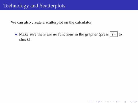
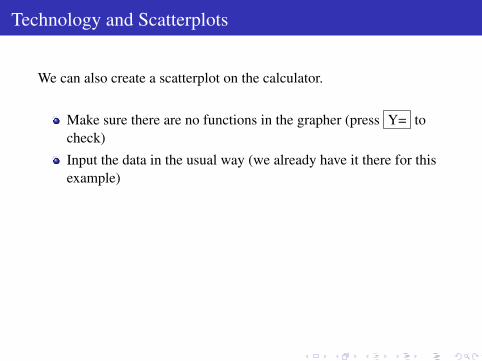
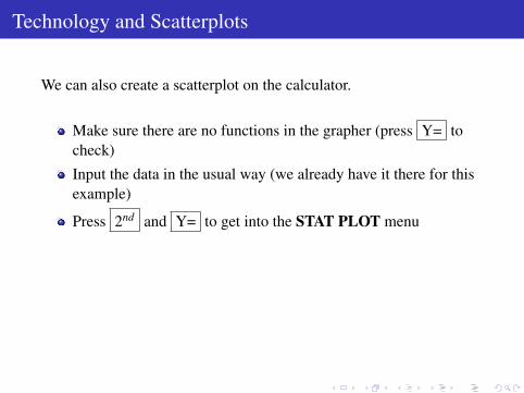
We can also create a scatterplot on the calculator.
Make sure there are no functions in the grapher (press Y= tocheck)
Input the data in the usual way (we already have it there for thisexample)
Press 2nd and Y= to get into the STAT PLOT menu
Make sure only the plot we want is turned on
Select the first graph in the first row and then make sure theXList and YList are correct
Press ZOOM 9
Technology and Scatterplots
We can also create a scatterplot on the calculator.
Make sure there are no functions in the grapher (press Y= tocheck)
Input the data in the usual way (we already have it there for thisexample)
Press 2nd and Y= to get into the STAT PLOT menu
Make sure only the plot we want is turned on
Select the first graph in the first row and then make sure theXList and YList are correct
Press ZOOM 9
One More Example
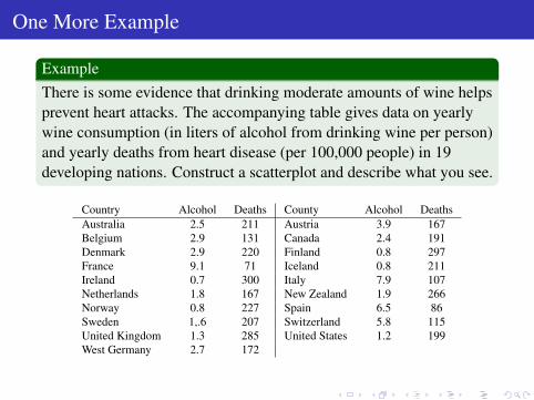
ExampleThere is some evidence that drinking moderate amounts of wine helpsprevent heart attacks. The accompanying table gives data on yearlywine consumption (in liters of alcohol from drinking wine per person)and yearly deaths from heart disease (per 100,000 people) in 19developing nations. Construct a scatterplot and describe what you see.
Country Alcohol Deaths County Alcohol DeathsAustralia 2.5 211 Austria 3.9 167Belgium 2.9 131 Canada 2.4 191Denmark 2.9 220 Finland 0.8 297France 9.1 71 Iceland 0.8 211Ireland 0.7 300 Italy 7.9 107Netherlands 1.8 167 New Zealand 1.9 266Norway 0.8 227 Spain 6.5 86Sweden 1,.6 207 Switzerland 5.8 115United Kingdom 1.3 285 United States 1.2 199West Germany 2.7 172

The Scatterplot
Heart Disease v. Alcohol from Wine
Alcohol from Wine (in liters)
Dea
ths
(per
100,
000)
100
200
300
50
150
250
2 4 6 8
••
•
••
•
•
•
•
•
•
••
•
•
•
•
••
r = −.8428, strong negative correlation
r2 = .7103, worthwhile to find linear regression line

The Scatterplot
Heart Disease v. Alcohol from Wine
Alcohol from Wine (in liters)
Dea
ths
(per
100,
000)
100
200
300
50
150
250
2 4 6 8
••
•
••
•
•
•
•
•
•
••
•
•
•
•
••
r = −.8428, strong negative correlation
r2 = .7103, worthwhile to find linear regression line

The Scatterplot
Heart Disease v. Alcohol from Wine
Alcohol from Wine (in liters)
Dea
ths
(per
100,
000)
100
200
300
50
150
250
2 4 6 8
••
•
••
•
•
•
•
•
•
••
•
•
•
•
••
r = −.8428, strong negative correlation
r2 = .7103, worthwhile to find linear regression line