Chapter 6 I Law for Control Volume - IIT Madrasamitk/AS1300/ControlVolume.pdf · Chapter 6 I Law...
12
Chapter 6 I Law for Control Volume 6.1 Introduction In Chapter 1, ‘Control Volume’ was defined as a fixed volume on which attention is focused. Apart from energy interactions in the form of heat or work with the surroundings, it can also admit in-flow (m i ) or out-flow of mass (m e ) through inlet or exit, respectively. Practical devices involving the flow of a fluid, such as a turbine, pump, compressor, nozzle, valve, boiler, condenser, etc. can be modeled as CV. The form of I Law for a Control Volume is different from that of a system, on account of the fact that there is mass exchange. Moreover, in addition to the internal energy, forms of energy storage such as the kinetic energy and potential energy could be important in many cases. Fig. 6.1 Control Volume Analysis Let us now turn our attention to the modes of work interaction. For a control volume, the work interaction W cannot include displacement work (i.e. work of expansion or compression). This is because of the fact that the volume of CV remains constant. Other forms such as electrical work, magnetic work, shaft work etc. could be included in W. Some authors call this W as ‘external work’, implying that there is also some internal work within the fluid. For instance, the incoming mass m i pushes the fluid ahead of it, like a piston. Similarly, the outgoing mass m e also pushes the fluid ahead of it. This form of work is known as the ‘flow work’ and it is given by the expression (m.p.v), where p and v are the local pressure and the local fluid specific volume. More explanation on flow work is provided subsequently. Surroundings Q W m e m i Control Volume ME1100 Thermodynamics Lecture Notes Prof. T. Sundararajan Dept. of Mechanical Engineering Indian Institute of Technology Madras
Transcript of Chapter 6 I Law for Control Volume - IIT Madrasamitk/AS1300/ControlVolume.pdf · Chapter 6 I Law...

Chapter 6 I Law for Control Volume
6.1 Introduction
In Chapter 1, ‘Control Volume’ was defined as a fixed volume on which attention is
focused. Apart from energy interactions in the form of heat or work with the
surroundings, it can also admit in-flow (mi) or out-flow of mass (me) through inlet or
exit, respectively. Practical devices involving the flow of a fluid, such as a turbine, pump,
compressor, nozzle, valve, boiler, condenser, etc. can be modeled as CV. The form of I
Law for a Control Volume is different from that of a system, on account of the fact that
there is mass exchange. Moreover, in addition to the internal energy, forms of energy
storage such as the kinetic energy and potential energy could be important in many
cases.
Fig. 6.1 Control Volume Analysis
Let us now turn our attention to the modes of work interaction. For a control volume,
the work interaction W cannot include displacement work (i.e. work of expansion or
compression). This is because of the fact that the volume of CV remains constant. Other
forms such as electrical work, magnetic work, shaft work etc. could be included in W.
Some authors call this W as ‘external work’, implying that there is also some internal
work within the fluid. For instance, the incoming mass mi pushes the fluid ahead of it,
like a piston. Similarly, the outgoing mass me also pushes the fluid ahead of it. This form
of work is known as the ‘flow work’ and it is given by the expression (m.p.v), where p
and v are the local pressure and the local fluid specific volume. More explanation on flow
work is provided subsequently.
Control Volume
Surroundings
Q
W
me
mi Control
Volume
ME1100 Thermodynamics Lecture Notes Prof. T. Sundararajan
Dept. of Mechanical Engineering Indian Institute of Technology Madras

6.2 Derivation of I Law for a CV
Let us now derive the energy balance (I law) principle for a control volume. For
the sake of simplicity, let us consider a single inlet and single outlet situation, although
the energy balance can be generalized later on, to the case of multiple inlets and
outlets. For obtaining the I law for CV, we shall use the familiar I law for a system over
a small time interval t. In other words, we shall consider two time instants ‘t’ and
‘t+t’, when a system of given mass occupies the control volume as shown in Fig. 6.2.
(a)
(b)
Fig. 6.2 Energy balance for fixed mass over time interval t
The same mass (Fig. 6.2 a) which consists of dmi + MCV(t) at time ‘t’, occupies the
configuration dme + MCV(t+t) at time ‘t+t’ (Fig. 6.2 b). Here, dmi and dme are the
masses that enter into or exit from the control volume over the time interval t. Also,
MCV(t) and MCV(t+t) are the masses that occupy the control volume at time ‘t’ and time
‘t+t’ respectively.
Now, the total energy of the system at time ‘t’ is equal to :
At time t
Q W
dmi
MCV(t)
ze zi
pi
Q W
dme
MCV(t+t)
At time t+t
pe
ME1100 Thermodynamics Lecture Notes Prof. T. Sundararajan
Dept. of Mechanical Engineering Indian Institute of Technology Madras

)
2()(
2
ii
iiCV zgV
udmtE
where ECV(t) is the total energy (internal + kinetic + potential energy) stored in the
control volume at time ‘t’. Also, the second term represents the total energy (internal +
kinetic + potential energy) brought by the incoming mass dmi. Here, Vi is the inlet flow
velocity and zi is the elevation of the inlet. Similarly, the total energy of the system at
time ‘t+t’ can be written as
)2
()(2
ee
eeCV zgV
udmttE .
The first and second terms of the above expression represent the energy stored in the
CV at time ‘t+t’ and the total energy carried away by the out-going mass dme.
Now, applying I law for the system (fixed mass under consideration), we can write:
Heat added – Work done = Change in total energy.
The work interaction consists of the work W done across the CV boundary and also the
flow work at the inlet and the flow work at the exit. The flow work at the inlet is
negative, because fluid which is flowing towards the CV is doing work on the system
under consideration. This work can be evaluated as:
Flow work at the inlet = - pi . dVi .
Here dVi is the volume of fluid flowing against the resisting pressure of pi at the inlet
(Fig. 6.2 a), within the time interval of ‘t’ and ‘t+t’ . The volume dVi can be calculated
as dmi.vi , where vi is the specific volume of fluid in the inlet region. Thus, the flow work
at inlet can be expressed as – dmi (pivi). Similarly, the flow work at the outlet is given as
+ dme (peve). Now, application of I law for the system under consideration gives:
ME1100 Thermodynamics Lecture Notes Prof. T. Sundararajan
Dept. of Mechanical Engineering Indian Institute of Technology Madras

Q – {W + dme (peve) - dmi (pivi)} = { )2
()(2
ee
eeCV zgV
udmttE } -
{ )2
()(2
ii
iiCV zgV
udmtE }
After rearranging the terms, we get:
}2
{
}2
{)()(
2
2
ii
iiii
ee
eeeeCVCV
zgV
vpudm
zgV
vpudmtEttEWQ
Since specific enthalpy h = u + pv, this expression can be simplified as
}2
{}2
{
}2
{}2
{)()(
22
22
ii
iiee
eeCV
ii
iiee
eeCVCV
zgV
hdmzgV
hdmdE
zgV
hdmzgV
hdmtEttEWQ
Now, dividing the above energy balance expression by the time interval t and taking
the limit as t 0, results in the equation
}2
{}2
{22
ii
iiee
eeCV zg
Vhmzg
Vhm
dt
dEWQ
. (6.1)
The terms on the left hand side of Eq. (6.1) refer to the rate of heat addition and the
rate of work done across the control volume boundary. The first term on the right hand
side refers to the rate of total energy storage in the CV. The second term on RHS
includes the rate of total energy carried by the out flow and the rate of flow work done
at the exit. Remember that enthalpy h includes the internal energy ‘u’ and the flow work
‘pv’ per kg of flow. The last term on RHS represents the rate of total energy brought by
ME1100 Thermodynamics Lecture Notes Prof. T. Sundararajan
Dept. of Mechanical Engineering Indian Institute of Technology Madras

the inflow and the rate of flow work done at the inlet. In the case of a problem with
multiple inlets and exits, the equation (6.1) can be modified to a more general form
i
ii
ii
e
ee
eeCV zg
Vhmzg
Vhm
dt
dEWQ }
2{}
2{
22
. (6.2)
Here the summations are taken over all the exits ‘e’ and the inlets ‘i’. The applications of
I law for a CV can be brought under two major classifications, namely, those of steady
flow devices and unsteady flow devices. In the case of a thermal power plant which
carries out energy conversion from heat to work, many of the sub-components can be
modeled as Control Volumes, as discussed below. The steam generator or boiler, takes
in heat input and converts water into steam at high pressure and temperature. A steam
turbine is a device in which the high pressure steam impinges on the blades and
produces rotary motion (i.e. generates shaft work). In the condenser, steam (after
transferring part of its energy as work in the turbine) is condensed back to water. A
pump raises the pressure of the condensed water and sends it back to the steam
generator (Fig. 6.2 a). Since a power plant operates in a continuous mode, except for
some occasional shut-downs, it is meaningful to analyze the associated components as
steady flow devices.
Fig. 6.2 a Schematic of Thermal Power Plant
Condenser
Steam
Turbine
Pump
Qinput
Steam
generator
Winput
Qrejected
Wturbine
Water
Water Steam
Steam
ME1100 Thermodynamics Lecture Notes Prof. T. Sundararajan
Dept. of Mechanical Engineering Indian Institute of Technology Madras

In a typical aero-engine, atmospheric air which enters at a high relative velocity
(because of the high speed of the aircraft) is slowed down in a diffuser, which converts
the kinetic energy into pressure. The air is further compressed in a compressor and sent
to the combustor where it burns with a fuel and produces heat. The hot products of
combustion expand in a turbine producing mechanical (shaft) work. Finally, the hot
combustion products are further expanded in a nozzle, generating a high speed jet
exhaust. The high momentum jet generates forward thrust according to Newton’s III
law (Fig. 6.2 b). During the continuous operation of the engine, steady flow analysis
could be carried out for each component, using the I law for a CV.
Fig. 6.2 b Schematic of Aero-engine system
6.3 Steady Flow Devices
Let us now consider the steady flow operation of various devices. Under the steady flow
assumption, accumulation of mass or energy within the CV is taken to be zero. In other
words, at every instant, the rate of inflow of mass to the CV is equal to the rate of out-
flow from the CV. Also, the rate at which energy enters the CV (as heat, work or energy
Air
Fuel
Gas Turbine Compressor
Combustor
Diffuser Nozzle
Exhaust
ME1100 Thermodynamics Lecture Notes Prof. T. Sundararajan
Dept. of Mechanical Engineering Indian Institute of Technology Madras

of the flowing mass) is equal to the rate at which it leaves the control volume. Thus for
steady state, we can set
0dt
dECV
With this simplification, equation (6.1) for a single inlet- single outlet device can be
rewritten as:
.
)}(2
{
}2
{}2
{
22
22
devicethethroughrateflowmassmmmwhere
zzgVV
hhm
zgV
hmzgV
hmWQ
ie
ieie
ie
ii
iiee
ee
(6.3)
Now let us look at further simplifications for specific devices.
(i) Adiabatic devices:
We came across devices such as steam turbine, gas turbine, compressor, pump, nozzle,
diffuser, etc. in our discussions about the steam power plant and the aero-engine. In
ideal situations, these devices are supposed to be adiabatic. For example, an ideal
steam turbine is supposed to convert the energy contained in steam into useful
mechanical work, without any heat losses to the surroundings. Therefore, we can set
rate of heat transfer = 0 for the turbine. Furthermore, for any device dealing with gas
flow, the potential energy difference can be neglected. (The potential energy term will
be important only for devices handling liquid flows, especially when the height
differences are significant.) Thus, we can neglect the term of g.(ze – zi). In many cases,
even the kinetic energy term may be negligible. Then I law for a steam turbine simplifies
as
)()( eiie hhmWhhmW (6.4a)
The above expression implies that the power developed by the turbine is equal to the
product of steam mass flow rate and the decrease of steam enthalpy from the inlet to
ME1100 Thermodynamics Lecture Notes Prof. T. Sundararajan
Dept. of Mechanical Engineering Indian Institute of Technology Madras

the outlet. When the kinetic energy change is important, the I law for the turbine can be
written as
}2
){(22
ieie
VVhhmW
(6.4b)
Equations (6.4a) or (6.4b) are valid also for a gas turbine, which operates with the
combustion product gas as working fluid. One can assume the product gas to be an
ideal gas and calculate the properties using ideal gas relations. The steam turbine and
gas turbine are positive work producing devices. The expressions (6.4a) and (6.4b) can
be used for the analyzing the compressor also. In the example shown in Fig. 6.2b, the
compressor compresses the air (air density, pressure and temperature will increase
because of compression) by taking work input from the turbine. Just as a compressor
increases the pressure of a gas, a pump will increase the pressure of a liquid with the
help of work input. The increase in pressure will result in the increase of enthalpy from
the inlet to the outlet of the pump. Thus, Eq. (6.4a) is valid for a pump also. Normally,
the change in kinetic energy can be neglected for a pump, because of low velocities.
Also, the change in potential energy can be neglected because the height differences
between the inlet and outlet are usually small.
From the above discussion, it is clear that W> 0 for a turbine, while W < 0 for a pump
or a compressor. In adiabatic devices such as nozzle or diffuser, heat as well as work
interactions are zero. Consider an adiabatic nozzle with steady flow, as shown in Fig.
6.5a.
Fig. 6.5a Adiabatic nozzle
Since both heat transfer and work done are zero, the I law simplifies to the form:
Vi Ve
ME1100 Thermodynamics Lecture Notes Prof. T. Sundararajan
Dept. of Mechanical Engineering Indian Institute of Technology Madras
22
22
ee
ii
Vh
Vh (6.5)
Often, the inlet kinetic energy may be neglected and this leads to the simplification
)(2 eie hhV (6.6)
for the nozzle exit velocity. For steady flow, we can also apply the mass balance
principle as follows:
mAVmAVm eeeeiiii (6.7)
The above expression implies that the mass flow rates at the inlet and the outlet are
both equal to the overall flow rate of m through the nozzle. Also, the mass flow rate is
given as the product of the density, velocity and flow area at the inlet or outlet. It is
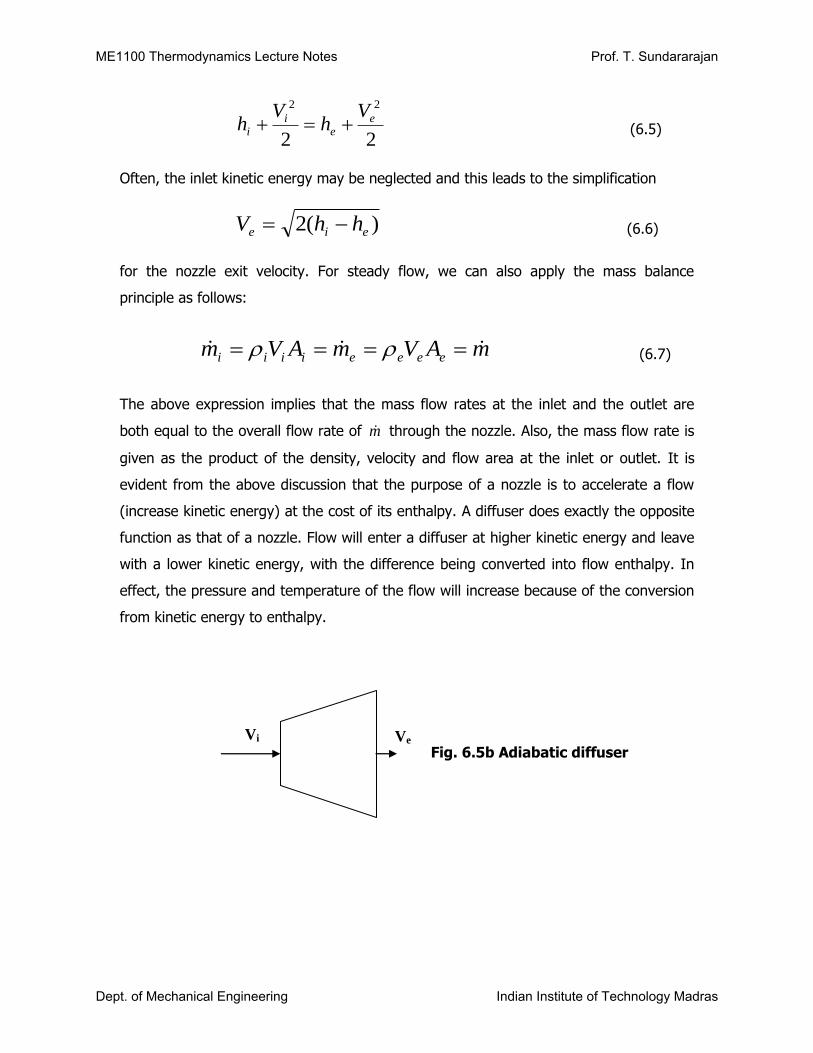
evident from the above discussion that the purpose of a nozzle is to accelerate a flow
(increase kinetic energy) at the cost of its enthalpy. A diffuser does exactly the opposite
function as that of a nozzle. Flow will enter a diffuser at higher kinetic energy and leave
with a lower kinetic energy, with the difference being converted into flow enthalpy. In
effect, the pressure and temperature of the flow will increase because of the conversion
from kinetic energy to enthalpy.
Fig. 6.5b Adiabatic diffuser
Vi Ve
ME1100 Thermodynamics Lecture Notes Prof. T. Sundararajan
Dept. of Mechanical Engineering Indian Institute of Technology Madras

Finally, we consider the device of throttle valve which is used for controlling the flow
rates in pipe lines and other fluid equipment. The heat and work interactions for a
throttle valve may be taken as zero. Moreover, the changes in kinetic energy and
potential energy are also negligible. This leads to the expression
ei hh (6.7)
Enthalpy being constant does not mean that the states of the flow before and after the
throttle valve are exactly the same. In fact, as shown in Fig. 6.6, the fluid rapidly
expands across the valve without having contributed any useful work.
Fig. 6.6 Flow through a Throttle Valve
This type of rapid flow expansion across a valve is known as a ‘throttling process’ and
since enthalpy is constant, it is also called as an ‘isenthalpic process’. So far, we have
discussed applications in which steady flow assumption can be applied to devices that
are adiabatic (heat transfer is zero). We shall now look at steady flow devices which
involve heat transfer.
(ii) Heat exchange devices:
Devices such as steam generator (boiler), condenser , evaporator in a refrigerator etc.
are examples of heat exchange devices. In a steam generator, water enters in liquid
phase and due to heat addition, it is converted into steam at high temperature. No
external work is done in the device and the changes in kinetic energy & potential energy
are usually negligible. Therefore, the I law for steam generator can be simplified to the
form
ME1100 Thermodynamics Lecture Notes Prof. T. Sundararajan
Dept. of Mechanical Engineering Indian Institute of Technology Madras

)( ie hhmQ (6.8)
The above form of I law is applicable to the condenser also. In a condenser, as seen
from Fig. 6.2a, steam at low p and T is condensed back as water, by the removal of
heat. Thus, Q > 0 for boiler while Q < 0 for condenser. Correspondingly, the enthalpy
increases across the boiler while it decreases across the condenser. In a refrigerator, the
refrigerant fluid evaporates by absorbing heat from food stuff, in the evaporator. Thus,
Eq. (6.8) can be applied for the evaporator also, with a positive value of Q.
In devices like boiler or condenser, the heat addition or heat removal is not done
directly. Usually, another fluid is used for this purpose. For example, in the case of
boiler, the combustion gases generated from the burning of coal in air are circulated
around tubes carrying water. Therefore, heat is transferred from the hot combustion gas
to the water, for producing steam. Also, in the case of the condenser, sea water may
circulated around tubes carrying steam for cooling purposes. There is no direct heat
transfer between the surroundings and the CV in such cases. Thus, we can analyze
these situations as devices with multiple inlet and exit streams, as shown in Figs. 6.7a
and 6.7b.
6.7b Condenser
6.7a Boiler
Cooling
water inlet
Cooling
water outlet
Steam Water
Steam
Water
Combustion
gas
Combustion
gas
ME1100 Thermodynamics Lecture Notes Prof. T. Sundararajan
Dept. of Mechanical Engineering Indian Institute of Technology Madras

The first law for these devices can be expressed as:
0 i
i
i
e
ee hmhm (6.9)
between the different inlet and exit streams. In such an analysis, the heat transfer with
the surrounding has been assumed as zero and the kinetic and potential energy changes
are neglected.
ME1100 Thermodynamics Lecture Notes Prof. T. Sundararajan
Dept. of Mechanical Engineering Indian Institute of Technology Madras