55

Chapter 6

Catadioptric Geometry and Virtual View Generation

This chapter deals with the geometry of single-viewpoint catadioptric cameras, and in

particular the one based on the paraboloidal mirror. This is followed by a description

of the method for dewarping the omnidirectional images to generate perspective

views. And finally the chapter ends with a description of how this was implemented

in the application written for this thesis.

6.1 Catadioptric Mirror Equations

In §3.2 it was shown that for (single-mirror) catadioptric cameras to have a single

viewpoint, the mirror must have a conic-shaped cross section. And among this family

of conic-shaped mirrors, not all of them yield useful cameras in real-life.

The set of equations for describing this family of conic shapes was derived by

[BAKE98] and is given below as (6.1) and (6.2). The derivation will not be repeated

here, but instead a brief description is given to indicate how the single viewpoint

constraint is used to derive the equations.

( )22

41

22

22

2

≥

−=

−−

− k

k

kckr

cz (6.1)

( )04

22

12

222

2

>

+=

++

− k

ck

k

cr

cz (6.2)

56

Figure 6.1: Geometry of catadioptrics with single viewpoint. (Figure adapted from [BAKE98]).

The requirement is for the catadioptric system to see the world from a point V, the

single viewpoint. In Figure 6.1, a coordinate system is chosen with the origin being

the single viewpoint and oriented so that the vertical axis (z) is the line joining the

single viewpoint and the camera’s pinhole P. The unknown entity in the design of the

catadioptric system is the mirror’s profile, represented here as ƒ(z,r) and shown in

Figure 6.1 as a partly-dashed line.

The camera is modelled by a pinhole camera model. For any world point W to be seen

by the camera as image point I, the light ray must be reflected by the mirror’s

surface and must pass through the camera’s pinhole P. Because of the single

viewpoint constraint, the extension of (dashed red line) must also pass through

viewpoint V– that is, if the mirror was not there, would have passed through V.

In addition, [BAKE98] uses the fact that the mirror is specular to place another

constraint on equation ƒ(z,r) – that is, the angle of incidence 1 equals that of

reflection 2.

With these two geometric constraints, [BAKE98] gets a quadratic equation for the rate

of change dr

dz , having as solutions (6.1) and (6.2). These define the 2D profile ƒ(z,r) of

single viewpoint V

N

1

image point I

W world point

2

image plane

P camera pinhole

r

z

ƒ(z,r)

distance c

57

the mirror. Getting the 3D shape of the mirror involves a simple rotation about the z-

axis, since the perspective projection of the camera is rotationally symmetric about its

optical axis.

In these solutions, c is the distance from the camera’s pinhole to the effective

viewpoint of the catadioptric system, while k is the parameter of the set of solutions1.

Table 6.1 below shows what type of mirror is obtained by substituting different values

of c and k into the equations. When the distance c between the pinhole and the

viewpoint is 0, the solution is a degenerate one.

Table 6.1: Solutions to the mirror equations

Equation (6.1) k = 2 c > 0 planar mirror

k >= 2 c = 0 conical mirror (degenerate)

k > 2 c > 0 hyperboloid

k � c � paraboloid

Equation (6.2) k > 0 c = 0 spherical mirror (degenerate)

k > 0 c > 0 ellipsoid

Part of the process in choosing a mirror shape for a catadioptric system involves

selecting the values of the parameters c and k that satisfy or maximise some criterion,

for example, compactness versus vertical field-of-view, etc. [SVOB97] describes a

method that was used in designing a hyperboloidal mirror.

6.2 Paraboloidal Mirror Equation

Equations (6.1) and (6.2) were derived based on a geometric model that used a

perspective pinhole camera. But the paraboloidal mirror requires an orthographic

camera in order to satisfy the single viewpoint constraint (§2.5). As the distance c

between the viewpoint V and the pinhole P (in Figure 6.1) is made larger and larger,

the perspective camera starts to approximate an orthographic projection. This is the

rationale behind using the limits c � DQG�k ��

Simplifying (6.1) and multiplying by 2/1 k gives:

1 The restrictions k � ��DQG�N�!���DUH�WKHUH�WR�DYRLG�VROXWLRQV�FRQWDLQLQJ�FRPSOH[�QXPEHUV�

58

024

244

2

222

2

=++−−k

c

k

rr

k

cz

k

z

and setting k

cH = and using the limits c � DQG�� / k ��

0224 22 =+−− HrHz

which becomes the familiar equation for a parabola:

)0(2

22

>−= HH

rHz (6.3)

with H being the parameter of the parabola.

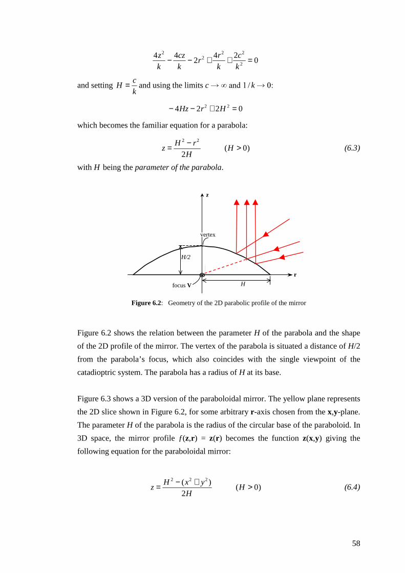
Figure 6.2: Geometry of the 2D parabolic profile of the mirror

Figure 6.2 shows the relation between the parameter H of the parabola and the shape

of the 2D profile of the mirror. The vertex of the parabola is situated a distance of H/2

from the parabola’s focus, which also coincides with the single viewpoint of the

catadioptric system. The parabola has a radius of H at its base.

Figure 6.3 shows a 3D version of the paraboloidal mirror. The yellow plane represents

the 2D slice shown in Figure 6.2, for some arbitrary r-axis chosen from the x,y-plane.

The parameter H of the parabola is the radius of the circular base of the paraboloid. In

3D space, the mirror profile ƒ(z,r) = z(r) becomes the function z(x,y) giving the

following equation for the paraboloidal mirror:

)0(2

)( 222

>+−= HH

yxHz (6.4)

H

H/2

r

z

vertex

focus V

59

Figure 6.3: Geometry of the 3D paraboloidal mirror

6.3 Resolution of the Paraboloidal Mirror

One of the main issues of catadioptric cameras is their non-uniform resolution.

[BAKE99] derived an equation for the resolution of catadioptric systems. In the case of

the paraboloidal mirror, the resolution of the catadioptric system equals that of the

conventional camera multiplied by a factor s that varies depending on the distance a

point is from the centre of the mirror.

222

2

+=H

rHs (6.5)

It can be easily seen from (6.5) that this factor ranges from H2/4 at the mirror’s centre,

to H2 at the boundary. This implies that the resolution changes by a factor of 4 across

the image. The highest resolution occurs at the mirror’s boundary.

Another way to see this is through the mirror’s angular gain [PAJD00]. This is shown

in Figure 6.4(a) below, where for constant image distances d1 = d2 = d3, the mirror

VXEWHQGV� DQJOHV� � � � )LJXUH�����E�� VKRZV� WKH� UHYHUVH�� IRU� FRQVWDQt angles 0°,

10°, 20°, up to 100° of elevation, the distance r from the image centre changes non-

uniformly.

Apart from the non-uniform resolution caused by the mirror’s shape (optical

resolution), there is also the problem of the rectangular pixel layout of the sensor

(acquisition sensor resolution). The number of pixels that coincide with the 10° circle

in Figure 6.4(b) are much less than the pixels on or near the 80° circle.

r

z

x

y

H

60

Figure 6.4: Non-uniform Mirror Gain of the paraboloidal mirror

Some applications try to correct for these problems by designing mirrors that have

constant angular gain, for example the equi-angular cameras of [OLLI99]. Or try to

achieve constant angular resolution on some known ground-plane with a fixed

distance from the camera [GASP02]. The system by [PAJD00] uses a sensor that has a

log-polar pixel layout to keep the pixel resolution constant across the image.

Unfortunately all these solutions are either limited to certain conditions (ground-plane

methods) or deviate from a single viewpoint.

6.4 Catadioptric Projective Geometry

Catadioptric cameras define an imaging process whereby incoming light that passes

through the single viewpoint is reflected by the mirror’s surface and is projected onto

the camera’s sensing device. Because of the single viewpoint constraint, this imaging

process defines a projection. In addition, this projection is not a perspective projection

due to the non-linearity introduced by the mirror’s curved surface – lines in the real

world are not necessarily projected as lines in the omnidirectional image.

[GEYE01] have examined the geometric nature of these projections and have shown

that the projection of a single-viewpoint catadioptric mirror is equivalent to a series of

projections via the sphere. For the paraboloidal mirror, its projection is equivalent to a

projection of world point to a sphere (centred on the single viewpoint, with radius H),

followed by a type of spherical projection from one of the poles of the sphere (called

a stereographic projection), as shown in Figure 6.5 below.

20° 50° 80° 100

d2d3

Hviewpoint Vr

z

d1

61

In addition, all the projections of the non-degenerate catadioptric systems are

equivalent and are a subset of the so-called quadratic projections [GEYE01].

Translating the point SP of Figure 6.5 along the z-axis towards point V, accounts for

the spherical projections equivalent to the projections of the other mirror types

(ellipsoid, hyperboloid, and planar mirror when SP = V). Therefore all these

projections are equivalent and one can ‘translate’ one model to another by re-

projection. This is done by [URBA00] to convert the omnidirectional images captured

by a hyperboloidal mirror to a parabolic projection model, as it is claimed that

working with epipolar lines is easier for the parabolic projection.

Figure 6.5: Equivalence of Parabolic Projection (green) to Stereographic Projection (red). (Without loss of generality, the image plane has been translated to the origin).

The series of Figures 6.6 to 6.7 show some of the characteristics of the parabolic

projection using the synthetic images generated in §3.4. The paraboloidal mirror has a

vertical field-of-view of 220º. Figure 6.6(a) shows that the horizon (the set of

vanishing points) is projected into a circle centred at the image centre.

In general, lines in the real world, under a parabolic projection, are mapped to conic

sections (circles, ellipses or lines) [GEYE01]. Figure 6.6(b) shows that vertical lines are

mapped to radial lines meeting at the image centre. On the other hand, non-vertical

lines are projected into circles, as shown in Figure 6.7(a). These obey the invariant: 222 4 fdR =−

H

r

z

world point

image point

SP

V

62

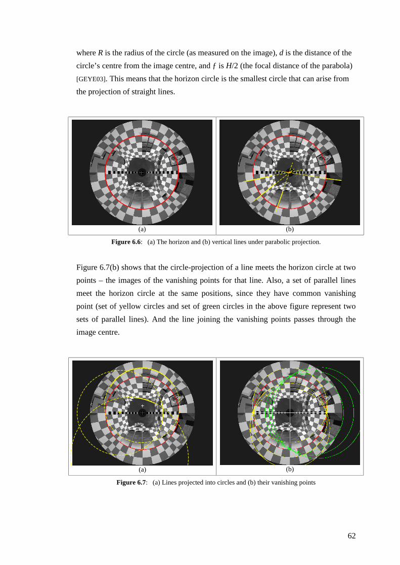
where R is the radius of the circle (as measured on the image), d is the distance of the

circle’s centre from the image centre, and ƒ is H/2 (the focal distance of the parabola)

[GEYE03]. This means that the horizon circle is the smallest circle that can arise from

the projection of straight lines.

(a) (b)

Figure 6.6: (a) The horizon and (b) vertical lines under parabolic projection.

Figure 6.7(b) shows that the circle-projection of a line meets the horizon circle at two

points – the images of the vanishing points for that line. Also, a set of parallel lines

meet the horizon circle at the same positions, since they have common vanishing

point (set of yellow circles and set of green circles in the above figure represent two

sets of parallel lines). And the line joining the vanishing points passes through the

image centre.

(a) (b)

Figure 6.7: (a) Lines projected into circles and (b) their vanishing points

6.5 Re-Projection Equations for a Paraboloidal Mirror.

The projection generated by the paraboloidal mirror is not a perspective projection as

it does not preserve lines, but maps them to conic sections. It also adds non-uniform

distortion effects to the imaging process. This creates ‘warped’ images such as those

of Figure 6.7, which are not suitable for human viewing. Therefore, to show a

geometrically-correct perspective image from an omnidirectional image, it must be

‘dewarped’ as mentioned in §2.5. Another reason for dewarping is that the bulk of

work in computer vision is based on perspective projection and rectilinear images.

Most of these methods are not suitable to be applied directly to the ‘raw’

omnidirectional images.

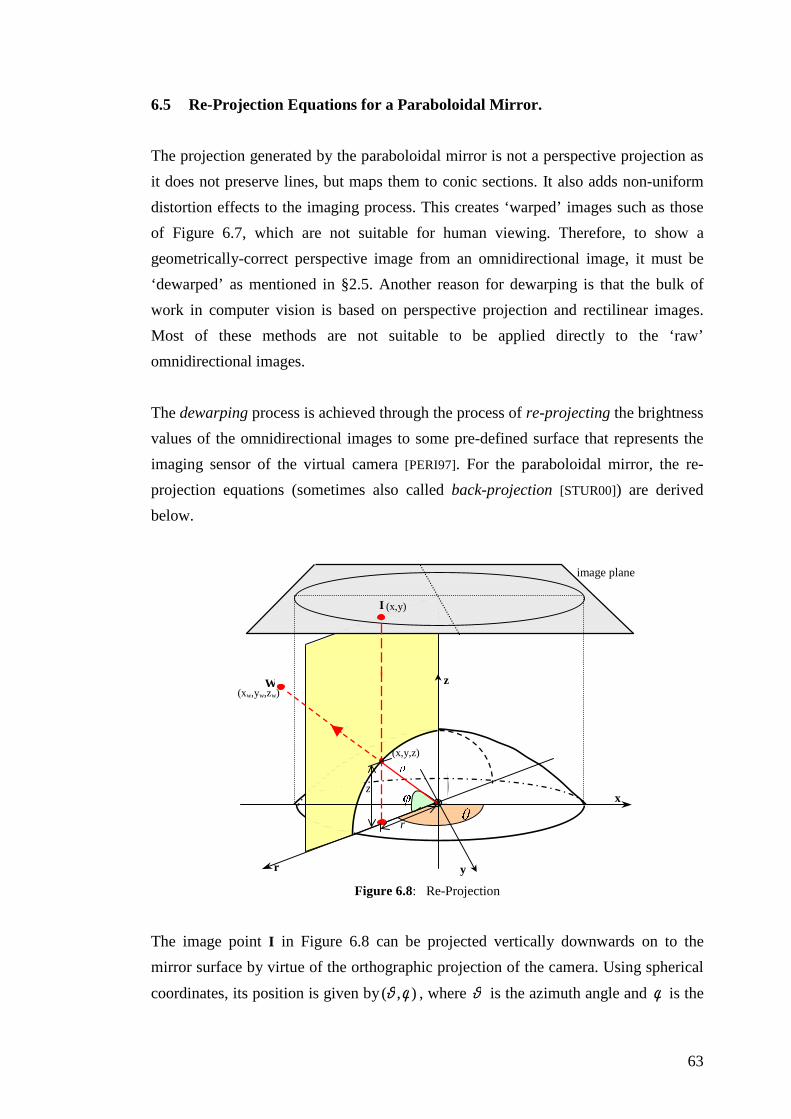
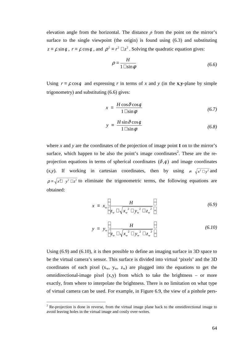
The dewarping process is achieved through the process of re-projecting the brightness

values of the omnidirectional images to some pre-defined surface that represents the

imaging sensor of the virtual camera [PERI97]. For the paraboloidal mirror, the re-

projection equations (sometimes also called back-projection [STUR00]) are derived

below.

Figure 6.8: Re-Projection

The image point I in Figure 6.8 can be projected vertically downwards on t

mirror surface by virtue of the orthographic projection of the camera. Using sph

coordinates, its position is given by ),( φϑ , where ϑ is the azimuth angle and φ

x

r y

zW

I (x,y)

r

z

(xw,yw,zw)

(x,y,z)

image plane

63

o the

erical

is the

64

elevation angle from the horizontal. The distance from the point on the mirror’s

surface to the single viewpoint (the origin) is found using (6.3) and substituting

φρ sin=z , φρ cos=r , and 222 zr +=ρ . Solving the quadratic equation gives:

φρ

sin1+= H

(6.6)

Using φρ cos=r and expressing r in terms of x and y (in the x,y-plane by simple

trigonometry) and substituting (6.6) gives:

φφϑ

sin1coscos

+= H

x (6.7)

φφϑ

sin1cossin

+= H

y (6.8)

where x and y are the coordinates of the projection of image point I on to the mirror’s

surface, which happen to be also the point’s image coordinates2. These are the re-

projection equations in terms of spherical coordinates ),( φϑ and image coordinates

(x,y). If working in cartesian coordinates, then by using 22 yxr += and

222 zyx ++=ρ to eliminate the trigonometric terms, the following equations are

obtained:

+++=

222wwww

wzyxz

Hxx (6.9)

+++=

222wwww

wzyxz

Hyy (6.10)

Using (6.9) and (6.10), it is then possible to define an imaging surface in 3D space to

be the virtual camera’s sensor. This surface is divided into virtual ‘pixels’ and the 3D

coordinates of each pixel (xw, yw, zw) are plugged into the equations to get the

omnidirectional-image pixel (x,y) from which to take the brightness – or more

exactly, from where to interpolate the brightness. There is no limitation on what type

of virtual camera can be used. For example, in Figure 6.9, the view of a pinhole pers-

2 Re-projection is done in reverse, from the virtual image plane back to the omnidirectional image to avoid leaving holes in the virtual image and costly over-writes.

pective camera and part of the view of a panoramic camera are shown. Other surfaces

that could be used are: a spherical surface (like in [THOM03]), a cubic surface (to be

used for example in CAVE systems3), special views for head-mounted displays, etc.

Figure 6.9: Generating Perspective and Panor

6.6 Implementation

6.6.1 Camera Models

The application written for this project, called OmniTr

virtual cameras – the perspective virtual camera and the

The perspective camera uses a rectilinear imaging surfac

uses a cylindrical surface for a 360° horizontal field-of-v

model chosen for the perspective camera and the camera

for altering its view.

The rectilinear surface of the perspective camera is by def

as its principal axis, and placed at a distance ƒc from the o

3 Cave Automatic Virtual Environment (CAVE) – a well-known virtua

I

W

image plane z

II

W(xw,yw,zw)

(x,y)(x,y)

(xw,yw,zw)

65

amic views

acking, uses two types of

panoramic virtual camera.

e while the panoramic one

iew. Figure 6.10 shows the

control parameters available

ault oriented with the x-axis

rigin (the viewpoint V). The

l reality system.

x

66

coordinates of the virtual pixels in the ‘image’ are measured in terms of vectors u and

v, with the origin set at the top-left corner of the image, in accordance with the normal

image convention. ƒc is the focal length of the perspective camera and is initially set

to be equal to the focal length of the paraboloidal mirror (that is, to ƒ = H/2).

(a) (b)

Figure 6.10: Virtual Perspective Camera Model. (a) Camera model; (b) Control Parameters

For camera control, the PTZ (pan-tilt-zoom) model was chosen. The pan angle is a

rotation around the z-axis, along the horizontal. Tilt defines the angle of elevation of

the camera4. The zoom factor is a multiplicative factor applied to the camera’s focal

length. If the zoom factor is 1, then the perspective camera has the same focal length

(and same magnification) as the omnidirectional camera. Larger (smaller) zoom

factors mean larger (smaller) magnifications than that of the omnidirectional image.

In addition to pan and tilt, a roll control parameter was also added. The roll angle

defines a rotation of the image plane around its principal point.5

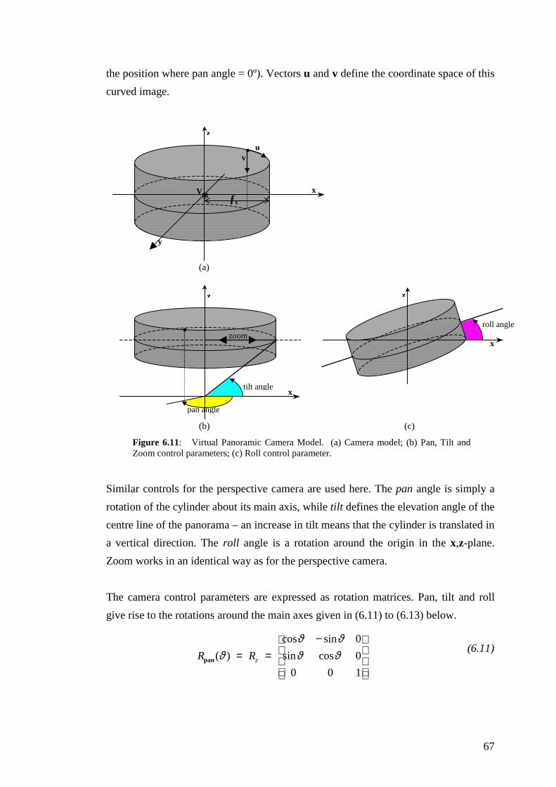
Figure 6.11 shows the camera model for the panoramic virtual camera. The image

surface for this kind of camera is a cylinder centred on the viewpoint and having a

radius of ƒc, the focal length of the panoramic camera (initially set to the focal length

of the paraboloidal mirror). The point chosen as the origin of the panoramic image is

at the top of the cylinder with an arbitrarily selected horizontal position (initially set to

4 These angles are specified with reference to the principal point – that is to the centre point of the image (where the principal axis crosses the image plane) and not to the origin of the image. 5 Note that the image plane remains perpendicular to the perspective camera’s principal axis (the line joining the viewpoint to the virtual image centre) under all of the above changes – as normally expected in the pinhole camera model. But it might be possible to tilt the image plane by some angle with respect to this axis. This particular model is used in real-life photography to correct for converging verticals, especially in architectural photography. In older times it was done through the use of camera bellows, but nowadays, special modern “tilt-shift” lenses are used [FREE93 pp. 150-151]. This and other special camera effects could be simulated through new virtual camera models.

x

z

V

uv

ƒc

x

z

V

tilt angle

pan angle

roll angle

zoom

67

the position where pan angle = 0º). Vectors u and v define the coordinate space of this

curved image.

(a)

(b) (c)

Figure 6.11: Virtual Panoramic Camera Model. (a) Camera model; (b) Pan, Tilt and Zoom control parameters; (c) Roll control parameter.

Similar controls for the perspective camera are used here. The pan angle is simply a

rotation of the cylinder about its main axis, while tilt defines the elevation angle of the

centre line of the panorama – an increase in tilt means that the cylinder is translated in

a vertical direction. The roll angle is a rotation around the origin in the x,z-plane.

Zoom works in an identical way as for the perspective camera.

The camera control parameters are expressed as rotation matrices. Pan, tilt and roll

give rise to the rotations around the main axes given in (6.11) to (6.13) below.

−==

100

0cossin

0sincos

)( ϑϑϑϑ

ϑ zRRpan

(6.11)

V

uv

ƒc

x

z

y

roll angle

x

z

x

pan angle

tilt angle

zoom

z

68

−==

ϑϑ

ϑϑϑ

cos0sin

010

sin0cos

)( yRRtilt

(6.12)

−==

ϑϑϑϑϑ

cossin0

sincos0

001

)( xRRroll

(6.13)

These are combined together into a transformation matrix R and this transformation

matrix is applied to the virtual camera in its default orientation (i.e. with pan, tilt, roll

equal to 0) to transform it to the new viewing directions.

rolltiltpan RRRR ⋅⋅= (6.14)

Zoom is used to generate the camera’s effective focal length using the equation

below. The zoom value for the OmniTracking application can take any value within

the range ×¼ to ×8.

/2factorzoomƒc H⋅= (6.15)

6.6.2 Re-Projection Optimisation

Equations (6.9) and (6.10) are quite expensive when used to generate video streams

for a number of virtual cameras in real-time, mainly because of the square-root

operation. For the OmniTracking application, a certain number of optimisations were

applied. First, most of the time the camera parameters stay constant, so the re-

projection can be calculated once and reused for successive frames until the camera’s

viewpoint changes. This is done by means of a look-up table (LUT). This approach is

similar to the geometric map method of [PERI97].

Given the coordinates (u,v) of a virtual pixel, its re-projected position in the

omnidirectional image is stored in reprojected_pos_table when the camera is

initialised or its viewpoint is updated. For the next frame, a simple lookup into

reprojected_pos_table[ (u,v) ] gives the position (x,y) in the omnidirectional image

from where the brightness is to be calculated. Interpolation is used to estimate the

brightness. By default, the interpolation method used is bicubic interpolation which

69

uses the neighbouring 16 pixels of (x,y). But the user can select one of two other

interpolations – bilinear interpolation, or simply nearest-neighbour interpolation –

which are quicker but produce poorer results.

In addition, a number of optimisations make the re-projection calculation faster.

Equations (6.9) and (6.10) contain 222www zyx ++ in their denominator. This term

stands for the distance d of the virtual pixel from the origin (the single viewpoint).

For the perspective camera model, the distance d can be split into two components –

the distance e of the pixel (xw,yw,zw) (or (u,v) in the virtual image coordinate frame)

from the principal point P within the imaging plane and the distance ƒc of the

principal point from the origin V (see Figure 6.12(a)). So the term 222www zyx ++ can

be expressed as 22 ƒce + which is equal to 222 ƒcvu ++ (see (6.16), (6.18) and

(6.19)). Both distance ƒc and distance e change only when the zoom factor changes.

So another lookup table can be used for this distance factor.

(a) (b)

Figure 6.12: Optimising the distance factor in the re-projection equations. (a) Optimis-ation for the perspective camera; (b) and for the panoramic camera.

For the panoramic camera model, the distance d is simpler. It can be split up into

distance ƒc (the radius of the cylinder) and distance e, the vertical distance of the pixel

from the principal circle P (see Figure 6.12(b)). The term 222www zyx ++ can be

expressed as 22 ƒce + which is equal to 220 ƒ)( cvv +− , where v0 is the vertical height

of the principal circle . Both distance ƒc and distance e change only when the zoom

factor changes. So another lookup table can be used for this distance factor. Because

z

xV

uv

P

d

(u,v)=(xw,yw,zw)

e

ƒc

u

d e

v

V x

z

ƒc

(u,v)

P

70

only the vertical component v is used in the calculation of e, then the lookup table is a

1-D array, indexed by v.

for perspective camera: 222 ƒcvud ++=

(6.16)

for panoramic camera: 22

0 ƒ)( cvvd +−=(6.17)

for both:

+

=dz

Hxx

ww (6.18)

+

=dz

Hyy

ww (6.19)

When a camera’s viewpoint changes, it is usually due to a change in one or a few of

the camera control parameters, while the rest of the parameters stay fixed. Figure 6.13

(next page) shows how this is used to skip unnecessary calculations and make the

calculation of the re-projection lookup tables faster. Separate rotation matrices (for

pan, tilt, roll) are also saved and changed only when the corresponding angle changes.

6.6.3 Interactive Control

The OmniTracking application’s graphical user interface (GUI) allows the user to

open a number of virtual camera video streams (perspective and/or panoramic) at run-

time and to interactively control each one of them. In addition, when running in

camera auto-track mode, a number of cameras could be used to automatically follow

targets as they are detected and move across the field-of-view of the omnidirectional

sensor (more details about this functionality in §12).

71

Figure 6.13: Algorithm for calculating the Re-Projection Look-Up Table

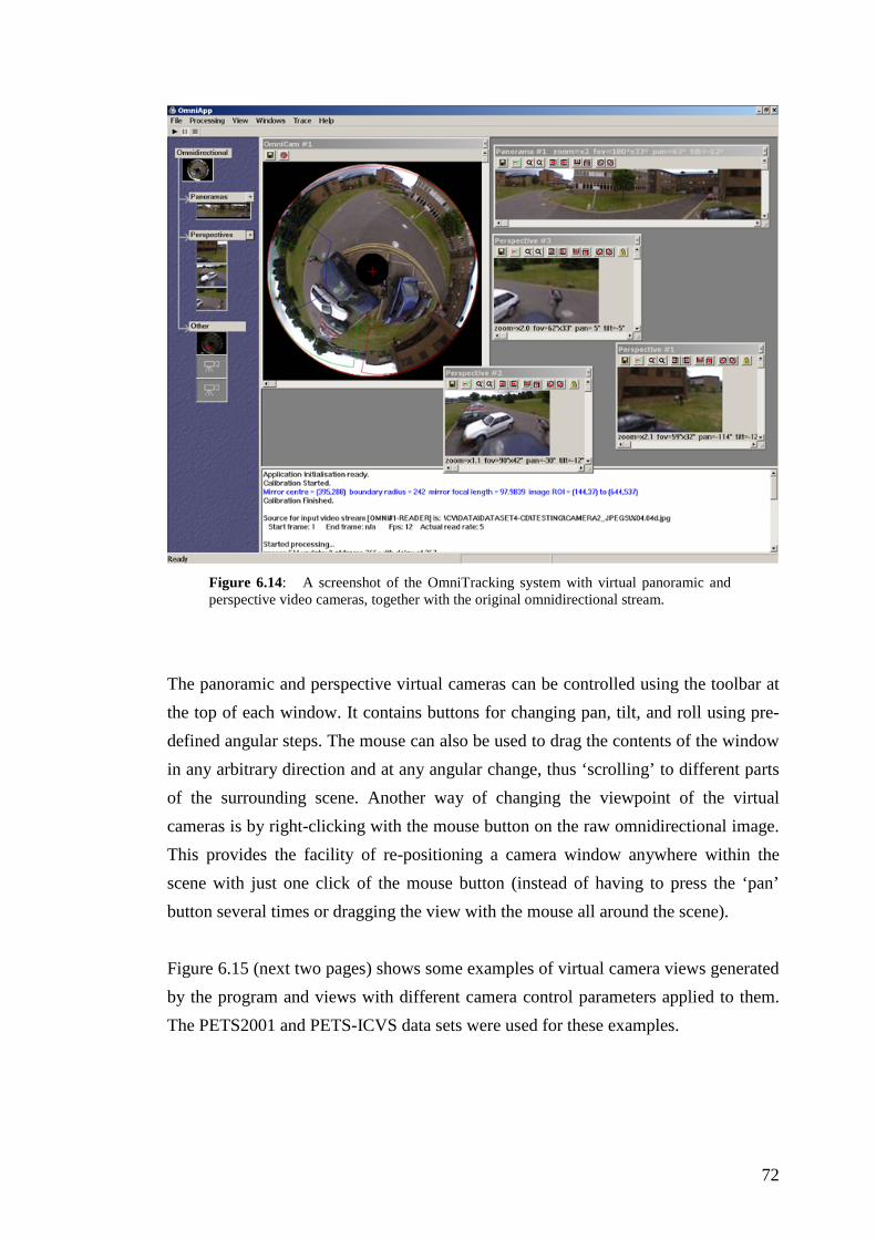
A screenshot of the application is shown in Figure 6.14. A problem with many image-

based programs that use free-floating windows is that when many windows are open,

the screen can become cluttered, windows are ‘lost’ when hidden by others, etc. The

icon toolbar on the left attempts to make things a bit more manageable. It provides a

fast access mechanism to activate/show the windows on screen, and a way of allowing

the user to see at a glance how many windows are currently open and what they

contain. It can also be used to create more panoramic or perspective camera views.

Apply transformation matrix R to the pixels, and compute new reprojected_pos_table using (6.18) and (6.19). The value for d is looked up in distance_table.

recalculate transformation matrix R using (6.14)

clear and re-allocate memory for the lookup tables reprojected_pos_table and distance_table

has virtual image size changed?

recalculate the distance of each pixel and store in distance_table using (6.16) or (6.17).

has zoom factor changed?

has pan changed? recalculate rotation matrix Rpan using (6.11)

has tilt changed? recalculate rotation matrix Rtilt using (6.12)

has tilt, pan or roll changed?

recalculate rotation matrix Rroll using (6.13) has roll changed?

72

Figure 6.14: A screenshot of the OmniTracking system with virtual panoramic and perspective video cameras, together with the original omnidirectional stream.

The panoramic and perspective virtual cameras can be controlled using the toolbar at

the top of each window. It contains buttons for changing pan, tilt, and roll using pre-

defined angular steps. The mouse can also be used to drag the contents of the window

in any arbitrary direction and at any angular change, thus ‘scrolling’ to different parts

of the surrounding scene. Another way of changing the viewpoint of the virtual

cameras is by right-clicking with the mouse button on the raw omnidirectional image.

This provides the facility of re-positioning a camera window anywhere within the

scene with just one click of the mouse button (instead of having to press the ‘pan’

button several times or dragging the view with the mouse all around the scene).

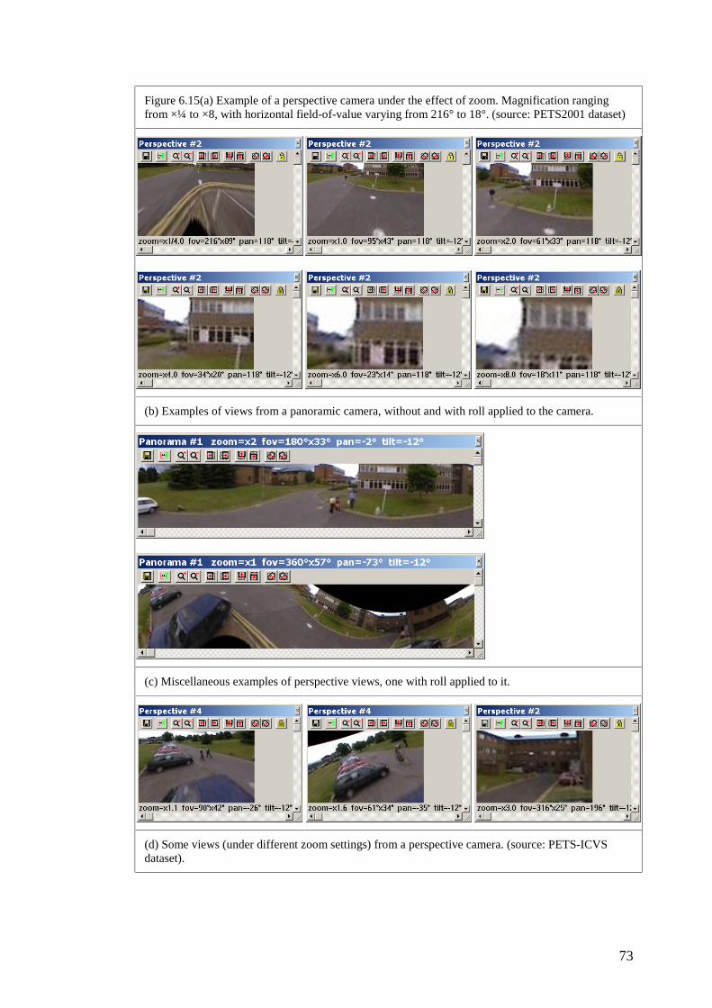
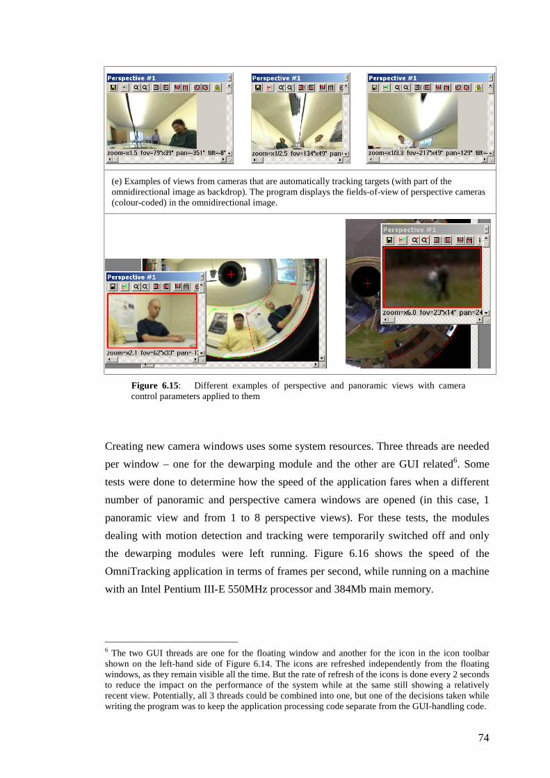
Figure 6.15 (next two pages) shows some examples of virtual camera views generated

by the program and views with different camera control parameters applied to them.

The PETS2001 and PETS-ICVS data sets were used for these examples.

73

Figure 6.15(a) Example of a perspective camera under the effect of zoom. Magnification ranging from ×¼ to ×8, with horizontal field-of-value varying from 216° to 18°. (source: PETS2001 dataset)

(b) Examples of views from a panoramic camera, without and with roll applied to the camera.

(c) Miscellaneous examples of perspective views, one with roll applied to it.

(d) Some views (under different zoom settings) from a perspective camera. (source: PETS-ICVS dataset).

74

(e) Examples of views from cameras that are automatically tracking targets (with part of the omnidirectional image as backdrop). The program displays the fields-of-view of perspective cameras (colour-coded) in the omnidirectional image.

Figure 6.15: Different examples of perspective and panoramic views with camera control parameters applied to them

Creating new camera windows uses some system resources. Three threads are needed

per window – one for the dewarping module and the other are GUI related6. Some

tests were done to determine how the speed of the application fares when a different

number of panoramic and perspective camera windows are opened (in this case, 1

panoramic view and from 1 to 8 perspective views). For these tests, the modules

dealing with motion detection and tracking were temporarily switched off and only

the dewarping modules were left running. Figure 6.16 shows the speed of the

OmniTracking application in terms of frames per second, while running on a machine

with an Intel Pentium III-E 550MHz processor and 384Mb main memory.

6 The two GUI threads are one for the floating window and another for the icon in the icon toolbar shown on the left-hand side of Figure 6.14. The icons are refreshed independently from the floating windows, as they remain visible all the time. But the rate of refresh of the icons is done every 2 seconds to reduce the impact on the performance of the system while at the same still showing a relatively recent view. Potentially, all 3 threads could be combined into one, but one of the decisions taken while writing the program was to keep the application processing code separate from the GUI-handling code.

75

0

5

10

15

20

25

30

35

number of virtual camerasfr

ames

per

sec

on

d

Figure 6.16: Performance of generating virtual camera views by the OmniTracking program

Some possible future enhancements that can be added to OmniTracking’s dewarping

module are:

• Allowing the dewarper to combine two omnidirectional video streams to

generate perspective and panoramic camera views. This would handle the

back-to-back paraboloidal mirror systems mentioned in §3.3.

• Because of the limited resolution of omnidirectional systems, the dewarper

module could make use of additional video streams from standard cameras to

fuse together the dewarped low-res omnidirectional image with any high-res

views from standard cameras that happen to be pointed in that particular

direction. [HALL01] uses this method to produce a so-called resolution on

demand system.

6.7 Conclusion

This chapter described the geometry of single-viewpoint catadioptric systems. In the

first section, the general single-viewpoint mirror equations were introduced and from

these, the equations for the paraboloidal mirror were derived. This was followed by a

discussion on how world lines and points are mapped under the parabolic projection

of the mirror. Using the mirror equations and knowledge about the parabolic

projection, the process of re-projection was introduced and it was shown how this can

be used to generate virtual views. Two virtual camera types were described – the

perspective camera and the panoramic camera, and a camera control mechanism was

introduced to allow the user to interactively control the cameras. The chapter finished

with a sample of virtual images generated by the OmniTracking application.

2 3 4 5 6 7 8 9