81

CHAPTER 6

ADAPTIVE HYSTERESIS CURRENT CONTROL OF

DC-AC INVERTER IN A GRID CONNECTED PV SYSTEM

6.1 INTRODUCTION

The previous chapters have discussed the development of the

MPPT algorithm and the control of the DC-DC converter in a standalone PV

system. A grid-connected PV system is composed of a photovoltaic array,

DC-DC converter, DC link capacitor, single phase DC-AC inverter, filter

inductor, power grid, and non-linear load. The grid interconnection of a PV

power generation system has the advantage of more effective utilization of the

generated power. The Grid interconnection of PV systems is accomplished

through the inverter. The Grid-connected inverter is the critical interface of a

photovoltaic array connected with the power grid. Pulse width modulation

(PWM) is the most popular control technique in voltage-source inverters.

Compared to the PWM converters, the current-controlled PWM has several

advantages. It has lesser distortion and lower harmonic noise. This chapter

deals with the development of adaptive hysteresis current control techniques

for the DC-AC inverter, in order to provide a constant switching frequency

with less harmonic content. The simulation results obtained, using the

proposed current control technique, are presented. The hardware

implementation of the proposed inverter current control algorithms using

Xilinx spartran-3 FPGA, is also presented.

82

6.2 GRID CONNECTED SOLAR PV SYSTEM

(a)

(b)

Figure 6.1 (a) Block diagram representation of a grid connected PV system, (b) Schematic diagram of the grid connected PV system

Figure 6.1(a) shows the grid connected PV system. Figure 6.1(b)

shows the schematic diagram of a grid connected PV system along with

various controllers. The presented system consists of PV modules, a DC-DC

converter, DC link capacitor, DC-AC converter, MPPT controller, Adaptive

hysteresis current controller, PWM controller, and a grid. The solar

photovoltaic array produces electricity when the photon of sunlight strikes the

PV cell array. The output of the PV panel is directly connected to the DC-DC

boost converter, to step up the DC output of the photovoltaic panel and to

perform the MPPT. The conventional perturb and observe MPPT controller is

used in this case, the details of which are given in Appendix 2. Then it is fed

83

to an inverter through a DC link capacitor. The inverter converts DC into AC

power at the desired voltage and frequency, to perform the output current

control. One of the important in the development of a single phase inverter for

PV application is the DC-link capacitor. The DC link contains power

pulsation, so that the capacitor should be connected to absorb this pulsating

power to reduce the DC-link voltage ripple. The value of the DC-link

capacitor is calculated by the equation (6.1).

rippledcdc VV

PCω2

=

(6.1)

where P is the Power, ω is the output AC voltage frequency, Vdc is the

nominal DC voltage and Vripple is the maximum allowed ripple voltage.

6.3. MODEL OF AN INVERTER

The model of the DC-AC converter is needed to simulate the circuit

and to analyze its behavior. Figure 6.2(a) shows the circuit diagram of a

DC-AC single phase full bridge Inverter.

(a)

84

(b)

Figure 6.2. (a) Circuit diagram of a DC-AC inverter, (b) PWM signal for a DC-AC inverter

The PV inverter is designed for 230V, 50 Hz. The DC voltage

which is obtained from the converter output is given to the inverter,

for converting it to a smooth sinusoidal waveform. An inductor current

flowing through filter, and load voltage are considered as state variable. The

state equations with S1 and S3 ON (d interval) and S1 and S3 OFF (1-d

interval) are expressed as:

SLL v

Lv

RCi

Cv

Ldt

di 111100 +−+−= (6.2)

SLL v

Lv

RCi

Cv

Ldt

di 111100 −−+−= (6.3)

The basic operation of the dc–ac full-bridge switching converter is

that each pair of switches, S1–S3 and S2–S4, are operated alternately for each

switching period with their duty cycle (d). The duty cycle (d) is a ratio of an

ON time (ton) to a switching period (T), d= ton /TS= ton fs, as shown in

Figure 6.2 (b).

85

6.4 CONTROL OF THE SOLAR PV INVERTER

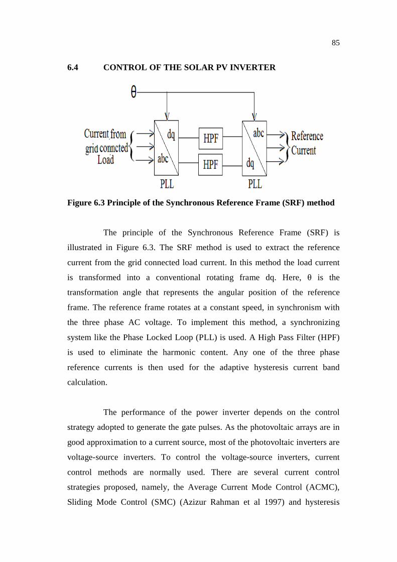
Figure 6.3 Principle of the Synchronous Reference Frame (SRF) method

The principle of the Synchronous Reference Frame (SRF) is

illustrated in Figure 6.3. The SRF method is used to extract the reference

current from the grid connected load current. In this method the load current

is transformed into a conventional rotating frame dq. Here, θ is the

transformation angle that represents the angular position of the reference

frame. The reference frame rotates at a constant speed, in synchronism with

the three phase AC voltage. To implement this method, a synchronizing

system like the Phase Locked Loop (PLL) is used. A High Pass Filter (HPF)

is used to eliminate the harmonic content. Any one of the three phase

reference currents is then used for the adaptive hysteresis current band

calculation.

The performance of the power inverter depends on the control

strategy adopted to generate the gate pulses. As the photovoltaic arrays are in

good approximation to a current source, most of the photovoltaic inverters are

voltage-source inverters. To control the voltage-source inverters, current

control methods are normally used. There are several current control

strategies proposed, namely, the Average Current Mode Control (ACMC),

Sliding Mode Control (SMC) (Azizur Rahman et al 1997) and hysteresis

86

control (Anushuman Shukla et al 2007). Among the various current control

techniques, hysteresis control is the most popular one for a voltage source

inverter. The conventional Hysteresis controller is a fixed hysteresis band

controller. This is very simple, has a robust current control performance with

good stability, very fast response, an inherent ability to control peak current,

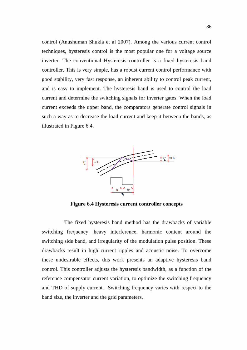
and is easy to implement. The hysteresis band is used to control the load

current and determine the switching signals for inverter gates. When the load

current exceeds the upper band, the comparators generate control signals in

such a way as to decrease the load current and keep it between the bands, as

illustrated in Figure 6.4.

Figure 6.4 Hysteresis current controller concepts

The fixed hysteresis band method has the drawbacks of variable

switching frequency, heavy interference, harmonic content around the

switching side band, and irregularity of the modulation pulse position. These

drawbacks result in high current ripples and acoustic noise. To overcome

these undesirable effects, this work presents an adaptive hysteresis band

control. This controller adjusts the hysteresis bandwidth, as a function of the

reference compensator current variation, to optimize the switching frequency

and THD of supply current. Switching frequency varies with respect to the

band size, the inverter and the grid parameters.

87

Figure 6.5 Principle of the adaptive hysteresis current controller concept

Figure 6.5 shows the concept of the adaptive hysteresis current

controller where the ascendant and descendant slopes of the inverter reference

current compensator are produced by imposing voltage stresses +Vdc & -Vdc

on an inductor, which connects the inverter to the grid.

The equation for the hysteresis bandwidth is given below as:

(Xunjiang Dai, Qin Chao, 2009):

)](1

1)[(2

1

dt

diLV

Vdt

diLV

LfHB ref

Sdc

refS

S

+−+= (6.4)

Equation (6.4) defines the hysteresis band that depends on the

system parameters. By substituting the desired switching frequency, the

hysteresis band value is obtained. Hence, the algorithm that adaptively adjusts

the hysteresis band width based upon electrical parameters, with the purpose

of maintaining constant switching frequency, is known as the adaptive

hysteresis current controller.

88

6.5 SIMULATION OF A PV SYSTEM WITH ADAPTIVE

HYSTERESIS CURRENT CONTROL

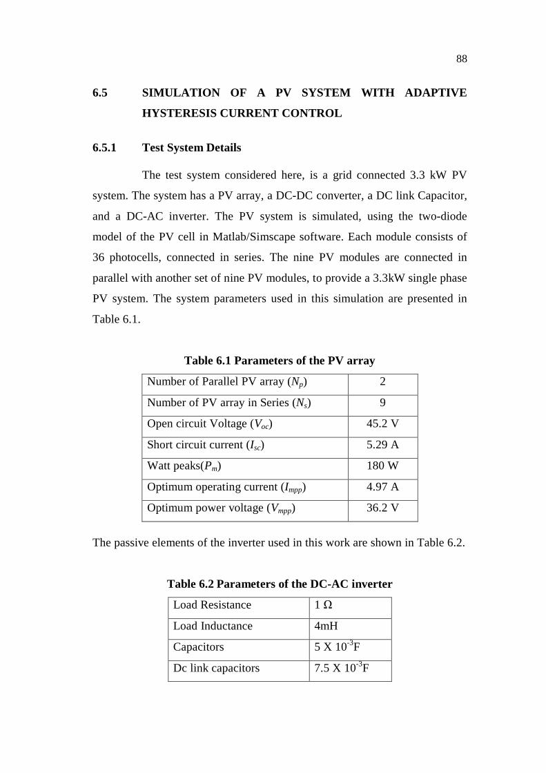
6.5.1 Test System Details

The test system considered here, is a grid connected 3.3 kW PV

system. The system has a PV array, a DC-DC converter, a DC link Capacitor,

and a DC-AC inverter. The PV system is simulated, using the two-diode

model of the PV cell in Matlab/Simscape software. Each module consists of

36 photocells, connected in series. The nine PV modules are connected in

parallel with another set of nine PV modules, to provide a 3.3kW single phase

PV system. The system parameters used in this simulation are presented in

Table 6.1.

Table 6.1 Parameters of the PV array

Number of Parallel PV array (Np) 2

Number of PV array in Series (Ns) 9

Open circuit Voltage (Voc) 45.2 V

Short circuit current (Isc) 5.29 A

Watt peaks(Pm) 180 W

Optimum operating current (Impp) 4.97 A

Optimum power voltage (Vmpp) 36.2 V

The passive elements of the inverter used in this work are shown in Table 6.2.

Table 6.2 Parameters of the DC-AC inverter

Load Resistance 1 Ω

Load Inductance 4mH

Capacitors 5 X 10-3F

Dc link capacitors 7.5 X 10-3F

89

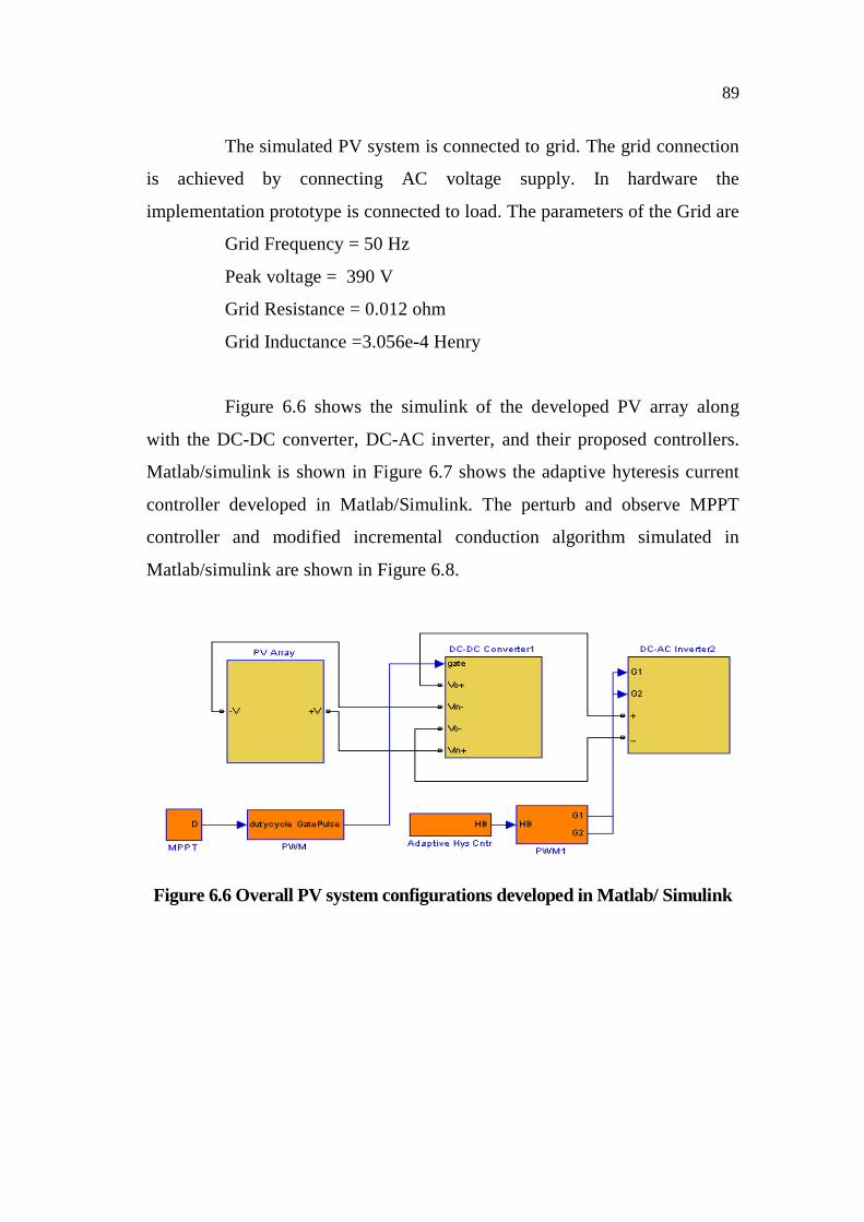
The simulated PV system is connected to grid. The grid connection

is achieved by connecting AC voltage supply. In hardware the

implementation prototype is connected to load. The parameters of the Grid are

Grid Frequency = 50 Hz

Peak voltage = 390 V

Grid Resistance = 0.012 ohm

Grid Inductance =3.056e-4 Henry

Figure 6.6 shows the simulink of the developed PV array along

with the DC-DC converter, DC-AC inverter, and their proposed controllers.

Matlab/simulink is shown in Figure 6.7 shows the adaptive hyteresis current

controller developed in Matlab/Simulink. The perturb and observe MPPT

controller and modified incremental conduction algorithm simulated in

Matlab/simulink are shown in Figure 6.8.

Figure 6.6 Overall PV system configurations developed in Matlab/ Simulink

90

Figure 6.7. Adaptive hysteresis current controller developed in Matlab/ Simulink

(a)

91

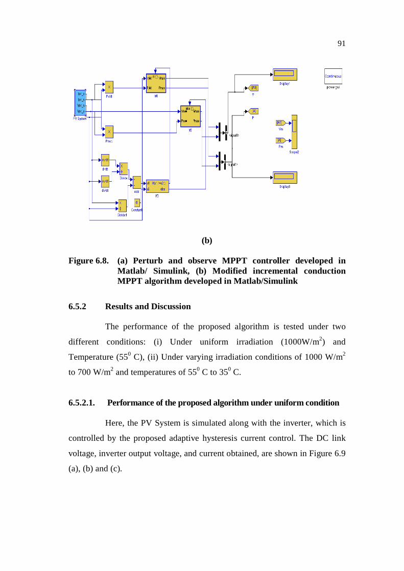
(b)

Figure 6.8. (a) Perturb and observe MPPT controller developed in Matlab/ Simulink, (b) Modified incremental conduction MPPT algorithm developed in Matlab/Simulink

6.5.2 Results and Discussion

The performance of the proposed algorithm is tested under two

different conditions: (i) Under uniform irradiation (1000W/m2) and

Temperature (550 C), (ii) Under varying irradiation conditions of 1000 W/m2

to 700 W/m2 and temperatures of 550 C to 350 C.

6.5.2.1. Performance of the proposed algorithm under uniform condition

Here, the PV System is simulated along with the inverter, which is

controlled by the proposed adaptive hysteresis current control. The DC link

voltage, inverter output voltage, and current obtained, are shown in Figure 6.9

(a), (b) and (c).

92

Figure 6.9 (a) DC link voltage, (b) Inverter Current and (c) Inverter voltage

The THD and switching frequency in this case are shown in

Figure 6.10 (a) and (b).

93

(a)

(b)

Figure 6.10 (a) THD level of the adaptive hysteresis controller of the photovoltaic inverter, (b) Switching frequency of the adaptive hysteresis controller of the photovoltaic inverter

The THD in this case is 3.14%. Also, the modulation frequency is

maintained constant at 5 kHz, as shown in Figure 6.10. The current has a low

total harmonic distortion, and a constant switching frequency.

For comparison, the inverter was controlled using a sinusoidal

PWM, and fixed hysteresis current control techniques. The load current

harmonic spectrum and its switching frequency of sinusoidal PWM controlled

inverter are shown in Figure 6.11 (a) and (b). The total harmonic distortion

(THD) in this case is 7.81%. Also, it is observed from Figure 6.11, that the

switching frequency varies over a wide range. The sine PWM which is

94

otherwise called as carrier based PWM technique compares low frequency

sine (modulated) wave with the high frequency triangular (carrier) wave. This

generates varying pulse width which leads to variable switching frequency.

Figure 6.12. shows the output current, harmonic current and the switching

frequency, in the case of the fixed hysteresis band controller. The fixed

hysteresis control method builds fixed band for current tracking, hence the

switching speed becomes variable which leads to variable switching

frequency. Table 6.3 gives the average switching frequency, and the

percentage THD values of load current with different techniques. From this

table it is observed, that the switching frequency is constant and THD is

minimized in the proposed technique.

(a)

(b)

Figure 6.11 (a) THD of the photovoltaic inverter sinusoidal PWM, (b) Switching frequency of the photovoltaic inverter sinusoidal PWM

95

Figure 6.12 (a) THD level of the fixed hysteresis controller of the photovoltaic inverter, (b). Switching frequency of the fixed hysteresis controller of the photovoltaic inverter

Table 6.3 Results of various techniques

Current control Technique THD % Average switching frequency

(kHz)

Adaptive Hysteresis band 3.14 5

Fixed Hysteresis band 6.93 2.26

Sinusoidal PWM 7.81 3.28

According to the IEEE 519-1992 standard, the THD value of the

voltages should not exceed 5%. Table 6.3 shows that the THD value of the

output voltage is acceptable by the IEEE standard.

6.5.2.2 Robustness of the proposed algorithm to irradiation and

temperature changes

In order to verify the robustness of the proposed algorithm, the

input of the PV array solar irradiation and temperature are varied, to represent

96

the varying atmospheric conditions. It is assumed that the PV array initially

receives a uniform irradiation of 1000 W/m2 and the temperature is 55oC. A

step change in the irradiation level (from 1000 and 700 W/m2) and

temperature (from 55oC to 35oC) are applied at t = 0.3 s. The DC link voltage

and inverter current waveform for this case, are shown in Figure 6.13 (a-d).

97

Figure 6.13 (a) Simulation of the varying solar irradiation according to time, (b) Simulation of the varying solar temperature according to time, (c) Response of the DC link voltage with the proposed MPPT algorithm, (d) Response of the inverter current P&O and the proposed MPPT algorithm, (e) Response of the switching frequency of the PV inverter

From Figure 6.13, it is observed that up to t=0.3 s, the DC link

voltage is maintained at 400 V. The changing irradiation and temperature (at

t=0.3 s) produce oscillations in the dc link voltage initially; after a short

moment it retains the voltage of 400 V. But it is observed that the sudden

partial shading effect at t=0.3s decreases the inverter current. The switching

frequency in this case is almost constant, as in the case of a uniform

atmospheric condition.

6.6. FPGA REALIZATION OF THE PROPOSED INVERTER

CONTROL

To verify the performance of the adaptive hysteresis current

controller, experimental studies were conducted on the prototype of the power

conditioning system. The developed prototype is composed of a single phase

inverter, and a Spartan 3 xilinx FPGA development board. Figure. 6.14 show

the experimental setup.

98

Figure. 6.14 Experimental setup

The proposed algorithm is executed in FPGA and its output gate

pulses are shown in Figure 6.15 (a). The snapshot of the input and output port

assignment is also depicted in Figure 6.15 (b).

(a)

(b)

Figure 6.15 (a) FPGA generated gate pulses, (b) Input, output port assignment snap-shot

Spartan-3 xilinx FPGA Single Phase Inverter

99

The output waveform of the voltage and current is shown in Figure 6.16.

(a)

(b)

Voltage=20v/div, Current=500mA/div, Time=5ms/div, THD=5.59%

Figure 6.16 (a) Inverter output voltage (upper) and current (lower) waveform, (b) THD of the inverter output voltage waveform

The THD of the output voltage is 5.59%. The THD in the

experimental waveform is higher, when compared to the simulated one, which

can be further reduced by a more accurate selection of the LC filters used.

100

6.7 CONCLUSION

This chapter has presented an inverter controller for the grid

connected PV system. The adaptive hysteresis current controller is used to

control the DC-AC inverter. The proposed algorithm for the inverter

controller has been tested on a 3.3 kW PV array of a grid connected PV

system in Matlab/ simulink simulation and FPGA based hardware prototype.

Based on the observation of the simulation and experimental results, the

developed algorithm is found to be very efficient, in terms of the constant

switching frequency and lesser THD value. The proposed current control

algorithm overcomes the difficulties and limitations, especially the variable

switching frequency, encountered by conventional approaches.