CHAPTER 6 · 6. FOB shipping point means that ownership of goods in transit passes to the buyer...
78
Copyright © 2013 John Wiley & Sons, Inc. Weygandt Financial, IFRS, 2/e, Solution’s Manual (For Instructor Use Only) 6-1 CHAPTER 6 Inventories ASSIGNMENT CLASSIFICATION TABLE Learning Objectives Questions Brief Exercises Do It! Exercises A Problems B Problems 1. Describe the steps in determining inventory quantities. 1, 2, 3, 4, 5, 6 1 1 1, 2 1A 1B 2. Explain the accounting for inventories and apply the inventory cost flow methods. 7, 8, 9, 10 2, 3 2 3, 4, 5, 6, 7 2A, 3A, 4A, 5A, 6A, 7A 2B, 3B, 4B, 5B, 6B, 7B 3. Explain the financial effects of the inventory cost flow assumptions. 4 3, 6, 7 2A, 3A, 4A, 5A, 6A, 7A 2B, 3B, 4B, 5B, 6B, 7B 4. Explain the lower-of- cost-or-net realizable value basis of accounting for inventories. 11, 12, 13 5 3 8, 9 5. Indicate the effects of inventory errors on the financial statements. 14 6 10, 11 6. Compute and interpret the inventory turnover ratio. 15, 16 7 4 12, 13 *7. Apply the inventory cost flow methods to perpetual inventory records. 17 8 14, 15, 16 8A, 9A 8B, 9B *8. Describe the two methods of estimating inventories. 18, 19, 20, 21 9, 10 17, 18, 19 10A, 11A 10B, 11B *9. Apply the LIFO inventory costing method 22, 23, 24 11 20, 21 12A 12B *Note: All asterisked Questions, Exercises, and Problems relate to material contained in the appendices to the chapter.
Transcript of CHAPTER 6 · 6. FOB shipping point means that ownership of goods in transit passes to the buyer...

Copyright © 2013 John Wiley & Sons, Inc. Weygandt Financial, IFRS, 2/e, Solution’s Manual (For Instructor Use Only) 6-1
CHAPTER 6 Inventories
ASSIGNMENT CLASSIFICATION TABLE Learning Objectives
Questions
Brief Exercises
Do It!
Exercises
A Problems
B Problems
1. Describe the steps in
determining inventory quantities.
1, 2, 3, 4, 5, 6
1 1 1, 2 1A 1B
2. Explain the accounting
for inventories and apply the inventory cost flow methods.
7, 8, 9, 10
2, 3 2 3, 4, 5, 6, 7
2A, 3A, 4A, 5A, 6A, 7A
2B, 3B, 4B, 5B, 6B, 7B
3. Explain the financial
effects of the inventory cost flow assumptions.
4 3, 6, 7 2A, 3A, 4A, 5A, 6A, 7A
2B, 3B, 4B, 5B, 6B, 7B
4. Explain the lower-of-
cost-or-net realizable value basis of accounting for inventories.
11, 12, 13 5 3 8, 9
5. Indicate the effects of
inventory errors on the financial statements.
14 6 10, 11
6. Compute and interpret
the inventory turnover ratio.
15, 16 7 4 12, 13
*7. Apply the inventory
cost flow methods to perpetual inventory records.
17 8 14, 15, 16 8A, 9A 8B, 9B
*8. Describe the two
methods of estimating inventories.
18, 19, 20, 21
9, 10 17, 18, 19 10A, 11A 10B, 11B
*9. Apply the LIFO
inventory costing method
22, 23, 24 11 20, 21 12A 12B
*Note: All asterisked Questions, Exercises, and Problems relate to material contained in the appendices to the chapter.

6-2 Copyright © 2013 John Wiley & Sons, Inc. Weygandt Financial, IFRS, 2/e, Solution’s Manual (For Instructor Use Only)
ASSIGNMENT CHARACTERISTICS TABLE Problem Number
Description
Difficulty Level
Time Allotted (min.)
1A Determine items and amounts to be recorded in inventory. Moderate 15–20
2A Determine cost of goods sold and ending inventory using
FIFO and average-cost with analysis. Simple 30–40
3A Determine cost of goods sold and ending inventory using
FIFO and average-cost with analysis. Simple 30–40
4A Compute ending inventory, prepare income statements, and
answer questions using FIFO and average-cost. Moderate 30–40
5A Calculate ending inventory, cost of goods sold, gross profit,
and gross profit rate under periodic method; compare results.
Moderate 30–40
6A Compare specific identification, FIFO, and average-cost
under periodic method; use cost flow assumption to influence earnings.
Moderate 20–30
7A Compute ending inventory, prepare income statements, and
answer questions using FIFO and average-cost. Moderate 30–40
*8A Calculate cost of goods sold and ending inventory for
FIFO and moving-average cost under the perpetual system; compare gross profit under each assumption.
Moderate 30–40
*9A Determine ending inventory under a perpetual inventory
system. Moderate 40–50
*10A Estimate inventory loss using gross profit method. Moderate 30–40
*11A Compute ending inventory using retail method. Moderate 20–30
*12A Apply the LIFO cost method (periodic) Simple 10–15
1B Determine items and amounts to be recorded in inventory. Moderate 15–20
2B Determine cost of goods sold and ending inventory using
FIFO and average-cost with analysis. Simple 30–40
3B Determine cost of goods sold and ending inventory using
FIFO and average-cost with analysis. Simple 30–40
4B Compute ending inventory, prepare income statements, and
answer questions using FIFO and average-cost. Moderate 30–40
5B Calculate ending inventory, cost of goods sold, gross profit,
and gross profit rate under periodic method; compare results.
Moderate 30–40
6B Compare specific identification, FIFO, and average-cost
under periodic method; use cost flow assumption to justify price increase.
Moderate 20–30

Copyright © 2013 John Wiley & Sons, Inc. Weygandt Financial, IFRS, 2/e, Solution’s Manual (For Instructor Use Only) 6-3
ASSIGNMENT CHARACTERISTICS TABLE (Continued) Problem Number
Description
DifficultyLevel
Time Allotted (min.)
7B Compute ending inventory, prepare income statements, and
answer questions using FIFO and average-cost. Moderate 30–40
*8B Calculate cost of goods sold and ending inventory under
FIFO, and moving-average cost, under the perpetual system; compare gross profit under each assumption.
Moderate 30–40
*9B Determine ending inventory under a perpetual inventory
system. Moderate 40–50
*10B Compute gross profit rate and inventory loss using gross
profit method. Moderate 30–40
*11B Compute ending inventory using retail method. Moderate 20–30
*12B Apply the LIFO cost method (periodic) Simple 10–15

6-4 Copyright © 2013 John Wiley & Sons, Inc. Weygandt Financial, IFRS, 2/e, Solution’s Manual (For Instructor Use Only)
WEYGANDT FINANCIAL ACCOUNTING, IFRS Edition, 2e CHAPTER 6
INVENTORIES
Number LO BT Difficulty Time (min.) BE1 1 C Simple 4–6 BE2 2 K Simple 2–4 BE3 2 AP Simple 4–6 BE4 3 C Simple 2–4 BE5 4 AP Simple 2–4 BE6 5 AN Moderate 6–8 BE7 6 AP Simple 4–6 BE8 *7 AP Simple 4–6 BE9 *8 AP Simple 4–6 BE10 *8 AP Simple 8–10 BE11 *9 AP Simple 4–6 DI1 1 AN Simple 4–6 DI2 2 AP Simple 6–8 DI3 4 AP Simple 6–8 DI4 6 AP Simple 4–6 EX1 1 AN Simple 4–6 EX2 1 AN Simple 6–8 EX3 2, 3 AP, E Moderate 6–8 EX4 2 AP, E Simple 8–10 EX5 2 AP Simple 6–8 EX6 2, 3 AP Simple 8–10 EX7 2, 3 AP Simple 8–10 EX8 4 AP Simple 6–8 EX9 4 AP Simple 6–8 EX10 5 AN Simple 4–6 EX11 5 AN Simple 6–8 EX12 6 AP Simple 10–12 EX13 6 AP Simple 10–12 EX14 *7 AP Simple 8–10
EX15 *7 AP, E Moderate 8–10
EX16 *7 AP, E Moderate 12–15

Copyright © 2013 John Wiley & Sons, Inc. Weygandt Financial, IFRS, 2/e, Solution’s Manual (For Instructor Use Only) 6-5
INVENTORIES (Continued)
Number LO BT Difficulty Time (min.) EX17 *8 AP Simple 8–10 EX18 *8 AP Simple 10–12 EX19 *8 AP Moderate 10–12 EX20 *9 AP Moderate 10–12 EX21 *9 AP Moderate 10–12 P1A 1 AN Moderate 15–20 P2A 2, 3 AP Simple 30–40 P3A 2, 3 AP Simple 30–40 P4A 2, 3 AN Moderate 30–40 P5A 2, 3 AP, E Moderate 30–40 P6A 2, 3 AP, E Moderate 20–30 P7A 2, 3 AN Moderate 30–40 P8A *7 AP, E Moderate 30–40 P9A *7 AP Moderate 40–50 P10A *8 AP Moderate 30–40 P11A *8 AP Moderate 20–30 P12A *9 AP Simple 10–15 P1B 1 AN Moderate 15–20 P2B 2, 3 AP Simple 30–40 P3B 2, 3 AP Simple 30–40 P4B 2, 3 AN Moderate 30–40 P5B 2, 3 AP, E Moderate 30–40 P6B 2, 3 AP, E Moderate 20–30 P7B 2, 3 AN Moderate 30–40 P8B *7 AP, E Moderate 30–40 P9B *7 AP Moderate 40–50 P10B *8 AP Moderate 30–40 P11B *8 AP Moderate 20–30 P12B *9 AP Simple 10–15 BYP1 2, 6 AP Simple 10–15 BYP2 6 E Simple 10–15 BYP3 2 AN Simple 10–15 BYP4 8 AP Moderate 20–25 BYP5 5 AN Simple 10–15 BYP6 3 E Simple 10–15

BLOOM’S TAXONOMY TABLE
Cor
rela
tion
Cha
rt b
etw
een
Blo
om’s
Tax
onom
y, L
earn
ing
Obj
ectiv
es a
nd E
nd-o
f-Cha
pter
Exe
rcis
es a
nd P
robl
ems
Le
arni
ng O
bjec
tive
Kno
wle
dge
Com
preh
ensi
onA
pplic
atio
n A
naly
sis
Synt
hesi
s Ev
alua
tion
1.
Des
crib
e th
e st
eps
in d
eter
min
ing
inve
ntor
y qu
antit
ies.
Q
6-2
Q6-
6 Q
6-1
Q6-
3 Q
6-4
BE6
-1Q
6-5
D
I6-1
E6
-1
E6-2
P6-1
AP6
-1B
2.
Expl
ain
the
acco
untin
g fo
r in
vent
orie
s an
d ap
ply
the
in
vent
ory
cost
flow
met
hods
.
Q6-
8 Q
6-10
Q
6-19
B
E6-2
Q6-
7 Q
6-9
BE6
-3D
I6-2
E6
-3
E6-4
E6
-5
E6-6
E6-7
P6
-2A
P6
-2B
P6
-3A
P6-3
BP6
-5A
P6-5
BP6
-6A
P6-6
B
P6-4
AP6
-4B
P6-7
A
P6-7
B
E6-3
E6
-4
P6-5
A
P6-5
B
3.
Expl
ain
the
finan
cial
effe
cts
of th
e in
vent
ory
cost
flow
ass
umpt
ions
.
BE
6-4
E6-3
E6
-6
E6-7
P6-2
A
P6-2
B
P6-3
A
P6-3
B
P6-5
A
P6-5
BP6
-6A
P6-6
B
P6-4
A
P6-4
B
P6-7
A
P6-7
B
E6
-3
P6-5
A
P6-5
B
P6-6
A
P6-6
B
4.
Expl
ain
the
low
er-o
f-cos
t-or-
net
real
izab
le v
alue
bas
is o
f acc
ount
ing
for i
nven
torie
s.
Q
6-11
Q6-
12Q
6-13
B
E6-5
DI6
-3
E6-8
E6
-9
5.
Indi
cate
the
effe
cts
of in
vent
ory
erro
rs o
n th
e fin
anci
al s
tate
men
ts.
Q6-
14B
E6-6
E6
-10
E6-1
1
6.
Com
pute
and
inte
rpre
t the
inve
ntor
y
turn
over
ratio
.
Q6-
15
Q6-
16
BE6
-7
DI6
-4
E6-1
2E6
-13
BE6
-9
*7.
App
ly th
e in
vent
ory
cost
flow
met
hods
to
per
petu
al in
vent
ory
reco
rds.
Q6-
17
BE6
-8E6
-14
E6-1
5 E6
-16
P6
-8A
P6-8
BP6
-9A
P6-9
B
E6-1
5 E6
-16
P6-8
A
P6-8
B
*8.
Des
crib
e th
e tw
o m
etho
ds o
f es
timat
ing
inve
ntor
ies.
Q6-
18
Q6-
19
Q6-
20Q
6-21
BE6
-9B
E6-1
0
E6-1
7 E6
-18
E6-1
9 P6
-10A
P6-1
1AP6
-10B
P6-1
1B
*9.
App
ly th
e LI
FO in
vent
ory
cost
ing
met
hod
Q
6-22
Q
6-23
Q
6-24
BE6
-11
E6-2
0 E6
-21
P6-
12A
P
6-12
B
Bro
aden
ing
Your
Per
spec
tive
Fina
ncia
l Rep
ortin
g D
ecis
ion–
Mak
ing
Acr
oss
the
O
rgan
izat
ion
Rea
l–W
orld
Focu
s C
omm
unic
atio
n
C
omp.
Ana
lysi
s Et
hics
Cas
e
6-6 Copyright © 2013 John Wiley & Sons, Inc. Weygandt Financial, IFRS, 2/e, Solution’s Manual (For Instructor Use Only)
Copyright © 2013 John Wiley & Sons, Inc. Weygandt Financial, IFRS, 2/e, Solution’s Manual (For Instructor Use Only) 6-7
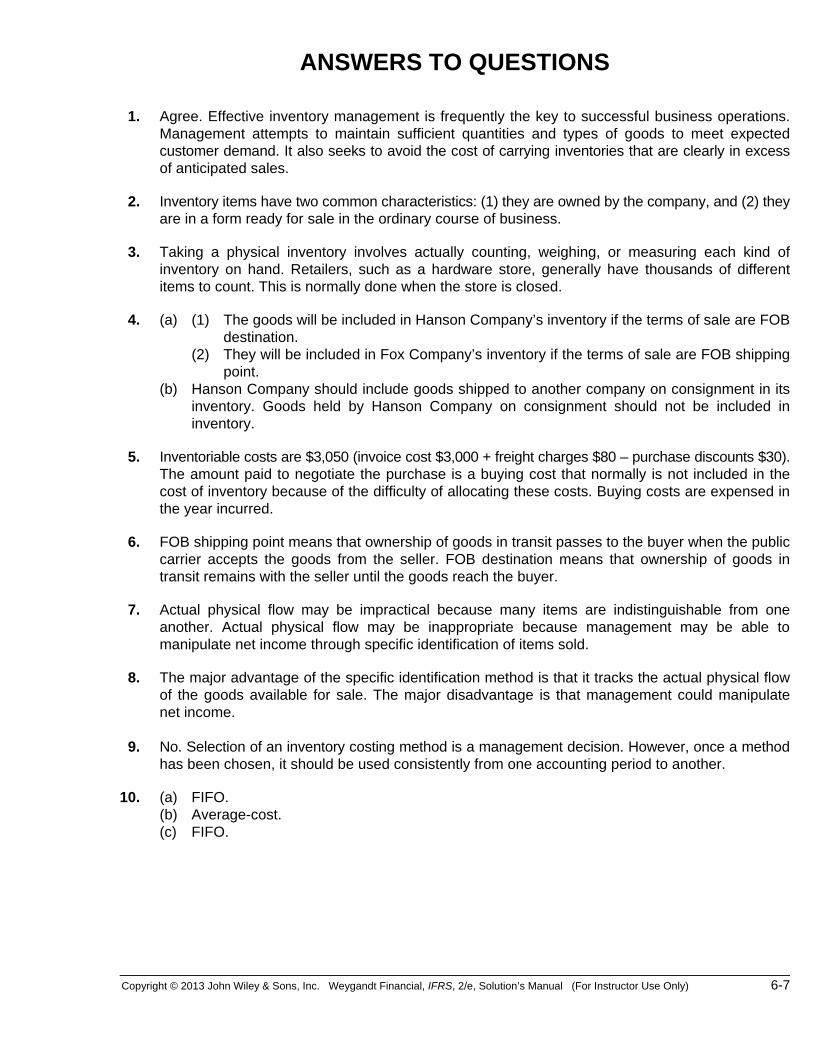
ANSWERS TO QUESTIONS 1. Agree. Effective inventory management is frequently the key to successful business operations.
Management attempts to maintain sufficient quantities and types of goods to meet expected customer demand. It also seeks to avoid the cost of carrying inventories that are clearly in excess of anticipated sales.
2. Inventory items have two common characteristics: (1) they are owned by the company, and (2) they
are in a form ready for sale in the ordinary course of business. 3. Taking a physical inventory involves actually counting, weighing, or measuring each kind of
inventory on hand. Retailers, such as a hardware store, generally have thousands of different items to count. This is normally done when the store is closed.
4. (a) (1) The goods will be included in Hanson Company’s inventory if the terms of sale are FOB
destination. (2) They will be included in Fox Company’s inventory if the terms of sale are FOB shipping
point. (b) Hanson Company should include goods shipped to another company on consignment in its
inventory. Goods held by Hanson Company on consignment should not be included in inventory.
5. Inventoriable costs are $3,050 (invoice cost $3,000 + freight charges $80 – purchase discounts $30).
The amount paid to negotiate the purchase is a buying cost that normally is not included in the cost of inventory because of the difficulty of allocating these costs. Buying costs are expensed in the year incurred.
6. FOB shipping point means that ownership of goods in transit passes to the buyer when the public
carrier accepts the goods from the seller. FOB destination means that ownership of goods in transit remains with the seller until the goods reach the buyer.
7. Actual physical flow may be impractical because many items are indistinguishable from one
another. Actual physical flow may be inappropriate because management may be able to manipulate net income through specific identification of items sold.
8. The major advantage of the specific identification method is that it tracks the actual physical flow
of the goods available for sale. The major disadvantage is that management could manipulate net income.
9. No. Selection of an inventory costing method is a management decision. However, once a method
has been chosen, it should be used consistently from one accounting period to another. 10. (a) FIFO. (b) Average-cost. (c) FIFO.

6-8 Copyright © 2013 John Wiley & Sons, Inc. Weygandt Financial, IFRS, 2/e, Solution’s Manual (For Instructor Use Only)
Questions Chapter 6 (Continued) 11. Steve should know the following:
(a) A departure from the cost basis of accounting for inventories is justified when the value of the goods is lower than its cost. The writedown to net realizable value should be recognized in the period in which the price decline occurs.
(b) Net realizable value (NRV) means the net amount that a company expects to realize from the sale, not the selling price. NRV is estimated selling price less estimated costs to complete and to make a sale.
12. Steering Music Center should report the DVD players at $90 each for a total of $450. $90
is the net realizable value under the lower-of-cost-or-net realizable value basis of accounting for inventories. A decline in net realizable value usually leads to a decline in the selling price of the item. Valuation at LCNRV is an example of the accounting concept of prudence.
13. Maggie Stores should report the toasters at $28 each for a total of $560. The $28 is the lower of cost
or net realizable value. 14. (a) Cohen Company’s 2013 net income will be understated €7,600; (b) 2014 net income will be
overstated €7,600; and (c) the combined net income for the two years will be correct. 15. Raglan Company should disclose: (1) the major inventory classifications, (2) the basis of
accounting (cost or lower of cost or net realizable value), and (3) the costing method (FIFO or average cost).
16. An inventory turnover that is too high may indicate that the company is losing sales opportunities
because of inventory shortages. Inventory outages may also cause customer ill will and result in lost future sales.
*17. In a periodic system, the average is a weighted average based on total goods available for sale for the
period. In a perpetual system, the average is a moving average of goods available for sale after each purchase.
*18. Inventories must be estimated when: (1) management wants monthly or quarterly financial
statements but a physical inventory is only taken annually and (2) a fire or other type of casualty makes it impossible to take a physical inventory.
*19. In the gross profit method, the average is the gross profit rate, which is gross profit divided by net
sales. The rate is often based on last year’s actual rate. The gross profit rate is applied to net sales in using the gross profit method.
In the retail inventory method, the average is the cost-to-retail ratio, which is the goods available
for sale at cost divided by the goods available for sale at retail. The ratio is based on current year data and is applied to the ending inventory at retail.

Copyright © 2013 John Wiley & Sons, Inc. Weygandt Financial, IFRS, 2/e, Solution’s Manual (For Instructor Use Only) 6-9
Questions Chapter 6 (Continued) *20. The estimated cost of the ending inventory is $60,000:
Net sales ................................................................................................................... $400,000 Less: Gross profit ($400,000 X 40%) ....................................................................... 160,000 Estimated cost of goods sold .................................................................................... $240,000
Cost of goods available for sale ................................................................................ $300,000 Less: Cost of goods sold .......................................................................................... 240,000 Estimated cost of ending inventory ........................................................................... $ 60,000 *21. The estimated cost of the ending inventory is €21,000: Ending inventory at retail: €30,000 = (€120,000 – €90,000)
Cost-to-retail ratio: 70% = 84, 000120, 000
⎛ ⎞⎜ ⎟⎝ ⎠
€€
Ending inventory at cost: €21,000 = (€30,000 X 70%) *22. Barto Company is using the FIFO method of inventory costing, and Phelan Company is using the
LIFO method. Under FIFO, the latest goods purchased remain in inventory. Thus, the inventory on the statement of financial position should be close to current costs. The reverse is true of the LIFO method. Barto Company will have the higher gross profit because cost of goods sold will include a higher proportion of goods purchased at earlier (lower) costs.
*23. Disagree. The results under the FIFO method are the same but the results under the LIFO
method are different. The reason is that the pool of inventoriable costs (cost of goods available for sale) is not the same. Under a periodic system, the pool of costs is the goods available for sale for the entire period, whereas under a perpetual system, the pool is the goods available for sale up to the date of sale.
*24. During times of rising prices, using the LIFO method for costing inventories rather than FIFO or
average-cost will result in lower income taxes. Since LIFO uses the most recent, higher, costs to calculate cost of goods sold, taxable income is lower, and income taxes are also lower.

6-10 Copyright © 2013 John Wiley & Sons, Inc. Weygandt Financial, IFRS, 2/e, Solution’s Manual (For Instructor Use Only)
SOLUTIONS TO BRIEF EXERCISES
BRIEF EXERCISE 6-1 (a) Ownership of the goods belongs to Dayne. Thus, these goods should
be included in Dayne’s inventory. (b) The goods in transit should not be included in the inventory count
because ownership by Dayne does not occur until the goods reach Dayne (the buyer).
(c) The goods being held belong to the customer. They should not be
included in Dayne’s inventory. (d) Ownership of these goods rests with the other company. Thus, these
goods should not be included in Dayne’s inventory. BRIEF EXERCISE 6-2 The items that should be included in goods available for sale are: (a) Freight-In (b) Purchase Returns and Allowances (c) Purchases (e) Purchase Discounts BRIEF EXERCISE 6-3 (a) The ending inventory under FIFO consists of 200 units at $8 + 250 units
at $7 for a total allocation of $3,350 or ($1,600 + $1,750). (b) Average unit cost is $6.89 computed as follows: 300 X $6 = $1,800 400 X $7 = 2,800 200 X $8 = 1,600 900 $6,200 $6,200 ÷ 900 = $6.89 (rounded). The cost of the ending inventory is $3,100.50 or (450 X $6.89).

Copyright © 2013 John Wiley & Sons, Inc. Weygandt Financial, IFRS, 2/e, Solution’s Manual (For Instructor Use Only) 6-11
BRIEF EXERCISE 6-4 (a) FIFO would result in the higher net income. (b) FIFO would result in the higher ending inventory. (c) Average-cost would result in the lower income tax expense (because
it would result in the lower taxable income). (d) Average-cost would result in the more stable income over a number
of years because it averages out any big changes in the cost of inventory. BRIEF EXERCISE 6-5 Inventory Categories
Cost
NRV
Lower -of-cost -or-NRV
Cameras £12,000 £12,100 £12,000Camcorders 9,500 9,200 9,200DVD players 14,000 12,800 12,800 Total valuation £34,000 BRIEF EXERCISE 6-6 The understatement of ending inventory caused cost of goods sold to be overstated $5,000 and net income to be understated $5,000. The correct net income for 2014 is $95,000 or ($90,000 + $5,000). Total assets in the statement of financial position will be understated by the amount that ending inventory is understated, $5,000. BRIEF EXERCISE 6-7
Inventory turnover: ( )$300,000
$60,000 + $40,000 ÷ 2 = $300,000
$50,000 = 6.0
Days in inventory: 3656.0
= 60.8 days

6-12 Copyright © 2013 John Wiley & Sons, Inc. Weygandt Financial, IFRS, 2/e, Solution’s Manual (For Instructor Use Only)
*BRIEF EXERCISE 6-8 (a) FIFO Method Product E2-D2
Date
Purchases Cost of
Goods Sold
Balance May 7 (50 @ $11) $550 (50 @ $11) $550 June 1 (30 @ $11) $330 (20 @ $11) $220 July 28 (30 @ $13) $390 (20 @ $11) } $610 (30 @ $13) Aug. 27 (20 @ $11) } $415 (15 @ $13) (15 @ $13) $195
(b) Average-Cost Product E2-D2
Date
Purchases Cost of
Goods Sold
Balance May 7 (50 @ $11) $550 (50 @ $11) $550 June 1 (30 @ $11) $330 (20 @ $11) $220 July 28 (30 @ $13) $390 (50 @ $12.20)* $610 Aug. 27 (35 @ $12.20) $427 (15 @ $12.20) $183
*($220 + $390) ÷ 50
*BRIEF EXERCISE 6-9 (1) Net sales ............................................................................. ¥330,000 Less: Estimated gross profit (40% X ¥330,000) .............. 132,000 Estimated cost of goods sold ........................................... ¥198,000 (2) Cost of goods available for sale ....................................... ¥230,000 Less: Estimated cost of goods sold ................................ 198,000 Estimated cost of ending inventory ................................. ¥ 32,000
Copyright © 2013 John Wiley & Sons, Inc. Weygandt Financial, IFRS, 2/e, Solution’s Manual (For Instructor Use Only) 6-13
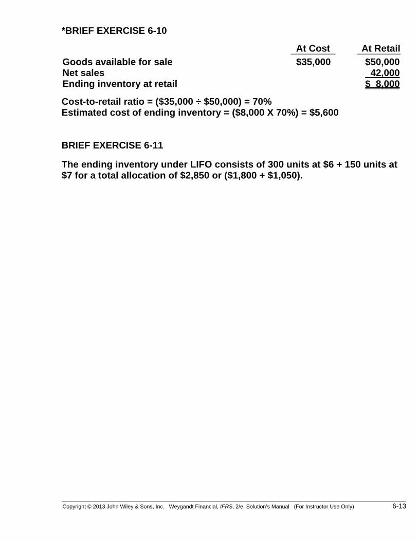
*BRIEF EXERCISE 6-10 At Cost At Retail
Goods available for sale $35,000 $50,000Net sales 42,000Ending inventory at retail $ 8,000 Cost-to-retail ratio = ($35,000 ÷ $50,000) = 70% Estimated cost of ending inventory = ($8,000 X 70%) = $5,600
BRIEF EXERCISE 6-11 The ending inventory under LIFO consists of 300 units at $6 + 150 units at $7 for a total allocation of $2,850 or ($1,800 + $1,050).

6-14 Copyright © 2013 John Wiley & Sons, Inc. Weygandt Financial, IFRS, 2/e, Solution’s Manual (For Instructor Use Only)
SOLUTIONS FOR DO IT! REVIEW EXERCISES
DO IT! 6-1 Inventory per physical count .................................................... R$300,000 Inventory out on consignment ................................................. 21,000 Inventory purchased, in transit at year-end ............................ 20,000 Inventory sold, in transit at year-end ....................................... –0– Correct December 31 inventory................................................ R$341,000 DO IT! 6-2 Cost of goods available for sale = (3,000 X $5) + (8,000 X $7) = $71,000 Ending inventory = 3,000 + 8,000 – 9,400 = 1,600 units (a) FIFO: $71,000 – (1,600 X $7) = $59,800 (b) Average-cost: $71,000/11,000 = $6.455 per unit 9,400 X $6.455 = $60,677 DO IT! 6-3 (a) The lower value for each inventory type is: Small $64,000, Medium
$260,000, and Large $149,000. The total inventory value is the sum of these figures, $473,000.
(b) 2013 2014 Ending inventory $28,000 understated No effect Cost of goods sold $28,000 overstated $28,000 understated Equity $28,000 understated No effect

Copyright © 2013 John Wiley & Sons, Inc. Weygandt Financial, IFRS, 2/e, Solution’s Manual (For Instructor Use Only) 6-15
DO IT! 6-4
2013 2014
Inventory turnover ratio CHF1,200,000 = 6 CHF1,425,000 = 8.9(CHF180,000 + CHF220,000)/2
(CHF220,000 + CHF100,000)/2
Days in inventory 365 ÷ 6 = 60.8 days 365 ÷ 8.9 = 41.0 days The company experienced a very significant decline in its ending inventory as a result of the just-in-time inventory. This decline improved its inventory turnover ratio and its days in inventory. It appears that this change is a win-win situation for Lousanne Company.

6-16 Copyright © 2013 John Wiley & Sons, Inc. Weygandt Financial, IFRS, 2/e, Solution’s Manual (For Instructor Use Only)
SOLUTIONS TO EXERCISES EXERCISE 6-1 Ending inventory—physical count ................................................. $297,000 1. No effect: Title passes to purchaser upon shipment when terms are FOB shipping point ................................... 0 2. No effect: Title does not transfer to Alou until goods are received ............................................................... 0 3. Add to inventory: Title passed to Alou when goods were shipped ......................................................................... 19,000 4. Add to inventory: Title remains with Alou until purchaser receives goods ................................................... 35,000 5. No effect: Title passes to purchaser upon shipment when terms are FOB shipping point .................................. 0 Correct inventory ............................................................................. $351,000 EXERCISE 6-2 Ending inventory—as reported ...................................................... £740,000
1. Subtract from inventory: The goods belong to Superior Corporation. Platinum is merely holding them as a consignee ............................................................ (250,000)
2. No effect: Title does not pass to Platinum until goods are received (Jan. 3) ................................................. 0
3. Subtract from inventory: Office supplies should be carried in a separate account. They are not considered inventory held for resale.................................. (17,000)
4. Add to inventory: The goods belong to Platinum until they are shipped (Jan. 1) ............................................. 33,000
5. Add to inventory: District Sales ordered goods with a cost of £8,000. Platinum should record the corresponding sales revenue of £10,000. Platinum decision to ship extra “unordered” goods does not constitute a sale. The manager’s statement that District could ship the goods back indicates that Platinum knows this over-shipment is not a legitimate sale. The manager acted unethically in an attempt to improve Platinum reported income by over-shipping ..................................... 52,000

Copyright © 2013 John Wiley & Sons, Inc. Weygandt Financial, IFRS, 2/e, Solution’s Manual (For Instructor Use Only) 6-17
EXERCISE 6-2 (Continued) 6. Subtract from inventory: IFRS require that inventory
be valued at the lower of cost or net realizable value. Obsolete parts should be adjusted from cost to zero if they have no other use . ..................................................... (48,000)
Correct inventory.............................................................................. £510,000 EXERCISE 6-3 (a) FIFO Cost of Goods Sold (#1012) $100 + (#1045) $90 = $190 (b) It could choose to sell specific units purchased at specific costs if it
wished to impact earnings selectively. If it wished to minimize earnings it would choose to sell the units purchased at higher costs—in which case the Cost of Goods Sold would be $190. If it wished to maximize earnings it would choose to sell the units purchased at lower costs—in which case the cost of goods sold would be $174.
(c) I recommend they use the FIFO method because it produces a more
appropriate Statement of Financial Position valuation and reduces the opportunity to manipulate earnings.
(The answer may vary depending on the method the student chooses.) EXERCISE 6-4 (a) FIFO
Beginning inventory (23 X HK$970) .............. HK$ 22,310 Purchases Sept. 12 (45 X HK$1,020) ......................... HK$45,900 Sept. 19 (20 X HK$1,040) ......................... 20,800 Sept. 26 (44 X HK$1,050) ......................... 46,200 112,900 Cost of goods available for sale ................... 135,210 Less: Ending inventory (11 X HK$1,050) ..... 11,550 Cost of goods sold ......................................... HK$123,660

6-18 Copyright © 2013 John Wiley & Sons, Inc. Weygandt Financial, IFRS, 2/e, Solution’s Manual (For Instructor Use Only)
EXERCISE 6-4 (Continued)
Proof Date Units Unit Cost Total Cost 9/1 23 HK$ 970 HK$ 22,310 9/12 45 1,020 45,900 9/19 20 1,040 20,800 9/26 33 1,050 34,650
121 HK$123,660
Average-Cost Cost of goods available for sale ......................................... HK$135,210 Less: Ending inventory (11 X HK$1,024.32*) .................... 11,268 Cost of goods sold .............................................................. HK$123,942 *Average unit cost is HK$1024.32 computed as follows:
HK$135,210 (Cost of goods availablefor sale) =HK$1,024.32 (rounded)
132 units (Total units available for sale)
Proof 121 units X HK$1,024.32 = HK$123,943 (HK$1 difference due
to rounding) (b)
FIFO HK$11,550 (ending inventory) + HK$123,660 (COGS) = HK$135,210 } Cost of goods available for sale
Average-cost HK$11,268 (ending inventory) + HK$123,942 (COGS) = HK$135,210
Under both methods, the sum of the ending inventory and cost of goods sold equals the same amount, HK$135,210, which is the cost of goods available for sale. EXERCISE 6-5
FIFO Beginning inventory (30 X $9) ............................................... $270 Purchases May 15 (25 X $11) ............................................................ $275 May 24 (35 X $12) ............................................................ 420 695 Cost of goods available for sale ............................................ 965 Less: Ending inventory (22 X $12) ....................................... 264 Cost of goods sold ................................................................. $701
Copyright © 2013 John Wiley & Sons, Inc. Weygandt Financial, IFRS, 2/e, Solution’s Manual (For Instructor Use Only) 6-19
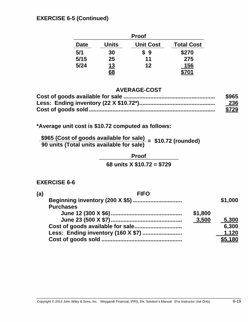
EXERCISE 6-5 (Continued)
Proof Date Units Unit Cost Total Cost5/1 30 $ 9 $270 5/15 25 11 275 5/24 13 12 156
68 $701
AVERAGE-COST Cost of goods available for sale .......................................................... $965 Less: Ending inventory (22 X $10.72*) ................................................ 236 Cost of goods sold ................................................................................ $729 *Average unit cost is $10.72 computed as follows:
$965 (Cost of goods available for sale) = $10.72 (rounded) 90 units (Total units available for sale)
Proof68 units X $10.72 = $729
EXERCISE 6-6 (a) FIFO Beginning inventory (200 X $5) ............................... $1,000 Purchases June 12 (300 X $6) ............................................. $1,800 June 23 (500 X $7) ............................................. 3,500 5,300 Cost of goods available for sale .............................. 6,300 Less: Ending inventory (160 X $7) ......................... 1,120 Cost of goods sold ................................................... $5,180

6-20 Copyright © 2013 John Wiley & Sons, Inc. Weygandt Financial, IFRS, 2/e, Solution’s Manual (For Instructor Use Only)
EXERCISE 6-6 (Continued) AVERAGE-COST Cost of goods available for sale ............................. $6,300 Less: Ending inventory (160 X $6.30*) .................. 1,008 Cost of goods sold ................................................... $5,292 *Average unit cost is:
$6,300 (Cost of goods available for sale) = $6.30 1,000 units (Total units available for sale) (b) The FIFO method will produce the higher ending inventory because
costs have been rising. Under this method, the earliest costs are assigned to cost of goods sold and the latest costs remain in ending inventory. For Eastland Company, the ending inventory under FIFO is $1,120 or (160 X $7) compared to $1,008 or (160 X $6.30) under average-cost.
(c) The average-cost method will produce the higher cost of goods sold
for Eastland Company. The cost of goods sold is $5,292 or [$6,300 –$1,008] compared to $5,180 or ($6,300 – $1,120) under FIFO.
EXERCISE 6-7 (a) (1) FIFO Beginning inventory .......................................... $10,000 Purchases ........................................................... 26,000 Cost of goods available for sale ....................... 36,000 Less: ending inventory (75 X $130*) ................ 9,750 Cost of goods sold ............................................. $26,250 *$26,000 ÷ 200 (2) AVERAGE-COST Beginning inventory .......................................... $10,000 Purchases ........................................................... 26,000 Cost of goods available for sale ....................... 36,000 Less: ending inventory (75 X $120*) ................ 9,000 Cost of goods sold ............................................. $27,000 *[($10,000 + $26,000) ÷ (100 + 200)]

Copyright © 2013 John Wiley & Sons, Inc. Weygandt Financial, IFRS, 2/e, Solution’s Manual (For Instructor Use Only) 6-21
EXERCISE 6-7 (Continued) (b) The use of FIFO would result in the higher net income since the earlier
lower costs are matched with revenues. (c) The use of FIFO would result in inventories approximating current cost in
the statement of financial position, since the more recent units are assumed to be on hand.
(d) The use of average-cost would result in Givens paying lower taxes in the first year since taxable income will be lower.
EXERCISE 6-8
Cost
NRV
Lower-of-Cost -or-NRV
Cameras Minolta W1,360,000 W1,248,000 W1,248,000 Canon 900,000 912,000 900,000Total 2,260,000 2,160,000 Light meters Vivitar 1,500,000 1,380,000 1,380,000 Kodak 1,610,000 1,890,000 1,610,000Total 3,110,000 3,270,000 Total inventory W5,370,000 W5,430,000 W5,138,000 EXERCISE 6-9
Cost
NRV
Lower -of-Cost- or-NRV
Cameras $ 6,800 $ 7,000 $ 6,800 DVD players 11,250 10,350 10,350 iPods 10,000 9,750 9,750 Total inventory $28,050 $27,100 $26,900 EXERCISE 6-10 2013 2014 Beginning inventory............................................. € 20,000 € 28,000 Cost of goods purchased .................................... 150,000 175,000 Cost of goods available for sale ......................... 170,000 203,000 Corrected ending inventory ................................ 28,000a 41,000b Cost of goods sold ............................................... €142,000 €162,000 a€30,000 – €2,000 = €28,000. b€35,000 + €6,000 = €41,000.
6-22 Copyright © 2013 John Wiley & Sons, Inc. Weygandt Financial, IFRS, 2/e, Solution’s Manual (For Instructor Use Only)
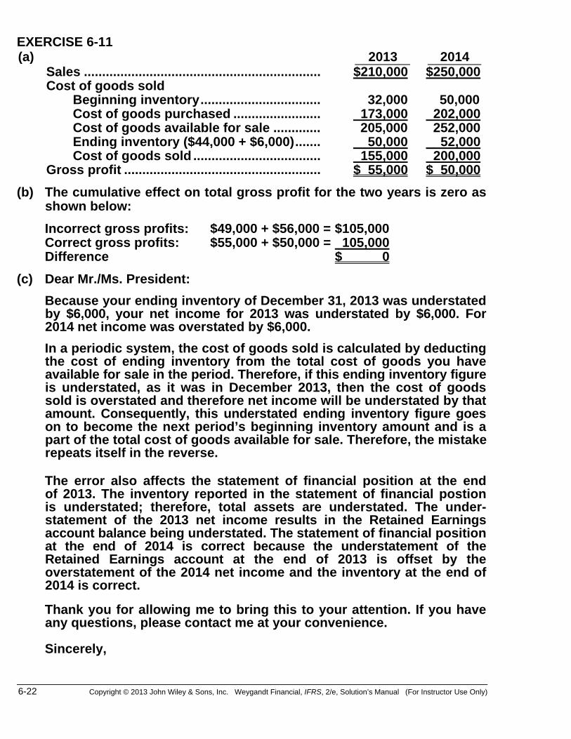
EXERCISE 6-11 (a) 2013 2014
Sales ................................................................. $210,000 $250,000 Cost of goods sold Beginning inventory ................................. 32,000 50,000 Cost of goods purchased ........................ 173,000 202,000 Cost of goods available for sale ............. 205,000 252,000 Ending inventory ($44,000 + $6,000) ....... 50,000 52,000 Cost of goods sold ................................... 155,000 200,000 Gross profit ...................................................... $ 55,000 $ 50,000
(b) The cumulative effect on total gross profit for the two years is zero as
shown below: Incorrect gross profits: $49,000 + $56,000 = $105,000 Correct gross profits: $55,000 + $50,000 = 105,000 Difference $ 0 (c) Dear Mr./Ms. President: Because your ending inventory of December 31, 2013 was understated
by $6,000, your net income for 2013 was understated by $6,000. For 2014 net income was overstated by $6,000.
In a periodic system, the cost of goods sold is calculated by deducting
the cost of ending inventory from the total cost of goods you have available for sale in the period. Therefore, if this ending inventory figure is understated, as it was in December 2013, then the cost of goods sold is overstated and therefore net income will be understated by that amount. Consequently, this understated ending inventory figure goes on to become the next period’s beginning inventory amount and is a part of the total cost of goods available for sale. Therefore, the mistake repeats itself in the reverse.
The error also affects the statement of financial position at the end
of 2013. The inventory reported in the statement of financial postion is understated; therefore, total assets are understated. The under-statement of the 2013 net income results in the Retained Earnings account balance being understated. The statement of financial position at the end of 2014 is correct because the understatement of the Retained Earnings account at the end of 2013 is offset by the overstatement of the 2014 net income and the inventory at the end of 2014 is correct.
Thank you for allowing me to bring this to your attention. If you have
any questions, please contact me at your convenience. Sincerely,

Copyright © 2013 John Wiley & Sons, Inc. Weygandt Financial, IFRS, 2/e, Solution’s Manual (For Instructor Use Only) 6-23
EXERCISE 6-12 2012 2013 2014 Inventory turnover
$900,000 $1,120,000 $1,300,000 ($100,000 + $330,000) ÷ 2 ($330,000 + $400,000) ÷ 2 ($400,000 + $480,000) ÷ 2
$900,000 = 4.19 $1,120,000 = 3.07 $1,300,000 = 2.95 $215,000 $365,000 $440,000 Days in inventory
365 = 87.1 days 365 = 118.9 days 365 = 123.7 days 4.19 3.07 2.95 Gross profit rate
$1,200,000 – $900,000 = .25 $1,600,000 – $1,120,000 = .30
$1,900,000 – $1,300,000 = .32$1,200,000 $1,600,000 $1,900,000 The inventory turnover ratio decreased by approximately 30% from 2012 to 2014 while the days in inventory increased by almost 42% over the same time period. Both of these changes would be considered negative since it’s better to have a higher inventory turnover with a correspondingly lower days in inventory. However, Sepia Photo’s gross profit rate increased by 28% from 2012 to 2014, which is a positive sign. EXERCISE 6-13 (a) Gouda Company Edam Company
Inventory Turnover €192,000 €292,000 (€47,000 + €55,000)/2
= 3.76 (€71,000 + €69,000)/2
= 4.17
Days in Inventory 365/3.76 = 97 days 365/4.17 = 88 days (b) Edam Company is moving its inventory quicker, since its inventory
turnover is higher, and its days in inventory is lower.

6-24 Copyright © 2013 John Wiley & Sons, Inc. Weygandt Financial, IFRS, 2/e, Solution’s Manual (For Instructor Use Only)
*EXERCISE 6-14 (1) FIFO Date Purchases Cost of Goods Sold Balance Jan. 1 (3 @ $600) $1,800 8 (2 @ $600) $1,200 (1 @ $600) 600 10 (6 @ $648) $3,888 (1 @ $600) 4,488 (6 @ $648) 15 (1 @ $600) (3 @ $648) $2,544 (3 @ $648) 1,944 (2) MOVING-AVERAGE COST Date Purchases Cost of Goods Sold Balance Jan. 1 (3 @ $600) $1,800 8 (2 @ $600) $1,200 (1 @ $600) 600 10 (6 @ $648) $3,888 (7 @ $641.14)* 4,488 15 (4 @ $641.14) $2,565 (3 @ $641.14) 1,923 *Average-cost = ($600 + $3,888) ÷ 7 = $641.14 (rounded) *EXERCISE 6-15
The cost of goods available for sale is:
June 1 Inventory 200 @ $5 $1,000 June 12 Purchase 300 @ $6 1,800 June 23 Purchase 500 @ $7 3,500 Total cost of goods available for sale $6,300

Copyright © 2013 John Wiley & Sons, Inc. Weygandt Financial, IFRS, 2/e, Solution’s Manual (For Instructor Use Only) 6-25
*EXERCISE 6-15 (Continued)
(1) FIFODate Purchases Cost of Goods Sold Balance June 1 (200 @ $5) $1,000June 12 (300 @ $6) $1,800 (200 @ $5) } $2,800 (300 @ $6)June 15 (200 @ $5) $1,000 (200 @ $6) 1,200 (100 @ $6) $ 600 (100 @ $6) } $4,100June 23 (500 @ $7) $3,500 (500 @ $7) June 27 (100 @ $6) 600 (340 @ $7) 2,380 (160 @ $7) $1,120 $5,180 Ending inventory: $1,120. Cost of goods sold: $6,300 – $1,120 = $5,180.
(2) Moving-Average Cost Date Purchases Cost of Goods Sold Balance June 1 (200 @ $5) $1,000June 12 (300 @ $6) $1,800 (500 @ $5.60) $2,800June 15 (400 @ $5.60) $2,240 (100 @ $5.60) $ 560June 23 (500 @ $7) $3,500 (600 @ $6.767) $4,060June 27 (440 @ $6.767) $2,977 (160 @ $6.767) $1,083 $5,217 Ending inventory: $1,083. Cost of goods sold: $6,300 – $1,083 = $5,217. (b) FIFO gives the same ending inventory and cost of goods sold values
under both the periodic and perpetual inventory system. Moving average gives different ending inventory and cost of goods sold values under the periodic and perpetual inventory systems, due to the average calculation being based on different pools of costs.
(c) The simple average would be [($5 + $6 + $7) ÷ 3)] or $6. However, the
moving-average cost method uses a weighted-average unit cost that changes each time a purchase is made rather than a simple average.

6-26 Copyright © 2013 John Wiley & Sons, Inc. Weygandt Financial, IFRS, 2/e, Solution’s Manual (For Instructor Use Only)
*EXERCISE 6-16 (a)
FIFO
Date
Purchases
Cost of
Goods Sold
Balance
9/1 (23 @ HK$ 970) HK$22,310
9/5 (12 @ HK$ 970) HK$11,640 (11 @ HK$ 970) HK$10,670 9/12 (45 @ HK$1,020) HK$45,900 (11 @ HK$ 970)
HK$56,570 (45 @ HK$1,020) 9/16 (11 @ HK$ 970) (39 @ HK$1,020) HK$50,450 ( 6 @ HK$1,020) HK$ 6,120 9/19 (20 @ HK$1,040) HK$20,800 ( 6 @ HK$1,020)
HK$26,920 (20 @ HK$1,040) 9/26 (44 @ HK$1,050) HK$46,200 ( 6 @ HK$1,020) (20 @ HK$1,040) HK$73,120 (44 @ HK$1,050) 9/29 ( 6 @ HK$1,020) (20 @ HK$1,040) (33 @ HK$1,050) HK$61,570 (11 @ HK$1,050) HK$11,550
Moving-Average Cost
Date
Purchases
Cost of
Goods Sold
Balance
9/1 (23 @ HK$970) HK$22,310
9/5 (12 @ HK$970) HK$11,640 (11 @ HK$970) HK$10,670 9/12 (45 @ HK$1,020) HK$45,900 (56 @ HK$1,010.18)a HK$56,570 9/16 (50 @ HK$1,010.18) HK$50,509* * ( 6 @ HK$1,010.18) HK$ 6,061 9/19 (20 @ HK$1040) HK$20,800 (26 @ HK$1,033.12)b HK$26,861 9/26 (44 @ HK$1050) HK$46,200 (70 @ HK$1,043.73)c HK$73,061 9/29 (59 @ HK$1,043.73) HK$61,580* (11 @ HK$1,043.73) HK$11,481
*Rounded a HK$56,570 ÷ 56 = HK$1,010.18 b HK$26,861 ÷ 26 = HK$1,033.12 c HK$73,061 ÷ 70 = HK$1,043.73

Copyright © 2013 John Wiley & Sons, Inc. Weygandt Financial, IFRS, 2/e, Solution’s Manual (For Instructor Use Only) 6-27
*EXERCISE 6-16 (Continued) (b)
Periodic . PerpetualEnding Inventory FIFO HK$11,550 HK$11,550Ending Inventory Average HK$11,268 HK$11,481
(c) FIFO yields the same ending inventory value under both the periodic
and perpetual inventory system. Average cost yields different ending inventory values when using the
periodic versus perpetual inventory system. *EXERCISE 6-17 (a) Sales ....................................................................... Rs7,500,000 Cost of goods sold Inventory, November 1 Rs1,000,000 Cost of goods purchased ............................ 5,000,000 Cost of goods available for sale ................. 6,000,000 Inventory, December 31 .............................. 1,200,000 Cost of goods sold ............................. 4,800,000 Gross profit ............................................................ Rs2,700,000 Gross profit rate Rs2,700,000/Rs7,500,000 = 36% (b) Sales Rs10,000,000 Less: Estimated gross profit (36% X Rs10,000,000) 3,600,000 Estimated cost of goods sold Rs 6,400,000 Beginning inventory ........................................................... Rs 1,200,000 Cost of goods purchased .................................................. 6,100,000 Cost of goods available for sale ........................................ 7,300,000 Less: Estimated cost of goods sold ................................ 6,400,000 Estimated cost of ending inventory .................................. Rs 900,000
6-28 Copyright © 2013 John Wiley & Sons, Inc. Weygandt Financial, IFRS, 2/e, Solution’s Manual (For Instructor Use Only)
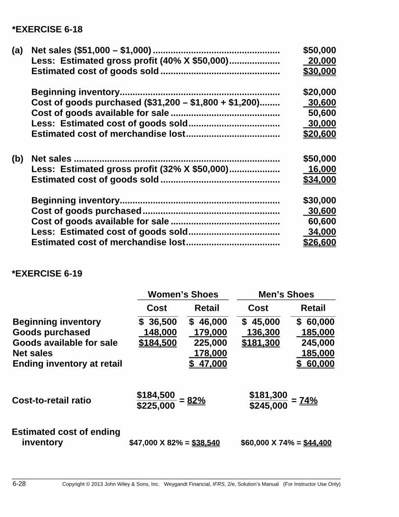
*EXERCISE 6-18 (a) Net sales ($51,000 – $1,000) .................................................. $50,000 Less: Estimated gross profit (40% X $50,000) .................... 20,000 Estimated cost of goods sold ............................................... $30,000 Beginning inventory............................................................... $20,000 Cost of goods purchased ($31,200 – $1,800 + $1,200) ........ 30,600 Cost of goods available for sale ........................................... 50,600 Less: Estimated cost of goods sold .................................... 30,000 Estimated cost of merchandise lost ..................................... $20,600 (b) Net sales ................................................................................. $50,000 Less: Estimated gross profit (32% X $50,000) .................... 16,000 Estimated cost of goods sold ............................................... $34,000 Beginning inventory............................................................... $30,000 Cost of goods purchased ...................................................... 30,600 Cost of goods available for sale ........................................... 60,600 Less: Estimated cost of goods sold .................................... 34,000 Estimated cost of merchandise lost ..................................... $26,600 *EXERCISE 6-19 Women’s Shoes Men’s Shoes
Cost Retail Cost RetailBeginning inventory $ 36,500 $ 46,000 $ 45,000 $ 60,000Goods purchased 148,000 179,000 136,300 185,000Goods available for sale $184,500 225,000 $181,300 245,000Net sales 178,000 185,000Ending inventory at retail $ 47,000 $ 60,000
Cost-to-retail ratio $184,500 = 82% $181,300 = 74% $225,000 $245,000
Estimated cost of ending inventory $47,000 X 82% = $38,540 $60,000 X 74% = $44,400

Copyright © 2013 John Wiley & Sons, Inc. Weygandt Financial, IFRS, 2/e, Solution’s Manual (For Instructor Use Only) 6-29
*EXERCISE 6-20 LIFO Beginning inventory (200 X $5) ........................ $1,000 Purchases June 12 (300 X $6) ...................................... $1,800 June 23 (500 X $7) ...................................... 3,500 5,300 Cost of goods available for sale ....................... 6,300 Less: Ending inventory (160 X $5) .................. 800 Cost of goods sold ............................................ $5,500
*EXERCISE 6-21 (a) LIFO Beginning inventory ........................................... $10,000 Purchases ........................................................... 26,000 Cost of goods available for sale ........................ 36,000 Less: ending inventory (75 X $100) .................. 7,500 Cost of goods sold ............................................. $28,500 (b) The use of FIFO would result in the higher net income since the earlier
lower costs are matched with revenues. (c) The use of FIFO would result in inventories approximating current cost in
the statement of financial position, since the more recent units are assumed to be on hand.
(d) The use of average-cost would result in Givens paying lower taxes in
the first year since taxable income will be lower.

6-30 Copyright © 2013 John Wiley & Sons, Inc. Weygandt Financial, IFRS, 2/e, Solution’s Manual (For Instructor Use Only)
SOLUTIONS TO PROBLEMS
PROBLEM 6-1A (a) The goods should not be included in inventory as they were shipped
FOB shipping point and shipped February 26. Title to the goods transfers to the customer February 26. Anatolia should have recorded the transaction in the Sales Revenue and Accounts Receivable accounts.
(b) The amount should not be included in inventory as they were shipped
FOB destination and not received until March 2. The seller still owns the inventory. No entry is recorded.
(c) Include $620 in inventory. (d) Include $400 in inventory. (e) $750 should be included in inventory as the goods were shipped FOB
shipping point. (f) The sale will be recorded on March 2. The goods should be included
in inventory at the end of February at their cost of $220. (g) The damaged goods should not be included in inventory. They should
be recorded in a loss account since they are not saleable.

Copyright © 2013 John Wiley & Sons, Inc. Weygandt Financial, IFRS, 2/e, Solution’s Manual (For Instructor Use Only) 6-31
PROBLEM 6-2A
(a) COST OF GOODS AVAILABLE FOR SALE Date Explanation Units Unit Cost Total Cost March 1 Beginning Inventory 1,500 $ 7 $ 10,500 5 Purchase 3,500 8 28,000 13 Purchase 4,000 9 36,000 21 Purchase 2,000 10 20,000 26 Purchase 2,000 11 22,000 Total 13,000 $116,500 (b) FIFO (1) Ending Inventory (2) Cost of Goods Sold
Date
Units Unit
CostTotal Cost
Cost of goods available for sale
$116,500
March 26 2,000 $11 $22,000 Less: Ending inventory 32,000 21 1,000 10 10,000
3,000* $32,000 Cost of goods sold $ 84,500
*13,000 – 10,000 = 3,000
Proof of Cost of Goods Sold Date
Units
Unit Cost
Total Cost
March 1 1,500 $ 7 $10,500 5 3,500 8 28,000 13 4,000 9 36,000 21 1,000 10 10,000
10,000 $84,500

6-32 Copyright © 2013 John Wiley & Sons, Inc. Weygandt Financial, IFRS, 2/e, Solution’s Manual (For Instructor Use Only)
PROBLEM 6-2A (Continued) AVERAGE-COST (1) Ending Inventory (2) Cost of Goods Sold $116,500 ÷ 13,000 = $8.9615 Cost of goods
available for sale
$116,500
Units Unit
Cost
Total CostLess: Ending inventory
26,885
3,000 $8.9615 $26,885 Cost of goods sold $ 89,615 *rounded to nearest dollar
Proof of Cost of Goods Sold 10,000 units X $8.9615 = $89,615
(c) (1) As shown in (b) above, FIFO produces the higher inventory amount,
$32,000. (2) As shown in (b) above, Average-cost produces the higher cost of
goods sold, $89,615.

Copyright © 2013 John Wiley & Sons, Inc. Weygandt Financial, IFRS, 2/e, Solution’s Manual (For Instructor Use Only) 6-33
PROBLEM 6-3A (a) COST OF GOODS AVAILABLE FOR SALE Date Explanation Units Unit Cost Total Cost 1/1 Beginning Inventory 400 £ 8 £ 3,200 2/20 Purchase 300 9 2,700 5/5 Purchase 500 10 5,000 8/12 Purchase 600 11 6,600 12/8 Purchase 200 12 2,400 Total 2,000 £19,900 (b) FIFO (1) Ending Inventory (2) Cost of Goods Sold
Date
Units Unit
CostTotal Cost
Cost of goods available for sale
£19,900
12/8 200 £12 £2,400 Less: Ending inventory 5,7008/12 300 11 3,300
500* £5,700 Cost of goods sold £14,200 *2,000 – 1,500 = 500
Proof of Cost of Goods Sold Date
Units
Unit Cost
Total Cost
1/1 400 £ 8 £ 3,2002/20 300 9 2,7005/5 500 10 5,0008/12 300 11 3,300
1,500 £14,200

6-34 Copyright © 2013 John Wiley & Sons, Inc. Weygandt Financial, IFRS, 2/e, Solution’s Manual (For Instructor Use Only)
PROBLEM 6-3A (Continued) AVERAGE-COST (1) Ending Inventory (2) Cost of Goods Sold £19,900 ÷ 2,000 = £9.95 Cost of goods
available for sale
£19,900
Units Unit
Cost Total
Cost Less: Ending inventory
4,975
500 £9.95 £4,975 Cost of goods sold £14,925
Proof of Cost of Goods Sold 1,500 units X £9.95 = £14,925 (c) (1) Average-cost results in the lower inventory amount for the
statement of financial position, £4,975. (2) FIFO results in the lower cost of goods sold, £14,200.

Copyright © 2013 John Wiley & Sons, Inc. Weygandt Financial, IFRS, 2/e, Solution’s Manual (For Instructor Use Only) 6-35
PROBLEM 6-4A
(a) RED ROBIN CO. Condensed Income Statement For the Year Ended December 31, 2014
FIFO Average-cost
Sales revenue ............................................. $865,000 $865,000 Cost of goods sold Beginning inventory .......................... 22,800 22,800 Cost of goods purchased .................. 578,500 578,500 Cost of goods available for sale ....... 601,300 601,300 Ending inventory ................................ 39,750a 37,575b Cost of goods sold ............................. 561,550 563,725 Gross profit ................................................ 303,450 301,275 Operating expenses .................................. 147,000 147,000 Income before income taxes .................... 156,450 154,275 Income tax expense (32%) ........................ 50,064 49,368 Net income ................................................. $106,386 $104,907 a15,000 X $2.65 = $39,750. b$601,300 ÷ 240,000 units = $2.505.
15,000 x $2.505 = $37,575
(b) (1) The FIFO method produces the more meaningful inventory amount for the statement of financial position because the units are costed at the most recent purchase prices.
(2) The FIFO method is most likely to approximate actual physical flow
because the oldest goods are usually sold first to minimize spoilage and obsolescence.
(3) There will be $696 additional cash available under average-cost
because income taxes are $49,368 under average-cost and $50,064 under FIFO.

6-36 Copyright © 2013 John Wiley & Sons, Inc. Weygandt Financial, IFRS, 2/e, Solution’s Manual (For Instructor Use Only)
PROBLEM 6-5A
Cost of Goods Available for Sale Date Explanation Units Unit Cost Total CostOctober 1 Beginning Inventory 60 €24 €1,440 9 Purchase 120 26 3,120 17 Purchase 70 27 1,890 25 Purchase 80 28 2,240
Total 330 €8,690 Ending Inventory in Units: Sales Revenue Units available for sale 330 Unit Sales (100 + 65 + 120) 285 Date Units Price Total SalesUnits remaining in ending inventory 45 October 11 100 €35 € 3,500 22 65 40 2,600 29 120 40 4,800 285 €10,900 (a) (1) FIFO (i) Ending Inventory (ii) Cost of Goods Sold October 25
45 @ €28 = €1,260 Cost of goods available for sale
€ 8,690
Less: Ending inventory 1,260 Cost of goods sold € 7,430 (iii) Gross Profit (iv) Gross Profit RateSales revenue €10,900 Gross profit € 3,470 = 31.8% Cost of goods sold 7,430 Net sales €10,900 Gross profit € 3,470

Copyright © 2013 John Wiley & Sons, Inc. Weygandt Financial, IFRS, 2/e, Solution’s Manual (For Instructor Use Only) 6-37
PROBLEM 6-5A (Continued)
(2) Average-Cost Weighted-average cost per unit: cost of goods available for sale
units available for sale €8,690 = €26.333 330 (i) Ending Inventory (ii) Cost of Goods Sold
45 @ €26.333 = €1,185*
Cost of goods available for sale €8,690
*rounded to nearest dollar Less: Ending inventory 1,185 Cost of goods sold €7,505 (iii) Gross Profit (iv) Gross Profit RateSales revenue €10,900 Gross profit € 3,395 = 31.1% Cost of goods sold 7,505 Net sales €10,900Gross profit € 3,395 (b) Average-cost produces the lower ending inventory value, gross profit,
and gross profit rate because its cost of goods sold is higher than FIFO.

6-38 Copyright © 2013 John Wiley & Sons, Inc. Weygandt Financial, IFRS, 2/e, Solution’s Manual (For Instructor Use Only)
PROBLEM 6-6A
(a) (1) To maximize gross profit, Greco Diamonds should sell the diamonds
with the lowest cost. Sale Date Cost of Goods Sold Sales Revenue March 5 150 @ $310 $ 46,500 180 @ $600 $108,000 30 @ $350 10,500 400 @ $650 260,000March 25 170 @ $350 59,500
230 @ $380 87,400 580 $203,900 580 $368,000
Gross profit $368,000 – $203,900 = $164,100. (2) To minimize gross profit, Greco Diamonds should sell the diamonds
with the highest cost. Sale Date Cost of Goods Sold Sales Revenue March 5 180 @ $350 $ 63,000 180 @ $600 $108,000March 25 350 @ $380 133,000 400 @ $650 260,000
20 @ $350 7,000 30 @ $310 9,300 580 $212,300 580 $368,000
Gross profit $368,000 – $212,300 = $155,700. (b) FIFO
Cost of goods available for saleMarch 1 Beginning inventory 150 @ $310 $ 46,500
3 Purchase 200 @ $350 70,000 10 Purchase 350 @ $380 133,000
700 $249,500
Goods available for sale 700 Units sold 580 Ending inventory 120 @ $380 $45,600
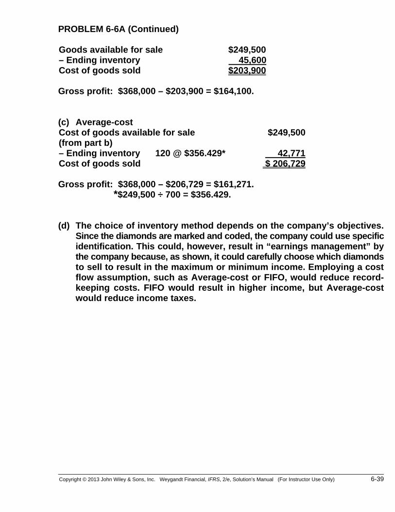
Copyright © 2013 John Wiley & Sons, Inc. Weygandt Financial, IFRS, 2/e, Solution’s Manual (For Instructor Use Only) 6-39
PROBLEM 6-6A (Continued) Goods available for sale $249,500– Ending inventory 45,600Cost of goods sold $203,900 Gross profit: $368,000 – $203,900 = $164,100. (c) Average-cost Cost of goods available for sale $249,500 (from part b) – Ending inventory 120 @ $356.429* 42,771 Cost of goods sold $ 206,729 Gross profit: $368,000 – $206,729 = $161,271.
*$249,500 ÷ 700 = $356.429. (d) The choice of inventory method depends on the company’s objectives.
Since the diamonds are marked and coded, the company could use specific identification. This could, however, result in “earnings management” by the company because, as shown, it could carefully choose which diamonds to sell to result in the maximum or minimum income. Employing a cost flow assumption, such as Average-cost or FIFO, would reduce record-keeping costs. FIFO would result in higher income, but Average-cost would reduce income taxes.

6-40 Copyright © 2013 John Wiley & Sons, Inc. Weygandt Financial, IFRS, 2/e, Solution’s Manual (For Instructor Use Only)
PROBLEM 6-7A (a) TUDOR LTD. Condensed Income Statement For the Year Ended December 31, 2014
FIFO average-cost
Sales revenue ............................................ £665,000 £665,000 Cost of goods sold Beginning inventory ........................... 35,000 35,000 Cost of goods purchased .................. 501,000 501,000 Cost of goods available for sale ........ 536,000 536,000 Ending inventory ................................ 131,000a 123,690b Cost of goods sold ............................. 405,000 412,310 Gross profit ................................................ 260,000 252,690 Operating expenses .................................. 130,000 130,000 Income before income taxes .................... 130,000 122,690 Income tax expense (28%) ....................... 36,400 34,353 Net income ................................................. £ 93,600 £ 88,337 a(20,000 @ £4.45) + (10,000 @ £4.20) = £131,000. b(£536,000 ÷130,000units) = £4.123 per unit; 30,000 @ £4.123 = $123,690
(b) Answers to questions:
(1) The FIFO method produces the most meaningful inventory amount for the statement of financial position because the units are costed at the most recent purchase prices.
(2) The FIFO method is most likely to approximate actual physical
flow because the oldest goods are usually sold first to minimize spoilage and obsolescence.
(3) There will be £2,047 additional cash available under average-cost
because income taxes are £34,353 under average-cost and £36,400 under FIFO.

Copyright © 2013 John Wiley & Sons, Inc. Weygandt Financial, IFRS, 2/e, Solution’s Manual (For Instructor Use Only) 6-41
Answer in business letter form: Dear Tudor Ltd. After preparing the comparative condensed income statements for 2014 under FIFO and average-cost methods, we have found the following: The FIFO method produces the most meaningful inventory amount for the statement of financial position because the units are costed at the most recent purchase prices. This method is most likely to approximate actual physical flow because the oldest goods are usually sold first to minimize spoilage and obsolescence. There will be £2,047 additional cash available under average-cost because income taxes are £34,353 under average-cost and £36,400 under FIFO. Sincerely,

6-42 Copyright © 2013 John Wiley & Sons, Inc. Weygandt Financial, IFRS, 2/e, Solution’s Manual (For Instructor Use Only)
*PROBLEM 6-8A
(a) Sales: Date
January 6 150 units @ $40 $ 6,000 January 9 (return) (10 units @ $40) (400)January 10 50 units @ $45 2,250 January 30 160 units @ $50 8,000
Total sales $15,850 (1) FIFO Date Purchases Cost of Goods Sold Balance January 1 (150 @ $19) $2,850 (150 @ $19) } $4,950 January 2 (100 @ $21) $2,100 (100 @ $21) January 6 (150 @ $19)
$2,850 (100 @ $21) $2,100
January 9 (–10 @ $19) ($ 190) ( 10 @ $19) } $4,090 January 9 ( 75 @ $24) $1,800 (100 @ $21) ( 75 @ $24) ( 10 @ $19) } $3,730 (100 @ $21) January 10 (–15 @ $24) ($ 360) ( 60 @ $24) January 10 ( 10 @ $19) } $1,030 ( 60 @ $21) } $2,700 ( 40 @ $21) ( 60 @ $24) January 23 (100 @ $26) $2,600 ( 60 @ $21) } $5,300 ( 60 @ $24)
(100 @ $26) January 30 ( 60 @ $21)
}
$3,740$7,430
} $1,560 ( 60 @ $24)( 40 @ $26)
( 60 @ $26)
(i) Cost of goods sold = $7,430. (ii) Ending inventory = $1,560. (iii) Gross profit = $15,850 – $7,430 = $8,420.

Copyright © 2013 John Wiley & Sons, Inc. Weygandt Financial, IFRS, 2/e, Solution’s Manual (For Instructor Use Only) 6-43
*PROBLEM 6-8A (Continued) (2) Moving-Average Date Purchases Cost of goods sold Balance January 1 (150 @ $19) $2,850 January 2 (100 @ $21) $2,100 (250 @ $19.80)a $4,950 January 6 (150 @ $19.80) $2,970 (100 @ $19.80) $1,980 January 9 (–10 @ $19.80) ($ 198) (110 @ $19.80) $2,178 January 9 ( 75 @ $24) $1,800 (185 @ $21.503) b $3,978 January 10 (–15 @ $24) ($ 360) (170 @ $21.282) c $3,618 January 10 ( 50 @ $21.282) $1,064 (120 @ $21.282) $2,554 January 23 (100 @ $26) $2,600 (220 @ $23.427) d $5,154 January 30 (160 @ $23.427) $3,748 (60 @ $23.427) $1,406
$7,584 a$4,950 ÷ 250 = $19.80 c$3,618 ÷ 170 = $21.282 b$3,978 ÷ 185 = $21.503 d$5,154 ÷ 220 = $23.427
(i) Cost of goods sold = $7,584. (ii) Ending inventory = $1,406. (iii) Gross profit = $15,850 – $7,584 = $8,266.
(b) FIFO Moving-Average Sales $15,850 $15,850 Cost of goods sold 7,430 7,584 Gross profit $ 8,420 $ 8,266 Ending inventory $ 1,560 $ 1,406
In a period of rising costs, the moving-average cost flow assumption results in the higher cost of goods sold and lower gross profit. FIFO gives the lower cost of goods sold and higher gross profit. On the statement of financial position, FIFO gives the higher ending inventory (representing the most current costs); moving-average gives the lower ending inventory.

6-44 Copyright © 2013 John Wiley & Sons, Inc. Weygandt Financial, IFRS, 2/e, Solution’s Manual (For Instructor Use Only)
*PROBLEM 6-9A
(a) (1) FIFO
Date
Purchases Cost of
Goods Sold
Balance May 1 (7 @ $155) $1,085 (7 @ $155) $1,085 4 (4 @ $155) $620 (3 @ $155) $ 465 8 (8 @ $170) $1,360 (3 @ $155) } $1,825 (8 @ $170) 12 (3 @ $155) } $805 (2 @ $170) (6 @ $170) $1,020 15 (6 @ $185) $1,110 (6 @ $170) } $2,130 (6 @ $185) 20 (3 @ $170) $510 (3 @ $170) } $1,620 (6 @ $185) 25 (3 @ $170) } $880 (2 @ $185) (4 @ $185) $ 740
(2) MOVING-AVERAGE COST
Date
Purchases Cost of
Goods Sold
Balance May 1 (7 @ $155) $1,085 ( 7 @ $155) $1,085 4 (4 @ $155) $620 ( 3 @ $155) $ 465 8 (8 @ $170) $1,360 (11 @ $165.91)* $1,825 12 (5 @ $165.91) $830 ( 6 @ $165.91) $ 995 15 (6 @ $185) $1,110 (12 @ $175.42)** $2,105 20 (3 @ $175.42) $526 ( 9 @ $175.42) $1,579 25 (5 @ $175.42) $877 ( 4 @ $175.42) $ 702
*Average-cost = $1,825 ÷ 11 (rounded)
**$2,105 ÷ 12
(b) (1) The higher ending inventory is $740 under the FIFO method. (2) The lower ending inventory is $702 under the moving-average method.
Copyright © 2013 John Wiley & Sons, Inc. Weygandt Financial, IFRS, 2/e, Solution’s Manual (For Instructor Use Only) 6-45
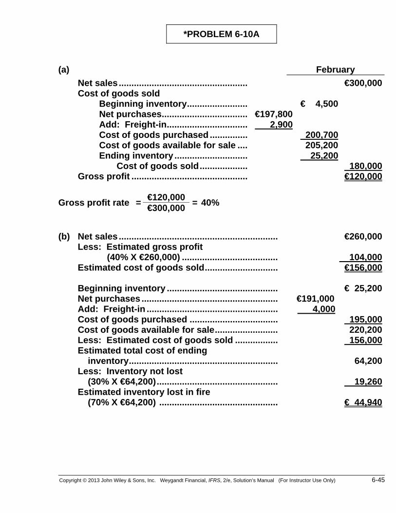
*PROBLEM 6-10A (a) February
Net sales ................................................... €300,000 Cost of goods sold Beginning inventory ........................ € 4,500 Net purchases .................................. €197,800 Add: Freight-in ................................ 2,900 Cost of goods purchased ............... 200,700 Cost of goods available for sale .... 205,200 Ending inventory ............................. 25,200 Cost of goods sold ................... 180,000 Gross profit .............................................. €120,000
Gross profit rate = €120,000 = 40% €300,000
(b) Net sales ............................................................... €260,000 Less: Estimated gross profit (40% X €260,000) ...................................... 104,000 Estimated cost of goods sold ............................. €156,000 Beginning inventory ............................................ € 25,200 Net purchases ...................................................... €191,000 Add: Freight-in .................................................... 4,000 Cost of goods purchased ................................... 195,000 Cost of goods available for sale ......................... 220,200 Less: Estimated cost of goods sold ................. 156,000 Estimated total cost of ending inventory ........................................................... 64,200 Less: Inventory not lost (30% X €64,200) ................................................ 19,260 Estimated inventory lost in fire (70% X €64,200) ............................................... € 44,940
6-46 Copyright © 2013 John Wiley & Sons, Inc. Weygandt Financial, IFRS, 2/e, Solution’s Manual (For Instructor Use Only)
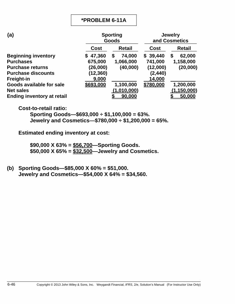
*PROBLEM 6-11A (a) Sporting
Goods Jewelry
and Cosmetics Cost Retail Cost Retail Beginning inventory $ 47,360 $ 74,000 $ 39,440 $ 62,000 Purchases 675,000 1,066,000 741,000 1,158,000 Purchase returns (26,000) (40,000) (12,000) (20,000) Purchase discounts (12,360) (2,440) Freight-in 9,000 14,000 Goods available for sale $693,000 1,100,000 $780,000 1,200,000 Net sales (1,010,000) (1,150,000) Ending inventory at retail $ 90,000 $ 50,000 Cost-to-retail ratio: Sporting Goods—$693,000 ÷ $1,100,000 = 63%. Jewelry and Cosmetics—$780,000 ÷ $1,200,000 = 65%. Estimated ending inventory at cost: $90,000 X 63% = $56,700—Sporting Goods. $50,000 X 65% = $32,500—Jewelry and Cosmetics.
(b) Sporting Goods—$85,000 X 60% = $51,000. Jewelry and Cosmetics—$54,000 X 64% = $34,560.

Copyright © 2013 John Wiley & Sons, Inc. Weygandt Financial, IFRS, 2/e, Solution’s Manual (For Instructor Use Only) 6-47
*PROBLEM 6-12A
Cost of Goods Available for SaleDate Explanation Units Unit Cost Total CostOctober 1 Beginning Inventory 60 €24 €1,440 9 Purchase 120 26 3,120 17 Purchase 70 27 1,890 25 Purchase 80 28 2,240
Total 330 €8,690 Ending Inventory in Units: Units available for sale 330 Sales (100 + 65 + 120) 285 Units remaining in ending inventory
LIFO Ending Inventory October 1 45 @ €24 = €1,080
45

6-48 Copyright © 2013 John Wiley & Sons, Inc. Weygandt Financial, IFRS, 2/e, Solution’s Manual (For Instructor Use Only)
PROBLEM 6-1B (a) The sale will be recorded on February 26. The goods (cost, $800) should
be excluded from Banff’s February 28 inventory. (b) Banff owns the goods once they are shipped on February 26. Include
inventory of $480. (c) Include $720 in inventory. (d) Exclude the items from Banff inventory. Title remains with the
consignor. (e) Title of the goods does not transfer to Banff until March 2. Exclude
this amount from the February 28 inventory. (f) Title to the goods transferred to the customer on February 28. The $200
cost should be excluded from Banff’s February 28 inventory.

Copyright © 2013 John Wiley & Sons, Inc. Weygandt Financial, IFRS, 2/e, Solution’s Manual (For Instructor Use Only) 6-49
PROBLEM 6-2B
(a) COST OF GOODS AVAILABLE FOR SALE Date Explanation Units Unit Cost Total Cost Oct. 1 Beginning Inventory 2,000 £7 £ 14,000 3 Purchase 3,000 8 24,000 9 Purchase 5,500 9 49,500 19 Purchase 4,000 10 40,000 25 Purchase 2,000 11 22,000 Total 16,500 £149,500 (b) FIFO (1) Ending Inventory (2) Cost of Goods Sold
Date
Units Unit
CostTotal Cost
Cost of goods available for sale
£149,500
Oct. 25 2,000 £11 £22,000 Less: Ending inventory 32,00019 1,000 10 10,000
3,000* £32,000 Cost of goods sold £117,500
*16,500 – 13,500 = 3,000
Proof of Cost of Goods SoldDate Units Unit Cost Total Cost Oct. 1 2,000 £7 £14,000
3 3,000 8 24,0009 5,500 9 49,500
19 3,000 10 30,000 13,500 £117,500

6-50 Copyright © 2013 John Wiley & Sons, Inc. Weygandt Financial, IFRS, 2/e, Solution’s Manual (For Instructor Use Only)
PROBLEM 6-2B (Continued)
AVERAGE COST (1) Ending Inventory (2) Cost of Goods Sold £149,500 ÷ 16,500 = £9.0606 Cost of goods available
for sale
£149,500 Units Unit Cost Total Cost Less: Ending inventory 27,182
3,000 £9.0606 £27,182 Cost of goods sold £122,318
Proof of Cost of Goods Sold 13,500 units X £9.0606 = $122,318 (c) (1) FIFO results in the higher inventory amount for the statement of
financial position, £32,000. (2) Average-cost results in the higher cost of goods sold, £122,317.

Copyright © 2013 John Wiley & Sons, Inc. Weygandt Financial, IFRS, 2/e, Solution’s Manual (For Instructor Use Only) 6-51
PROBLEM 6-3B (a) COST OF GOODS AVAILABLE FOR SALE Date Explanation Units Unit Cost Total Cost 1/1 Beginning Inventory 100 $21 $ 2,100 3/15 Purchase 300 24 7,200 7/20 Purchase 200 25 5,000 9/4 Purchase 300 28 8,400 12/2 Purchase 100 30 3,000 Total 1,000 $25,700 (b) FIFO (1) Ending Inventory (2) Cost of Goods Sold
Date
Units Unit
Cost Total Cost
Cost of goods available for sale
$25,700
12/2 100 $30 $3,000 Less: Ending inventory 8,6009/4 200 28 5,600
300 $8,600 Cost of goods sold $17,100
Proof of Cost of Goods Sold Date
Units
Unit Cost
Total Cost
1/1 100 $21 $ 2,1003/15 300 24 7,2007/20 200 25 5,0009/4 100 28 2,800
700 $17,100

6-52 Copyright © 2013 John Wiley & Sons, Inc. Weygandt Financial, IFRS, 2/e, Solution’s Manual (For Instructor Use Only)
PROBLEM 6-3B (Continued) AVERAGE COST (1) Ending Inventory (2) Cost of Goods Sold $25,700 ÷ 1,000 = $25.70 Cost of goods available
for sale
$25,700 Units Unit Cost Total Cost Less: Ending inventory 7,710
300 $25.70 $7,710 Cost of goods sold $17,990
Proof of Cost of Goods Sold 700 units X $25.70 = $17,990 (c) (1) FIFO results in the higher inventory amount, $8,600, as shown in
(b) above. (2) Average-cost produces the higher cost of goods sold, $17,990 as
shown in (b) above.

Copyright © 2013 John Wiley & Sons, Inc. Weygandt Financial, IFRS, 2/e, Solution’s Manual (For Instructor Use Only) 6-53
PROBLEM 6-4B
(a) MUNICH COMPANY Condensed Income Statements For the Year Ended December 31, 2014
FIFO Average-cost
Sales revenue .......................................... €780,000 €780,000 Cost of goods sold Beginning inventory ......................... 16,000 16,000 Cost of goods purchased ................. 480,500 480,500 Cost of goods available for sale ...... 496,500 496,500 Ending inventory ............................... 40,500a 36,690b Cost of goods sold ........................... 456,000 459,810 Gross profit .............................................. 324,000 320,190 Operating expenses ................................ 130,000 130,000 Income before income taxes .................. 194,000 190,190 Income tax expense (36%) ...................... 69,840 68,468 Net income ............................................... €124,160 €121,722
a15,000 X €2.70 = €40,500. b€496,500 ÷ 203,000=€2.446 per unit; 15,000 × €2.446=€36,690
(b) (1) The FIFO method produces the more meaningful inventory amount for the statement of financial position because the units are costed at the most recent purchase prices.
(2) The FIFO method is more likely to approximate actual physical
flow because the oldest goods are usually sold first to minimize spoilage and obsolescence.
(3) There will be €1,372 additional cash available under average-cost
because income taxes are €68,468 under average-cost and €69,840 under FIFO.

6-54 Copyright © 2013 John Wiley & Sons, Inc. Weygandt Financial, IFRS, 2/e, Solution’s Manual (For Instructor Use Only)
PROBLEM 6-5B
(a) Cost of Goods Available for Sale Date Explanation Units Unit Cost Total Cost June 1 Beginning Inventory 40 $40 $ 1,600 June 4 Purchase 135 43 5,805 June 18 Purchase 55 46 2,530 June 18 Purchase return (10) 46 (460) June 28 Purchase 30 50 1,500 Total 250 $10,975 Ending Inventory in Units: Sales Revenue Units available for sale 250 Unit Sales (110 – 15 + 60) 155 Date Units Price Total SalesUnits remaining in ending inventory 95 June 10 110 $70 $ 7,700 11 (15) 70 (1,050) 25 60 75 4,500 155 $11,150
(1) FIFO (i) Ending Inventory (ii) Cost of Goods Sold June 28
18 30 @ $50
45 @ $46 $1,500
2,070 Cost of goods available for sale
$10,975
4 20 @ $43 860 Less: Ending inventory 4,430 95 $4,430 Cost of goods sold $ 6,545 (iii) Gross Profit (iv) Gross Profit RateSales revenue $11,150 Gross profit $ 4,605 = 41.3% Cost of goods sold 6,545 Net sales $11,150Gross profit $ 4,605

Copyright © 2013 John Wiley & Sons, Inc. Weygandt Financial, IFRS, 2/e, Solution’s Manual (For Instructor Use Only) 6-55
PROBLEM 6-5B (Continued)
(2) Average-Cost Weighted-average cost per unit: Cost of goods available for sale
Units available for sale $10,975 = $43.90 250 (i) Ending Inventory (ii) Cost of Goods Sold
95 units @ $43.90 $4,170.50 Cost of goods available for sale $10,975.00
Less: Ending inventory 4,170.50 Cost of goods sold $ 6,804.50 (iii) Gross Profit (iv) Gross Profit Rate Sales revenue $11,150.00 Gross profit $ 4,345.50 = 39% Cost of goods sold 6,804.50 Net sales $11,150.00Gross profit $ 4,345.50
(b) In this period of rising prices, average-cost gives the higher cost of goods sold and the lower gross profit. FIFO gives the lower cost of goods sold and the higher gross profit.

6-56 Copyright © 2013 John Wiley & Sons, Inc. Weygandt Financial, IFRS, 2/e, Solution’s Manual (For Instructor Use Only)
PROBLEM 6-6B
(a) GAS GUZZLERS Income Statement (partial) For the Year Ended December 31, 2014 (1) Specific
Identification (2) FIFO (3) Average-
cost Sales revenuea $9,185 $9,185 $9,185 Beginning inventory 1,320 1,320 1,320 Purchasesb 6,505 6,505 6,505 Cost of goods available
for sale 7,825 7,825
7,825 Ending inventoryc 2,500 2,720 2,450 Cost of goods sold 5,325 5,105 5,375 Gross profit $3,860 $4,080 $3,810
(a)(2,200 @ $1.05) + (5,500 @ $1.25) (b)(2,500 @ $.65) + (4,000 @ $.72) + (2,500 @ $.80) (c)Specific identification ending inventory consists of:
Beginning inventory (2,200 liters – 1,100 – 450) 650 @ $.60 $ 390.00March 3 purchase (2,500 liters – 1,100 – 850) 550 @ $.65 357.50March 10 purchase (4,000 liters – 2,900) 1,100 @ $.72 792.00March 20 purchase (2,500 liters – 1,300) 1,200 @ $.80 960.00 3,500 liters $2,499.50
FIFO ending inventory consists of:
March 20 purchase 2,500 @ $.80 $2,000March 10 purchase 1,000 @ $.72 720 3,500 liters $2,720
Average-cost ending inventory consists of: 3,500 liters @ $.70 = $2,450 Weighted-average cost per liter: 7,825 .
(2,200 + 2,500 + 4,000 + 2,500) = $.70 per liter (b) Companies can choose a cost flow method that produces the highest
possible cost of goods sold and lowest gross profit to justify price increases. In this example, Average-cost produces the lowest gross profit and best support to increase selling prices.

Copyright © 2013 John Wiley & Sons, Inc. Weygandt Financial, IFRS, 2/e, Solution’s Manual (For Instructor Use Only) 6-57
PROBLEM 6-7B
(a) AAR CO. Condensed Income Statement For the Year Ended December 31, 2014
FIFO Average-cost
Sales revenue ............................................ CHF740,000 CHF740,000 Cost of goods sold Beginning inventory .......................... 47,000 47,000 Cost of goods purchased .................. 532,000 532,000 Cost of goods available for sale ....... 579,000 579,000 Ending inventory ................................ 140,000a 131,600b Cost of goods sold ............................. 439,000 447,400 Gross profit ................................................ 301,000 292,600 Operating expenses .................................. 140,000 140,000 Income before income taxes .................... 161,000 152,600 Income tax expense (32%) ........................ 51,520 48,832 Net income ................................................. CHF109,480 CHF103,768
a(25,000 @ CHF5.60) = CHF140,000. b(CHF579,000 ÷ 110,000 units=CHF5.264 per unit; 25,000 @ CHF5.264=CHF131,600 (b) Answers to questions: (1) The FIFO method produces the more meaningful inventory
amount for the statement of financial position because the units are costed at the most recent purchase prices.
(2) The FIFO method is more likely to approximate actual physical flow
because the oldest goods are usually sold first to minimize spoilage and obsolescence.
(3) There will be CHF2,688 additional cash available under average-
cost because income taxes are CHF48,832 under average-cost and CHF51,520 under FIFO.
6-58 Copyright © 2013 John Wiley & Sons, Inc. Weygandt Financial, IFRS, 2/e, Solution’s Manual (For Instructor Use Only)
*PROBLEM 6-8B
(a) Sales:
January 8 110 units @ $28 $3,080 January 10 (return) (10 units @ $28) (280)January 20 80 units @ $32 2,560
180 units $5,360 (1) FIFO Date Purchases Cost of Goods Sold Balance January 1 (100 @ $14) $1,400 January 5 (150 @ $17) $2,550 (100 @ $14) } $3,950 (150 @ $17) January 8 (100 @ $14) } $1,570 (140 @ $17) $2,380 ( 10 @ $17) January 10 (–10 @ $17) ($ 170) (150 @ $17) $2,550 January 15 ( 55 @ $19) $1,045 (150 @ $17) } $3,595 ( 55 @ $19) January 16 ( –5 @ $19)($ 95) (150 @ $17) } $3,500 ( 50 @ $19) January 20 (80 @ $17) $1,360 ( 70 @ $17)
( 50 @ $19) } $2,140
January 25
( 30 @ $22) $ 660 ( 70 @ $17)
( 50 @ $19) } $2,800 ( 30 @ $22) $2,760
(i) Cost of goods sold = $2,760. (ii) Ending inventory = $2,800. (iii) Gross
profit = $5,360 – $2,760 = $2,600.

Copyright © 2013 John Wiley & Sons, Inc. Weygandt Financial, IFRS, 2/e, Solution’s Manual (For Instructor Use Only) 6-59
*PROBLEM 6-8B (Continued) (2) Moving-Average Cost Date Purchases Cost of Goods Sold Balance January 1 (100 @ $14) $1,400 January 5 (150 @ $17) $2,550 (250 @ $15.80)a $3,950 January 8 (110 @ $15.80) $1,738 (140 @ $15.80) $2,212 January 10 (–10 @ $15.80) ($ 158) (150 @ $15.80) $2,370 January 15 ( 55 @ $19) $1,045 (205 @ $16.659)b $3,415 January 16 ( –5 @ $19) ($ 95) (200 @ $16.60)c $3,320 January 20 ( 80 @ $16.60) $1,328 (120 @ $16.60) $1,992 January 25 ( 30 @ $22) $ 660 (150 @ $17.68)d $2,652
$2,908
*rounded a$3,950 ÷ 250 = $15.80 c$3,320 ÷ 200 = $16.60 b$3,415 ÷ 205 = $16.659 d$2,652 ÷ 150 = $17.68
(i) Cost of goods sold = $2,908. (ii) Ending inventory = $2,652. (iii) Gross
profit = $5,360 – $2,908 = $2,452. (b) FIFO Moving-Average CostSales $5,360 $5,360 Cost of goods sold 2,760 2,908 Gross profit $2,600 $2,452 Ending inventory $2,800 $2,652 In a period of rising costs, the moving-average cost flow assumption results in the higher cost of goods sold and lower gross profit. FIFO gives the lower cost of goods sold and higher gross profit.
On the statement of financial position, FIFO gives the higher ending inventory (representing the most current costs); and moving-average cost results in the lower ending inventory.

6-60 Copyright © 2013 John Wiley & Sons, Inc. Weygandt Financial, IFRS, 2/e, Solution’s Manual (For Instructor Use Only)
*PROBLEM 6-9B
(a) (1)
FIFO Date Purchases Cost of Goods Sold Balance July 1 (5 @ HK$120) HK$ 600 (5 @ HK$120) HK$ 600 6 (3 @ HK$120) HK$360 (2 @ HK$120) HK$ 240 11 (6 @ HK$136) HK$ 816 (2 @ HK$120) }HK$1,056 (6 @ HK$136)
14 (2 @ HK$120) } HK$512
(2 @ HK$136) (4 @ HK$136) HK$ 544
21
(8 @ HK$147)
HK$1,176 (4 @ HK$136) }HK$1,720
(8 @ HK$147) 27 (4 @ HK$136)
(2 @ HK$147) } HK$838
(6 @ HK$147) HK$ 882 (2) MOVING-AVERAGE COST Date Purchases Cost of Goods Sold Balance July 1 (5 @ HK$120) HK$ 600 ( 5 @ HK$120) HK$ 600 6 (3 @ HK$120) HK$360 ( 2 @ HK$120) HK$ 240 11 (6 @ HK$136) HK$ 816 ( 8 @ HK$132)* HK$1,056 14 (4 @ HK$132) HK$528 ( 4 @ HK$132) HK$ 528 21 (8 @ HK$147) HK$1,176 (12 @ HK$142)** HK$1,704 27 (6 @ HK$142) HK$852 ( 6 @ HK$142) HK$ 852
* HK$1,056 ÷ 8 = HK$132
** HK$1,704 ÷ 12 = HK$142 (b) The higher ending inventory is HK$882 under the FIFO method.

Copyright © 2013 John Wiley & Sons, Inc. Weygandt Financial, IFRS, 2/e, Solution’s Manual (For Instructor Use Only) 6-61
*PROBLEM 6-10B
(a) November Net sales ....................................................... $600,000 Cost of goods sold Beginning inventory ............................ $ 30,000 Purchases ............................................. $368,000 Less: Purchase returns and allowances ................................ 13,300 Purchase discounts ................. 8,500 Add: Freight-in ................................... 4,800 Cost of goods purchased ................... 351,000 Cost of goods available for sale ......... 381,000 Ending inventory ................................. 33,000 Cost of goods sold ....................... 348,000 Gross profit .................................................. $252,000 Gross profit rate = $252,000 = 42% $600,000
(b) Net sales ................................................. $700,000 Less: Estimated gross profit (42% X $700,000) ........................ 294,000 Estimated cost of goods sold ............... $406,000 Beginning inventory .............................. $ 33,000 Purchases ............................................... $420,000 Less: Purchase returns and allowances .................................. $14,900 Purchase discounts ................... 9,500 24,400 Net purchases ........................................ 395,600 Freight-in ................................................ 5,900 Cost of goods purchased ..................... 401,500 Cost of goods available for sale ........... 434,500 Less: Estimated cost of goods sold .............................................. 406,000 Estimated inventory lost in fire ............ $ 28,500

6-62 Copyright © 2013 John Wiley & Sons, Inc. Weygandt Financial, IFRS, 2/e, Solution’s Manual (For Instructor Use Only)
*PROBLEM 6-11B
(a) Hardcovers Paperbacks Cost Retail Cost Retail Beginning inventory € 420,000 € 700,000 € 280,000 € 360,000 Purchases 2,094,000 3,200,000 1,155,000 1,540,000 Freight-in 26,000 12,000 Purchase discounts (44,000) (22,000) Goods available for sale €2,496,000 3,900,000 €1,425,000 1,900,000 Net sales 3,100,000 1,570,000 Ending inventory at retail € 800,000 € 330,000 Cost-to-retail ratio: Hardcovers—€2,496,000 ÷ €3,900,000 = 64%. Paperbacks—€1,425,000 ÷ €1,900,000 = 75%. Estimated ending inventory at cost: €800,000 X 64% = €512,000—Hardcovers. €330,000 X 75% = €247,500—Paperbacks.
(b) Hardcovers—€790,000 X 65% = €513,500. Paperbacks—€335,000 X 77% = €257,950.

Copyright © 2013 John Wiley & Sons, Inc. Weygandt Financial, IFRS, 2/e, Solution’s Manual (For Instructor Use Only) 6-63
*PROBLEM 6-12B Cost of Goods Available for Sale Date Explanation Units Unit Cost Total Cost June 1 Beginning Inventory 40 $40 $ 1,600 June 4 Purchase 135 43 5,805 June 18 Purchase 55 46 2,530 June 18 Purchase return (10) 46 (460) June 28 Purchase 30 50 1,500 Total 250 $10,975 Ending Inventory in Units: Units available for sale 250 Sales (110 – 15 + 60) 155 Units remaining in ending inventory 95
LIFO Ending Inventory June 1 40 @ $40 $1,600 4 55 @ 43 2,365 95 $3,965

6-64 Copyright © 2013 John Wiley & Sons, Inc. Weygandt Financial, IFRS, 2/e, Solution’s Manual (For Instructor Use Only)
COMPREHENSIVE PROBLEM SOLUTION
(a) Dec. 3 Inventory (4,000 X $0.72) ...........................
Accounts Payable ............................... 2,880
2,880 5 Accounts Receivable (4,400 X $0.92) .......
Sales Revenue .................................... Cost of Good Sold ...................................... Inventory (3,000 X $0.65) + (1,400 X $0.72) ..................................
4,048
2,958
4,048
2,958 7 Sales Returns and Allowances .................
Accounts Receivable ......................... Inventory ..................................................... Cost of Good Sold ..............................
184
144
184
144 17 Inventory (2,200 X $0.78) ...........................
Cash ..................................................... 1,716
1,716 22 Accounts Receivable (2,000 X $0.95) .......
Sales Revenue .................................... Cost of Goods Sold (2,000 X $0.72) .......... Inventory .............................................
1,900
1,440
1,900
1,440 31 Salaries and Wages Expense....................
Salaries and Wages Payable ............. Depreciation Expense ................................ Accumulated Depreciation— Equipment ........................................
400
200
400
200

Copyright © 2013 John Wiley & Sons, Inc. Weygandt Financial, IFRS, 2/e, Solution’s Manual (For Instructor Use Only) 6-65
COMPREHENSIVE PROBLEM SOLUTION (Continued) (b) General Ledger
Cash Bal. 4,650 1,716Bal. 2,934
Inventory Bal. 1,950 2,880 144 1,716
2,958 1,440
Bal. 2,292
Accounts Payable Bal. 3,000
2,880 Bal. 5,880
Salaries and Wages Payable 400 Bal. 400
Sales Revenue 4,048
1,900 Bal. 5,948
Cost of Goods Sold 2,958 1,440
144
Bal. 4,254
Depreciation Expense 200 Bal. 200
Accounts ReceivableBal. 3,900 4,048 1,900
184
Bal. 9,664
EquipmentBal. 21,000
Accumulated Depreciation—Equipment
Bal. 1,500 200 Bal. 1,700
Share Capital—Ordinary
Bal. 20,000
Retained Earnings
Bal. 7,000
Salaries and Wages Expense
400 Bal. 400
Sales Returns & Allowances184
Bal. 184
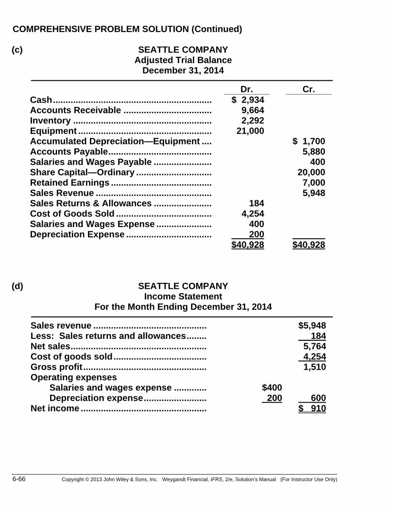
6-66 Copyright © 2013 John Wiley & Sons, Inc. Weygandt Financial, IFRS, 2/e, Solution’s Manual (For Instructor Use Only)
COMPREHENSIVE PROBLEM SOLUTION (Continued) (c) SEATTLE COMPANY Adjusted Trial Balance December 31, 2014
Dr. Cr. Cash ............................................................... $ 2,934Accounts Receivable ................................... 9,664Inventory ....................................................... 2,292Equipment ..................................................... 21,000Accumulated Depreciation—Equipment .... $ 1,700Accounts Payable ......................................... 5,880Salaries and Wages Payable ....................... 400Share Capital—Ordinary .............................. 20,000Retained Earnings ........................................ 7,000Sales Revenue .............................................. 5,948Sales Returns & Allowances ....................... 184Cost of Goods Sold ...................................... 4,254Salaries and Wages Expense ...................... 400Depreciation Expense .................................. 200 $40,928 $40,928
(d) SEATTLE COMPANY Income Statement For the Month Ending December 31, 2014
Sales revenue ............................................. $5,948Less: Sales returns and allowances........ 184Net sales ...................................................... 5,764Cost of goods sold ..................................... 4,254Gross profit ................................................. 1,510Operating expenses Salaries and wages expense ............. $400 Depreciation expense ......................... 200 600Net income .................................................. $ 910

Copyright © 2013 John Wiley & Sons, Inc. Weygandt Financial, IFRS, 2/e, Solution’s Manual (For Instructor Use Only) 6-67
COMPREHENSIVE PROBLEM SOLUTION (Continued) SEATTLE COMPANY Statement of Financial Position December 31, 2014
Assets
Property, plant, and equipment Equipment .............................................. $21,000 Less: Accumulated depreciation— Equipment .................................. 1,700 $19,300
Current assets Inventory ................................................ 2,292 Accounts receivable.............................. 9,664 Cash ........................................................ 2,934 14,890Total assets ................................................... $34,190
Equity and liabilities
Equity Share capital—ordinary ........................ $20,000 Retained earnings ($7,000 + $910)....... 7,910 $27,910 Current liabilities Accounts payable.................................. 5,880 Salaries and wages payable ................. 400 6,280Total equity and liabilities ............................ $34,190

6-68 Copyright © 2013 John Wiley & Sons, Inc. Weygandt Financial, IFRS, 2/e, Solution’s Manual (For Instructor Use Only)
COMPREHENSIVE PROBLEM SOLUTION (Continued) (e) FIFO Method
Units Unit Cost
Cost of Goods Available for Sale
Beg. Inventory 3,000 $0.65 $1,950 Dec. 3 purchase. 4,000 $0.72 2,880 Dec. 17 purchase. 2,200 $0.78 1,716 9,200 $6,546
Ending Inventory Cost of Goods Sold Dec. 17 2,200 X $0.78 = $1,716 Cost of goods available for sale $6,546Dec. 3 800* X $0.72 = 576 Less: Ending inventory 2,292 3,000 $2,292 Cost of goods sold $4,254
*(9,200 – 4,400 + 200 – 2,000) – 2,200 (f) Average-cost Method
Weighted-average cost per unit $6,546 = $.712/unit 9,200 units
Ending Inventory Cost of Goods Sold 3,000 X $0.712 = $2,136 Cost of goods available for sale $6,546 Less: Ending inventory 2,136 Cost of goods sold $4,410

Copyright © 2013 John Wiley & Sons, Inc. Weygandt Financial, IFRS, 2/e, Solution’s Manual (For Instructor Use Only) 6-69
CCC6 CONTINUING COOKIE CHRONICLE (a) COST OF GOODS AVAILABLE FOR SALE Date Explanation Units Unit Cost Total CostFeb. 1 Beginning Inventory 3 $595 $1,785Feb. 2 Purchase 2 600 1,200Mar. 2 Purchase 1 618 618Apr. 1 Purchase 2 612 1,224May 4 Purchase 3 625 1,875 Total 11 $6,702
FIFO
Ending Inventory Cost of Goods Sold
Date Units Unit
Cost Total
Cost Cost of goods available for sale $6,702
May 4 3 $625 $1,875 Less: Ending inventory 2,487Apr. 1 1 612 612 Cost of goods sold $4,215 4 $2,487
Gross Profit Gross Profit RateSales $8,050 $3,835 47.64%Less: Cost of goods sold 4,215 $8,050 Gross profit $3,835
Average Cost
Ending Inventory Cost of Goods Sold
$6,702/11 = $609.273 Cost of goods available for sale $6,702.00
Less: Ending inventory 2,437.09 Units
Unit Cost
Total Cost
Cost of goods sold $4,264.91
4 $609.273 $2,437.09
Gross Profit Gross Profit Rate
Sales $8,050.00 $3,785.09 47.02%Less: Cost of goods sold 4,264.91 $8,050.00 Gross profit $3,785.09

6-70 Copyright © 2013 John Wiley & Sons, Inc. Weygandt Financial, IFRS, 2/e, Solution’s Manual (For Instructor Use Only)
BYP 6-1 FINANCIAL REPORTING PROBLEM
(a) December 31, 2010 December 26, 2009 Inventories W13,364,524 million W9,839,329million
(b) Won change in inventories between 2009 and 2010: W13,364,524 – W9,839,329 = W3,525,195 million increase Percent change in inventories between 2009 and 2010: W3,525,195 ÷ W9,839,329 = 35.8% increase 2010 inventory as a percent of current assets: W13,364,524 ÷ W61,402,589 = 21.8%
(c) Inventories are valued at lower of cost or net realizable value. Cost is determined using the average-cost method. (See Note 2.8).
(d) Samsung (in millions) 2010 2009 Cost of Goods Sold W102,666,824 W94,594,863
2010 cost of goods sold as a percent of sales: W102,666,824 ÷ W154,630,328 = 66.4%

Copyright © 2013 John Wiley & Sons, Inc. Weygandt Financial, IFRS, 2/e, Solution’s Manual (For Instructor Use Only) 6-71
BYP 6-2 COMPARATIVE ANALYSIS PROBLEM
(a) (1) Inventory turnover:
Nestlé: CHF45,849 ÷ CHF7,925 + CHF7,734 = 5.9 times 2
Zetar: £107,677 ÷ £16,453 + £16,039 = 6.6 times 2 (2) Days in inventory: Nestlé: 365 ÷ 5.9 = 62 days Zetar: 365 ÷ 6.6 = 55 days
(b) Zetar’s turnover of 6.6 times is approximately 12% higher than Nestlé’s 5.9 times, resulting in days in inventory of 55 versus 62. Thus, Zetar’s inventory control is more effective.

6-72 Copyright © 2013 John Wiley & Sons, Inc. Weygandt Financial, IFRS, 2/e, Solution’s Manual (For Instructor Use Only)
BYP 6-3 REAL-WORLD FOCUS The following responses are based on the 2011 annual report: (a) $1,486,000,000, as of July 30, 2011. (b) $1,486,000,000 – $1,327,000,000 = $159,000,000 increase. (c) 64.7 percent ($962 ÷ $1,486). (d) Lower of cost or market using standard cost, which approximates FIFO.

Copyright © 2013 John Wiley & Sons, Inc. Weygandt Financial, IFRS, 2/e, Solution’s Manual (For Instructor Use Only) 6-73
BYP 6-4 DECISION-MAKING ACROSS THE ORGANIZATION (a) (1) Sales January 1–March 31 .................... $180,000 Cash sales 4/1–4/10 ($20,500 X 40%) ... 8,200 Acknowledged credit sales 4/1–4/10 .... 37,000 Sales made but unacknowledged ......... 5,600 Sales as of April 10 ................................ $230,800 (2) Purchases January 1–March 31 ............ $ 94,000 Cash purchases 4/1–4/10 ...................... 4,200 Credit purchases 4/1–4/10 ..................... $12,400 Less: Items in transit ............................ 1,900 10,500 Purchases as of April 10 ....................... $108,700 *(b) 2013 2012
Net sales ........................................................ $600,000 $480,000 Cost of goods sold Inventory, January 1 .............................. 60,000 40,000 Cost of goods purchased ...................... 404,000 346,400 Cost of goods available for sale ........... 464,000 386,400 Inventory, December 31 ........................ 80,000 60,000 Cost of goods sold ................................ 384,000 326,400 Gross profit .................................................... $216,000 $153,600 Gross profit rate ............................................. 36% 32% Average gross profit rate ...................... 34%
*(c) Sales (from (a) (1)) ......................................... $230,800 Less: Gross profit ($230,800 X 34%) ........... 78,472 Cost of goods sold ........................................ $152,328 Inventory, January 1 ...................................... $ 80,000 Purchases (from (a) (2)) ................................ 108,700 Cost of goods available for sale ................... 188,700 Cost of goods sold ........................................ 152,328 Estimated inventory at time of fire ............... 36,372 Less: Inventory salvaged ............................. 17,000 Estimated inventory loss .............................. $ 19,372

6-74 Copyright © 2013 John Wiley & Sons, Inc. Weygandt Financial, IFRS, 2/e, Solution’s Manual (For Instructor Use Only)
BYP 6-5 COMMUNICATION ACTIVITY
MEMO
To: Kathy McDonnell, President From: Student Re: 2013 ending inventory error
As you know, 2013 ending inventory was overstated by $1 million. Of course, this error will cause 2013 net income to be incorrect because the ending inventory is used to compute 2013 cost of goods sold. Since the ending inven-tory is subtracted in the computation of cost of goods sold, an overstatement of ending inventory results in an understatement of cost of goods sold and therefore an overstatement of net income. Unfortunately, unless corrected, this error will also affect 2014 net income. The 2013 ending inventory is also the 2014 beginning inventory. Therefore, 2014 beginning inventory is also overstated, which causes an overstatement of cost of goods sold and an understatement of 2014 net income.

Copyright © 2013 John Wiley & Sons, Inc. Weygandt Financial, IFRS, 2/e, Solution’s Manual (For Instructor Use Only) 6-75
BYP 6-6 ETHICS CASE
(a) The higher cost of the items ordered, received, and on hand at year-
end will increase the weighted average cost per unit used to calculate cost of goods sold, thereby lowering current year’s income and income taxes. If the purchase at year-end had been made in the next year, the next year’s cost of goods sold would have absorbed the higher cost. Next year’s income will be increased if unit purchases (next year) are less than unit sales (next year). This is because the lower costs carried from the earlier year as inventory will be charged to next year’s cost of goods sold. Therefore, next year’s income taxes will increase.
(b) No. The president would not have given the same directive because the
purchase under FIFO would have had no effect on net income of the current year.
(c) The accountant has no grounds for not ordering the goods if the
president insists. The purchase is legal and ethical.

6-76 Copyright © 2013 John Wiley & Sons, Inc. Weygandt Financial, IFRS, 2/e, Solution’s Manual (For Instructor Use Only)
GAAP EXERCISES
GAAP6-1 Key Similarities are (1) the definitions for inventory are essentially the same, (2) the guidelines on who owns the goods—goods in transit, consigned goods, and the costs to include in inventory are essentially accounted for the same under IFRS and U.S. GAAP; (3) use of specific identification cost flow assumption, where appropriate; (4) unlike property, plant, and equipment, IFRS does not permit the option of valuing inventories at fair value. Key differences are related to (1) the LIFO cost flow assumption—U.S. GAAP permits the use of LIFO for inventory valuation, but IFRS prohibits its use. FIFO and average-cost are the only two acceptable cost flow assumptions permitted under IFRS; (2) lower-of-cost-or-market test for inventory valuation—IFRS defines market as net realizable value. U.S. GAAP on the other hand defines market as replacement cost; (3) inventory write-downs—under U.S. GAAP, if inventory is written down under the lower-of-cost-or-market valuation, the new basis is now considered its cost. As a result, the inventory may not be written back up to its original cost in a subsequent period. Under IFRS, the write-down may be reversed in a subsequent period up to the amount of the previous write-down. Both the write-down and any subsequent reversal should be reported on the income statement; (4) IFRS requires pre-harvest inventories of agricultural products to be reported at fair value less cost of disposal. GAAP requires these items to be recorded at cost; (5) The requirements for accounting and reporting for inventories are more principles-based under IFRS. That is, U.S. GAAP provides more detailed guidelines for inventory accounting. GAAP6-2 Under IFRS, LaTour’s inventory turnover ratio is computed as follows: Cost of Goods Sold/Average Inventory €578/ €154 = 3.75 or approximately 97 days (365 ÷ 3.75). Difficulties in comparison to a company using U.S. GAAP could arise if the U.S. company uses the LIFO cost flow assumption, which is prohibited under IFRS. Generally, in times of rising prices, LIFO results in a lower inventory balance reported on the balance sheet (assumes more recently purchased items are sold first). Thus, the U.S. GAAP company will report higher inventory turnover ratios. The LIFO reserve can be used to adjust the reported LIFO numbers to FIFO and to permit an “apples to apples” comparison.

Copyright © 2013 John Wiley & Sons, Inc. Weygandt Financial, IFRS, 2/e, Solution’s Manual (For Instructor Use Only) 6-77
GAAP6-3
Item No. Cost Market LCM AB $ 1,700 $ 1,400 $ 1,400 TRX 2,200 2,300 2,200 NWA 7,800 7,100 7,100 SGH 3,000 3,700 3,000 $14,700 $14,500 $13,700

6-78 Copyright © 2013 John Wiley & Sons, Inc. Weygandt Financial, IFRS, 2/e, Solution’s Manual (For Instructor Use Only)
GAAP FINANCIAL REPORTING PROBLEM
GAAP6-4 (a)
Inventories: 2010 2009
Finished goods and work-in-progress $36,935 $35,570
(b) Dollar amount of inventory change: ($36,935 - $35,570) = $1,365 Percent change in inventories from 2009 to 2010:
$36,935 - $35,570 $35,570 = 3.8%
Inventory as a percent of current assets in 2010:
$36,935 $237,591 = 15.5%
(c)
2010 2009 2008
(Product) cost of goods sold $348,313 $318,645 $333,314
(Product) cost of goods sold as percent of net product sales in 2010:
$348,313 $517,149 = 67.4%