Chapter 5a: CPU Scheduling

Silberschatz, Galvin and Gagne ©2018 Operating System Concepts – 10th Edition

Chapter 5a: CPU Scheduling

5a.2 Silberschatz, Galvin and Gagne ©2018 Operating System Concepts – 10th Edition

Outline

Basic Concepts

Scheduling Criteria

Scheduling Algorithms


Objectives

Describe various CPU scheduling algorithms

Assess CPU scheduling algorithms based on scheduling criteria

Explain the issues related to multiprocessor and multicore scheduling

Describe various real-time scheduling algorithms

Describe the scheduling algorithms used in the Windows, Linux, and

Solaris operating systems

Apply modeling and simulations to evaluate CPU scheduling

algorithms


Basic Concepts

Maximum CPU utilization

obtained with multiprogramming

CPU–I/O Burst Cycle – Process

execution consists of a cycle of

CPU execution and I/O wait

CPU burst followed by I/O burst

CPU burst distribution is of main

concern


Histogram of CPU-burst Times

Large number of short bursts Small number of longer bursts


CPU Scheduler

The CPU scheduler selects from among the processes in ready

queue, and allocates a CPU core to one of them

• Queue may be ordered in various ways

CPU scheduling decisions may take place when a process:

1. Switches from running to waiting state

2. Switches from running to ready state

3. Switches from waiting to ready

4. Terminates

For situations 1 and 4, there is no choice in terms of scheduling. A

new process (if one exists in the ready queue) must be selected

for execution.

For situations 2 and 3, however, there is a choice.


Preemptive and Nonpreemptive Scheduling

When scheduling takes place only under circumstances 1 and

4, the scheduling scheme is nonpreemptive.

Otherwise, it is preemptive.

Under Nonpreemptive scheduling, once the CPU has been

allocated to a process, the process keeps the CPU until it

releases it either by terminating or by switching to the waiting

state.

Virtually all modern operating systems including Windows,

MacOS, Linux, and UNIX use preemptive scheduling

algorithms.


Preemptive Scheduling and Race Conditions

Preemptive scheduling can result in race conditions

when data are shared among several processes.

Consider the case of two processes that share data.

While one process is updating the data, it is preempted

so that the second process can run. The second process

then tries to read the data, which are in an inconsistent

state.

This issue will be explored in detail in Chapter 6.


Dispatcher

Dispatcher module gives control of the

CPU to the process selected by the CPU

scheduler; this involves:

• Switching context

• Switching to user mode

• Jumping to the proper location in the

user program to restart that program

Dispatch latency – time it takes for the

dispatcher to stop one process and start

another running


Scheduling Criteria

CPU utilization – keep the CPU as busy as possible

Throughput – # of processes that complete their execution

per time unit

Turnaround time – amount of time to execute a particular

process

Waiting time – amount of time a process has been waiting

in the ready queue

Response time – amount of time it takes from when a

request was submitted until the first response is produced.


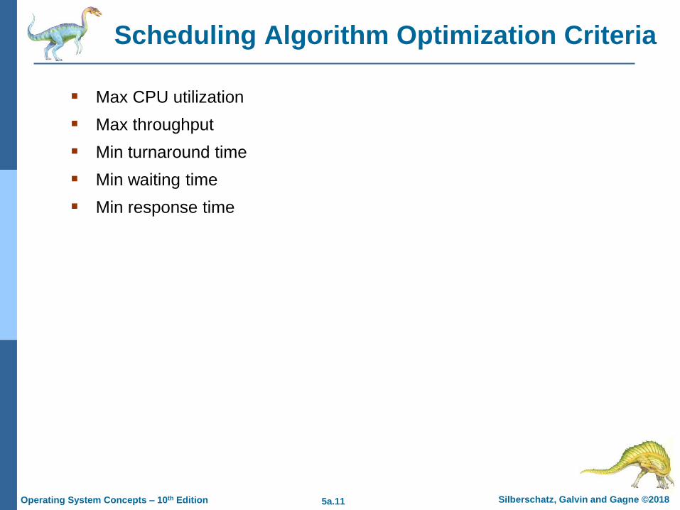
Scheduling Algorithm Optimization Criteria

Max CPU utilization

Max throughput

Min turnaround time

Min waiting time

Min response time


First- Come, First-Served (FCFS) Scheduling

Process Burst Time

P1 24

P2 3

P3 3

Suppose that the processes arrive in the order: P1 , P2 , P3

The Gantt Chart for the schedule is:

Waiting time for P1 = 0; P2 = 24; P3 = 27

Average waiting time: (0 + 24 + 27)/3 = 17

P P P1 2 3

0 24 3027


FCFS Scheduling (Cont.)

Suppose that the processes arrive in the order:

P2 , P3 , P1

The Gantt chart for the schedule is:

Waiting time for P1 = 6; P2 = 0; P3 = 3

Average waiting time: (6 + 0 + 3)/3 = 3

Much better than previous case

Convoy effect - short process behind long process

• Consider one CPU-bound and many I/O-bound processes

P1

0 3 6 30

P2

P3


Shortest-Job-First (SJF) Scheduling

Associate with each process the length of its next CPU burst

• Use these lengths to schedule the process with the shortest time

SJF is optimal – gives minimum average waiting time for a given set

of processes

• The difficulty is knowing the length of the next CPU request

• Could ask the user


Shortest-Job-First (SJF) Scheduling

Associate with each process the length of its next CPU burst

• Use these lengths to schedule the process with the

shortest time

SJF is optimal – gives minimum average waiting time for a

given set of processes

Preemptive version called shortest-remaining-time-first

How do we determine the length of the next CPU burst?

• Could ask the user

• Estimate


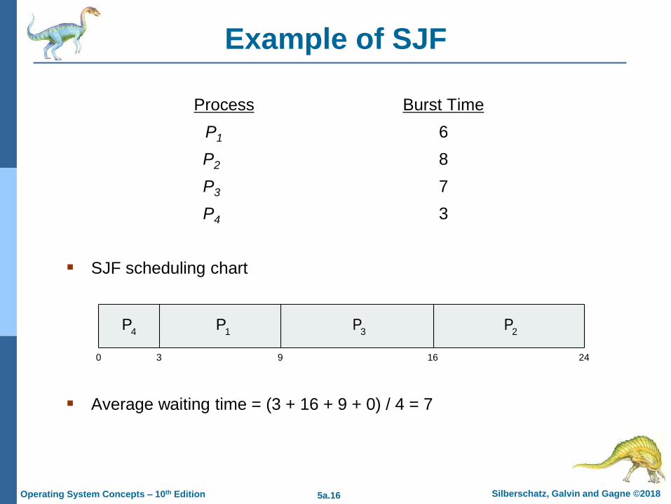
Example of SJF

ProcessArrival Time Burst Time

P1 0.0 6

P2 2.0 8

P3 4.0 7

P4 5.0 3

SJF scheduling chart

Average waiting time = (3 + 16 + 9 + 0) / 4 = 7

P3

0 3 24

P4

P1

169

P2


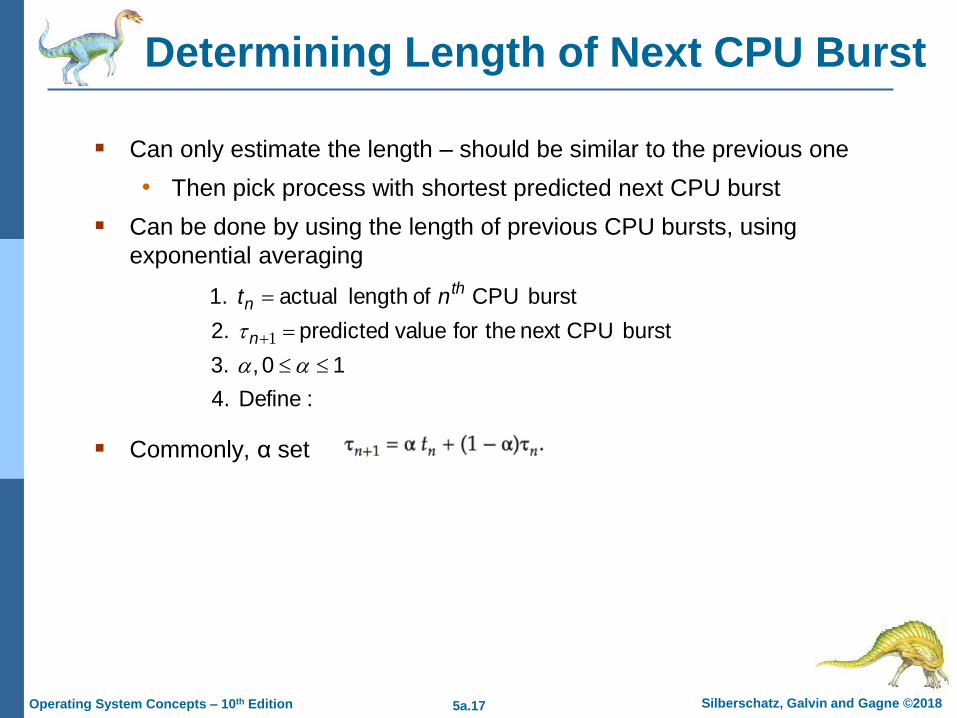
Determining Length of Next CPU Burst

Can only estimate the length – should be similar to the previous one

• Then pick process with shortest predicted next CPU burst

Can be done by using the length of previous CPU bursts, using

exponential averaging

Commonly, α set to ½

:Define 4.

10 , 3.

burst CPU next the for value predicted 2.

burst CPU of length actual 1.

1n

thn nt


Prediction of the Length of the Next CPU Burst


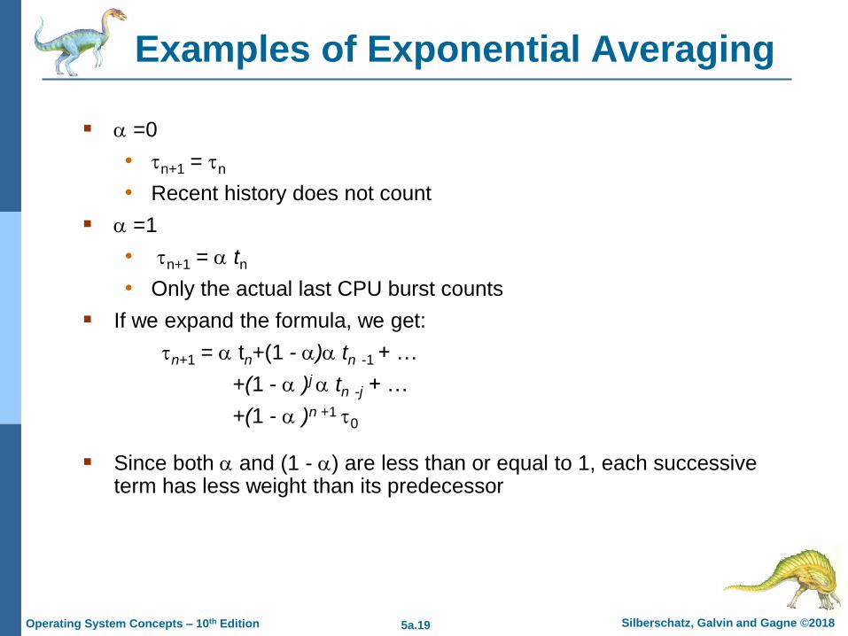
Examples of Exponential Averaging

=0

• n+1 = n

• Recent history does not count

=1

• n+1 = tn

• Only the actual last CPU burst counts

If we expand the formula, we get:

n+1 = tn+(1 - ) tn -1 + …

+(1 - )j tn -j + …

+(1 - )n +1 0

Since both and (1 - ) are less than or equal to 1, each successive term has less weight than its predecessor


Example of Shortest-remaining-time-first

Now we add the concepts of varying arrival times and preemption to

the analysis

ProcessAarri Arrival TimeT Burst Time

P1 0 8

P2 1 4

P3 2 9

P4 3 5

Preemptive SJF Gantt Chart

Average waiting time = [(10-1)+(1-1)+(17-2)+(5-3)]/4 = 26/4 = 6.5

P4

0 1 26

P1

P2

10

P3

P1

5 17


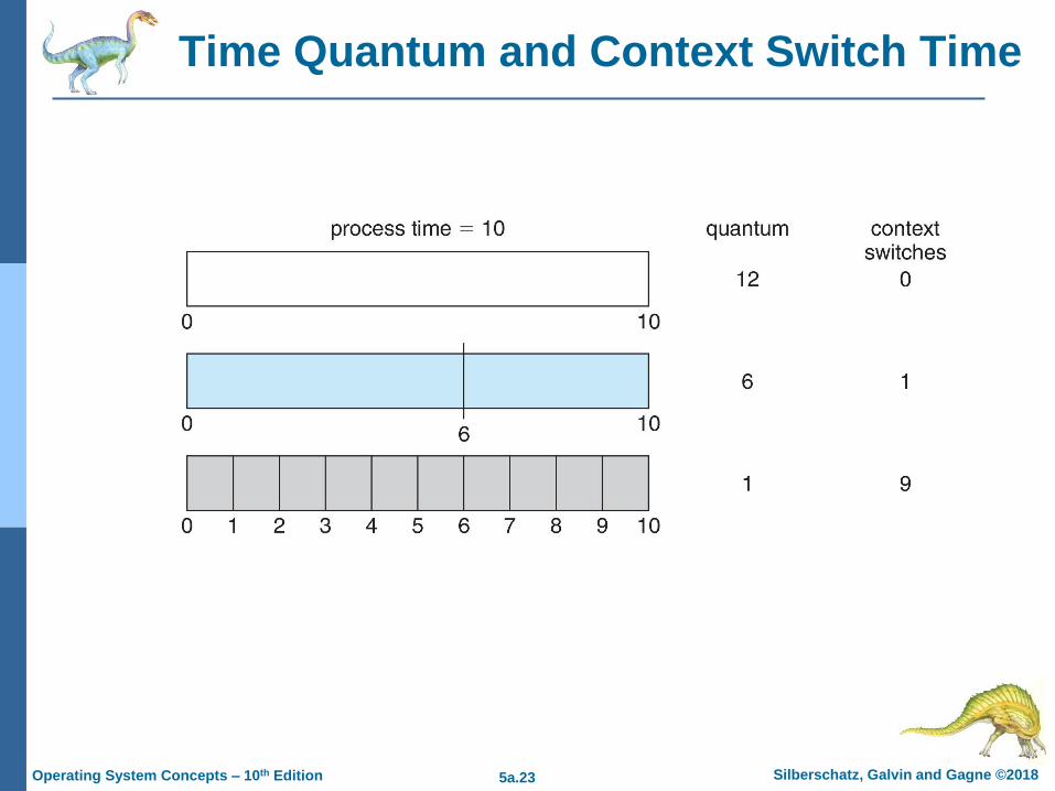
Round Robin (RR)

Each process gets a small unit of CPU time (time quantum q),

usually 10-100 milliseconds. After this time has elapsed, the

process is preempted and added to the end of the ready queue.

If there are n processes in the ready queue and the time quantum

is q, then each process gets 1/n of the CPU time in chunks of at

most q time units at once. No process waits more than (n-1)q

time units.

Timer interrupts every quantum to schedule next process

Performance

• q large FIFO

• q small q must be large with respect to context switch,

otherwise overhead is too high


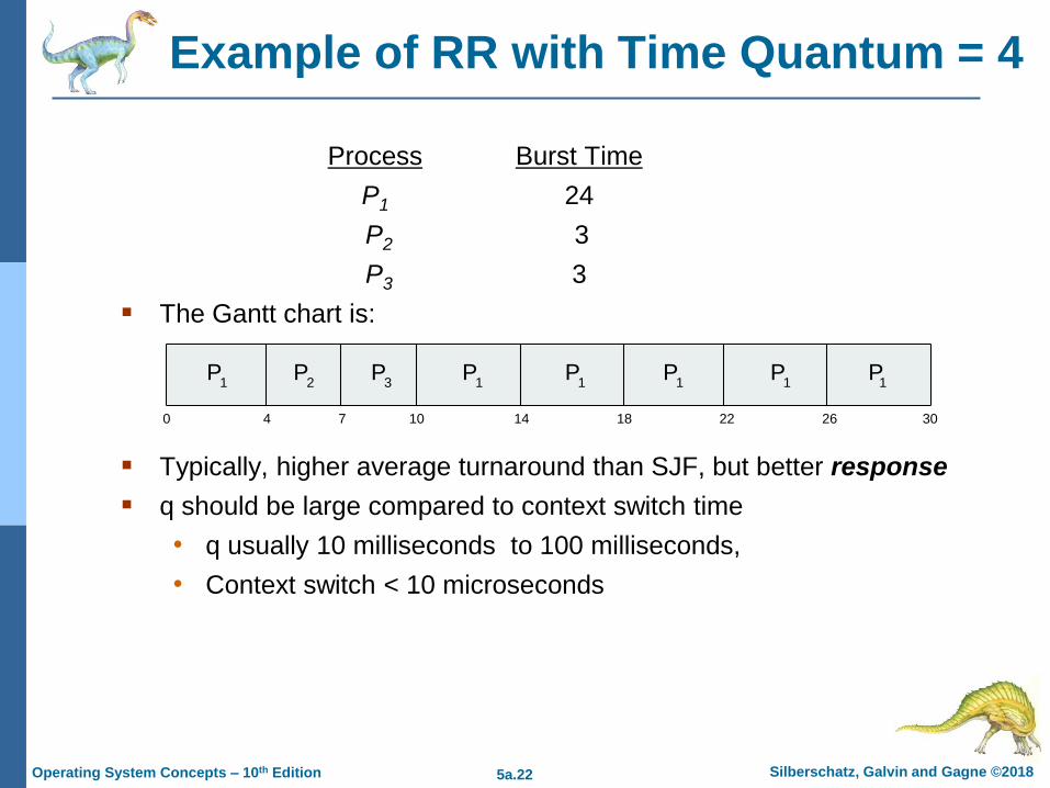
Example of RR with Time Quantum = 4

Process Burst Time

P1 24

P2 3

P3 3

The Gantt chart is:

Typically, higher average turnaround than SJF, but better response

q should be large compared to context switch time

• q usually 10 milliseconds to 100 milliseconds,

• Context switch < 10 microseconds

P P P1 1 1

0 18 3026144 7 10 22

P2

P3

P1

P1

P1


Time Quantum and Context Switch Time


Turnaround Time Varies With The Time Quantum

80% of CPU bursts should be shorter than q


Priority Scheduling

A priority number (integer) is associated with each process

The CPU is allocated to the process with the highest priority (smallest

integer highest priority)

• Preemptive

• Nonpreemptive

SJF is priority scheduling where priority is the inverse of predicted next

CPU burst time

Problem Starvation – low priority processes may never execute

Solution Aging – as time progresses increase the priority of the

process


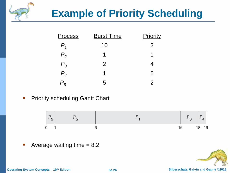
Example of Priority Scheduling

ProcessA arri Burst TimeT Priority

P1 10 3

P2 1 1

P3 2 4

P4 1 5

P5 5 2

Priority scheduling Gantt Chart

Average waiting time = 8.2


Priority Scheduling w/ Round-Robin

ProcessA arri Burst TimeT Priority

P1 4 3

P2 5 2

P3 8 2

P4 7 1

P5 3 3

Run the process with the highest priority. Processes with the same

priority run round-robin

Gantt Chart with time quantum = 2


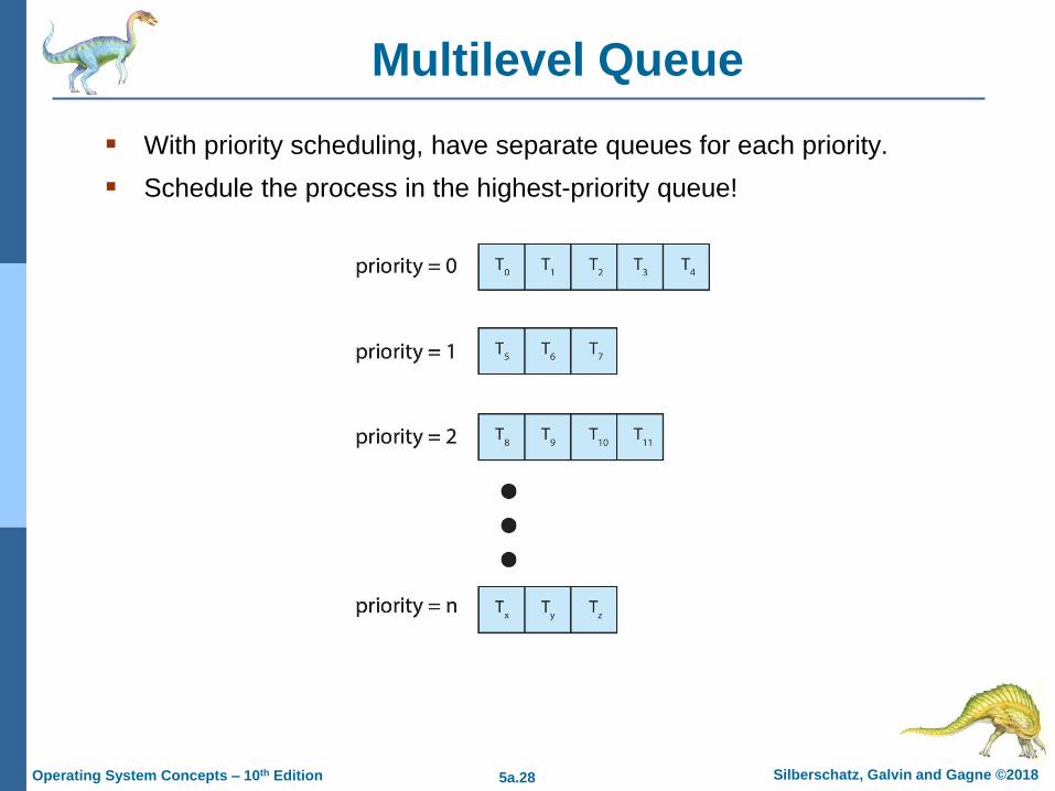
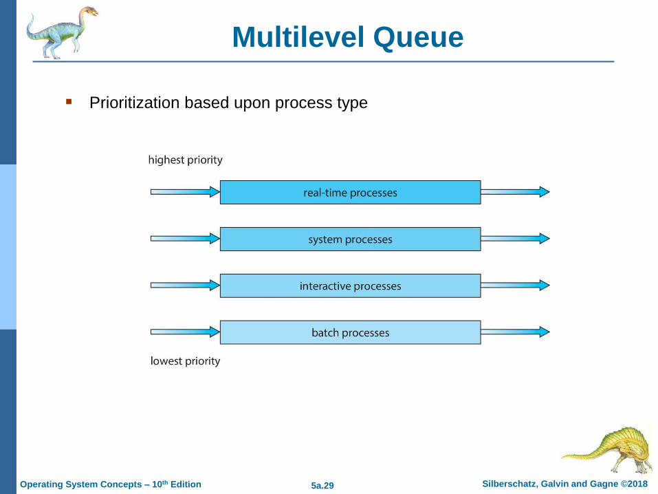
Multilevel Queue

With priority scheduling, have separate queues for each priority.

Schedule the process in the highest-priority queue!


Multilevel Queue

Prioritization based upon process type


Multilevel Feedback Queue

A process can move between the various queues.

Multilevel-feedback-queue scheduler defined by the following

parameters:

• Number of queues

• Scheduling algorithms for each queue

• Method used to determine when to upgrade a process

• Method used to determine when to demote a process

• Method used to determine which queue a process will enter

when that process needs service

Aging can be implemented using multilevel feedback queue


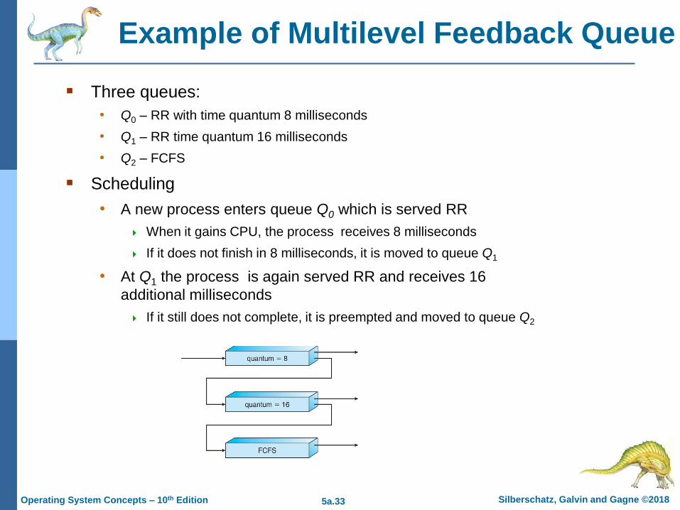
Example of Multilevel Feedback Queue

Three queues:

• Q0 – RR with time quantum 8 milliseconds

• Q1 – RR time quantum 16 milliseconds

• Q2 – FCFS

Scheduling

• A new process enters queue Q0 which is

served in RR

When it gains CPU, the process receives 8

milliseconds

If it does not finish in 8 milliseconds, the

process is moved to queue Q1

• At Q1 job is again served in RR and

receives 16 additional milliseconds

If it still does not complete, it is preempted

and moved to queue Q2


Example of Multilevel Feedback Queue

Three queues:

• Q0 – RR with time quantum 8 milliseconds

• Q1 – RR time quantum 16 milliseconds

• Q2 – FCFS

Scheduling

• A new process enters queue Q0 which is served RR

When it gains CPU, the process receives 8 milliseconds

If it does not finish in 8 milliseconds, it is moved to queue Q1

• At Q1 the process is again served RR and receives 16

additional milliseconds

If it still does not complete, it is preempted and moved to queue Q2

Chapter 5a: CPU Scheduling

Documents

Transcript of Chapter 5a: CPU Scheduling