CHAPTER-5 WAVEPACKETS and THE HEISENBERG UNCERTAINTY PRINCIPLE · CHAPTER-5 WAVEPACKETS and THE...
60
1 Lecture Notes PH 411/511 ECE 598 A. La Rosa INTRODUCTION TO QUANTUM MECHANICS ________________________________________________________________________ CHAPTER-5 WAVEPACKETS and THE HEISENBERG UNCERTAINTY PRINCIPLE Fourier Spectral Decomposition of the Wave-function Understanding of the Heisenberg Uncertainty Principle (as a universal properties of waves) Describing the wavefunction of a free-particle (relativistic and non-relativistic cases) in the context of the wave- particle duality 5.1 Spectral Decomposition of a function (relative to a basis-set) 5.1.A Analogy between the components of a vector V and spectral components of a function 5.1.B The scalar product between two periodic functions 5.1.C How to find the spectral components of a function ? 5.1.C.a Case: Periodic Functions. The Series Fourier Theorem 5.1.C.b Case: Non-periodic Functions The Fourier Integral 5.1.D Spectral decomposition in complex variable. The Fourier Transform 5.1.E Correlation between a localized-functions (f ) and its spread-Fourier (spectral) transforms (F) 5.1.F The scalar product in complex variable 5.1.G Notation in Terms of Brackets 5.2 Phase Velocity and Group Velocity 5.2.A Planes 5.2.B Traveling Plane Waves and Phase Velocity Traveling Plane Waves (propagation in one dimension) Traveling Harmonic Waves 5.2.C A Traveling Wavepackage and its Group Velocity Wavepacket composed of two harmonic waves Analytical description Graphical description Phasor method to analyze a wavepacket
Transcript of CHAPTER-5 WAVEPACKETS and THE HEISENBERG UNCERTAINTY PRINCIPLE · CHAPTER-5 WAVEPACKETS and THE...
1
Lecture Notes PH 411/511 ECE 598 A. La Rosa
INTRODUCTION TO QUANTUM MECHANICS ________________________________________________________________________
CHAPTER-5 WAVEPACKETS and THE HEISENBERG UNCERTAINTY PRINCIPLE
Fourier Spectral Decomposition of the Wave-function
Understanding of the Heisenberg Uncertainty Principle (as a universal properties of waves)
Describing the wavefunction of a free-particle (relativistic and non-relativistic cases) in the context of the wave-particle duality
5.1 Spectral Decomposition of a function (relative to a basis-set)
5.1.A Analogy between the components of a vector V and spectral
components of a function
5.1.B The scalar product between two periodic functions
5.1.C How to find the spectral components of a function ?
5.1.C.a Case: Periodic Functions. The Series Fourier Theorem 5.1.C.b Case: Non-periodic Functions
The Fourier Integral
5.1.D Spectral decomposition in complex variable. The Fourier Transform
5.1.E Correlation between a localized-functions (f ) and its spread-Fourier (spectral) transforms (F)
5.1.F The scalar product in complex variable
5.1.G Notation in Terms of Brackets
5.2 Phase Velocity and Group Velocity
5.2.A Planes
5.2.B Traveling Plane Waves and Phase Velocity Traveling Plane Waves (propagation in one dimension) Traveling Harmonic Waves
5.2.C A Traveling Wavepackage and its Group Velocity Wavepacket composed of two harmonic waves
Analytical description Graphical description
Phasor method to analyze a wavepacket
2
Case: Wavepacket composed of two waves Case: A wavepacket composed of several harmonic waves
5.3 DESCRIBING the MOTION of a FREE PARTICLE in the context of the WAVE-PARTICLE DUALITY
5.3.A Trial-1: A wavefunction with a definite momentum
5.3.B Trial-2: A wavepacket as a wavefunction
References: R. Eisberg and R. Resnick, “Quantum Physics,” 2nd Edition, Wiley, 1985. Chapter 3. D. Griffiths, "Introduction to Quantum Mechanics"; 2nd Edition, Pearson Prentice Hall. Chapter 2.

3
CHAPTER-5 WAVEPACKETS and THE HEISENBERG
UNCERTAINTY PRINCIPLE
Objective: The develop the concepts of “group velocity of a wavepacket,” and the “inner product” between functions (cases of real and complex functions) in order to gain a plausible understanding of the Heisenberg Uncertainty Principle. The wavepacket is decomposed in term of its Fourier components. The inner product is expressed in regular as well as in bracket notation. A quantum mechanics description of the free particle for the non-relativistic and relativist cases are obtained.
In an effort to reach a better understanding of the wave-particle duality1, the motion of a free-particle will be described by a wave packet
x,tcomposed of traveling harmonic waves,
x,t ][)( )( k
tkkxkA Sin
A wavepacket is a function whose values, at a given time, are different from zero only inside a limited
spatial region of extension ~X. From a quantum
mechanics point of view, if a wavepacket of width X is used to represent a particle, X is then interpreted as the region where the particle is likely to be located; that is, there
is an uncertainty about its “exact” location. There will be also an uncertainty P about
the linear momentum of that particle. In this chapter we try to
understand how these two uncertainties, X and P, do relate to each other. Of course, we know those uncertainties are related
through the quantum Heisenberg Principle, but we plan to provide some arguments of why such quantum principle should follow.
STRATEGY:
First, we summarize some general properties of waves and use the Fourier’s spectral decomposition technique as the analytical tool to describe
wavepackets.
Then, when the De Broglie‘s principle of wave-particle duality is
integrated into this description, the interrelation between the spatial and momentum
Spatially localized pulse
x
(x)
X
Fig.1 Accelerometer for automotive
applications.
4
uncertainties, the Heisenberg Principle, will fit in a very logical and consistent way.
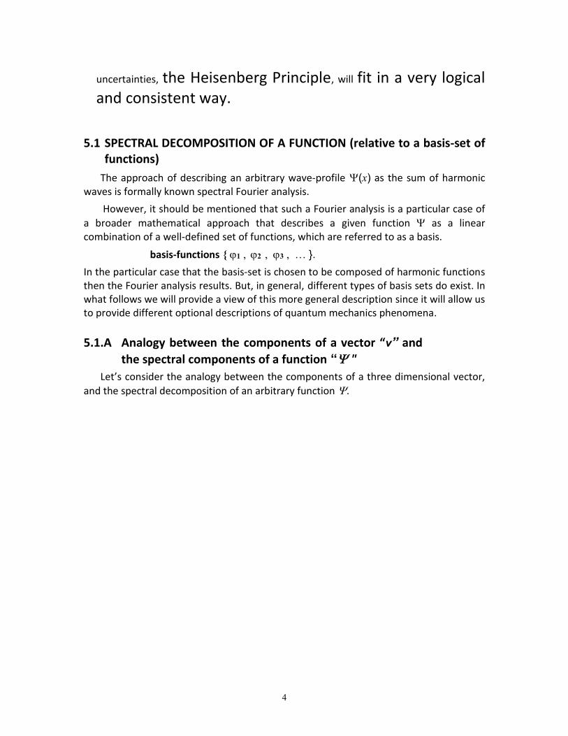
5.1 SPECTRAL DECOMPOSITION OF A FUNCTION (relative to a basis-set of functions)
The approach of describing an arbitrary wave-profile (x) as the sum of harmonic waves is formally known spectral Fourier analysis.
However, it should be mentioned that such a Fourier analysis is a particular case of
a broader mathematical approach that describes a given function as a linear combination of a well-defined set of functions, which are referred to as a basis.
basis-functions { 1 , 2 , 3 , … }.
In the particular case that the basis-set is chosen to be composed of harmonic functions then the Fourier analysis results. But, in general, different types of basis sets do exist. In what follows we will provide a view of this more general description since it will allow us to provide different optional descriptions of quantum mechanics phenomena.
5.1.A Analogy between the components of a vector “v” and
the spectral components of a function “"
Let’s consider the analogy between the components of a three dimensional vector,
and the spectral decomposition of an arbitrary function .

5
Vector v
Function
v = v1 ê1 + v2 ê2 + v3 ê3
= c1 1 + c2 2 + …
Spectral components
Vector components
(1)
The latter means
x = c1 1x + c2 2x + …
where { ê1 , ê2 , ê3} is a particular basis-set
where { 1, 2 , } is a particular basis-set of functions
Vector components In the expression (1) above,
{ê1 , ê2 , ê3 } (2)
is a set of unit vectors perpendicular to each other; that is,
êi êj = ij (3)
ê2
ê1
ê3
v
where ij ≡ 0 if j ≠ i
≡ 1 if j = i
Here A B means “scalar product between vector A and vector B.
How to find the components of a vector v ?
If, for example a vector v were expressed as

6
v = 3 ê1 + 7 ê2 - 2 ê3, then, its component would be given by
ê1 v = 3 ; ê2 v = 7 ; and ê3 v = -2
In a more general case,
if v = v1 ê1 + v2 ê2 + v3 ê3 its components vj are obtained by evaluating the corresponding scalar products
vj = êj v ; for j=1, 2,3
Thus, a vector v can be expressed in terms of the unit vectors in a compact form,
v =
3
1j
(êj v) êj (4)
Notice the involvement of the scalar product to obtain the components of a vector. To the effect of describing the spectral components of a function, we similarly introduce in the following section a type of scalar product between functions.
5.1.B The scalar product between two periodic functions
Set of base functions. In the expression (1) above, we assume that
{ 1 , 2 , 3 , … } (5)
is a infinite basis-set of given functions “perpendicular” to each other.
That is, they fulfill the following relation,
i j = ij
But what would the symbol mean?
To answer this question, we will introduce a definition. Let’s consider first the
particular case where all the functions under consideration are periodic and
real. Let be the periodicity of the functions; that is,
(x + ) = (x) Periodic function (6)
Definition. A scalar product between two periodic (but otherwise
arbitrary) real functions and is defined as follows,
7
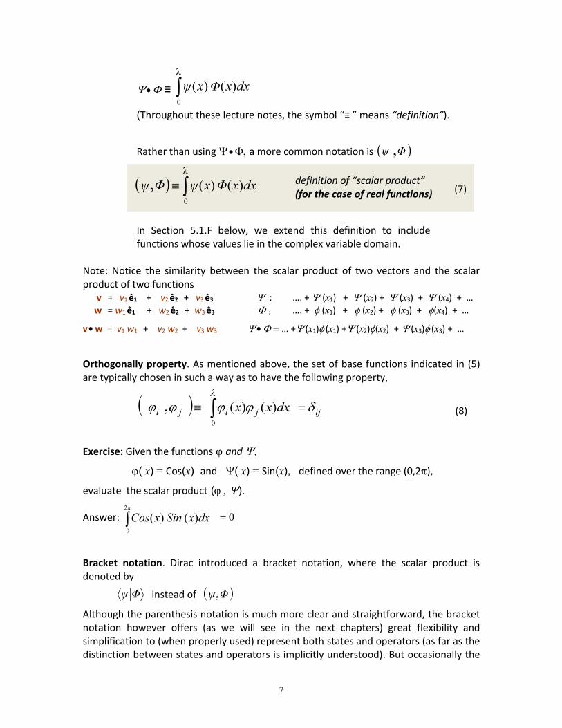
≡
0
)( )( dxxΦxψ
(Throughout these lecture notes, the symbol “≡ ” means “definition”).
Rather than using a more common notation is ,Φψ
0
)( )(, dxxΦxψΦψ (7)
definition of “scalar product” (for the case of real functions)
In Section 5.1.F below, we extend this definition to include functions whose values lie in the complex variable domain.
Note: Notice the similarity between the scalar product of two vectors and the scalar product of two functions v = v1 ê1 + v2 ê2 + v3 ê3 : …. + (x1) + (x2) + (x3) + (x4) + …
w = w1 ê1 + w2 ê2 + w3 ê3 : …. + (x1) + (x2) + (x3) + (x4) + …
v w = v1 w1 + v2 w2 + v3 w3 … +(x1) (x1) +(x2)(x2) +(x3)(x3) + …
Orthogonally property. As mentioned above, the set of base functions indicated in (5) are typically chosen in such a way as to have the following property,
ijjiji dxxx
0
)()(, (8)
Exercise: Given the functions and,
( x) = Cos(x) and ( x) = Sin(x), defined over the range (0,2),
evaluate the scalar product ().
Answer: 2
0
)( )( dxxSinxCos 0
Bracket notation. Dirac introduced a bracket notation, where the scalar product is denoted by
Φψ instead of , Φψ
Although the parenthesis notation is much more clear and straightforward, the bracket notation however offers (as we will see in the next chapters) great flexibility and simplification to (when properly used) represent both states and operators (as far as the distinction between states and operators is implicitly understood). But occasionally the
8
bracket notation will present also difficulties on how to use it. When such cases arise, we will resort back to the parenthesis notation for clarification. Since the bracket notation is so broad spread in quantum mechanics literature, we will frequently use it in this course.
5.1.C How to find the spectral components of a function ?
Given an arbitrary periodic function we wish to express it as a linear combination
of a given base of orthogonal periodic functions { j j
= c1 1 + c2 2 + … (9)
Using the scalar product definition given in (9) we can obtain the corresponding values
of the coefficients cj, in the following manner (adopting the bracket notation for the scalar product),
cj
0
)( dxψ(x x)ψ jj for j= 1,2,3, … (10)
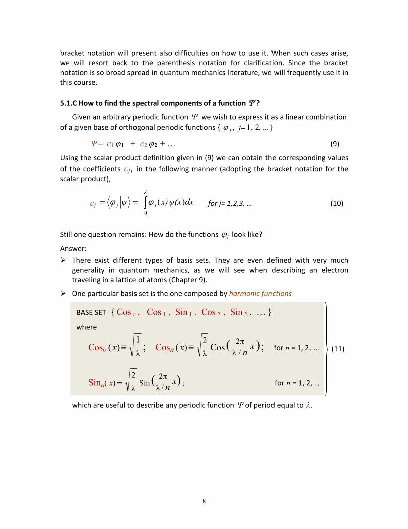
Still one question remains: How do the functions j look like?
Answer:
There exist different types of basis sets. They are even defined with very much generality in quantum mechanics, as we will see when describing an electron traveling in a lattice of atoms (Chapter 9).
One particular basis set is the one composed by harmonic functions
BASE SET { Cos o , Cos 1 , Sin 1 , Cos 2 , Sin 2 , … }
where
Cosoxλ
1 Cosn x
λ
2Cos )(
/
2 x
n
for n = 1, 2, ...
Sinnxλ
2Sin )(
/λ
2x
n
forn = 1, 2, ..
(11)
which are useful to describe any periodic function of period equal to .

9
x
Sin 1
Sin 2
Sin 3
Sin 4
Cos 1
Cos 2
Cos 3
Cos 4
x
Fig. 5.1 Set of harmonic functions defined in expression (11) (shifted up for convenient illustration purposes). They are used as a base to express any periodic
function of periodicity equal to .
It can be directly verified, using the definition of scalar product given in (10), that the harmonic functions defined in (11) satisfy,
Cosn│Sinm =
0
)( )( dxxSinxCos mn 0
More generally,
Cos n│Sinm 0 for arbitrary integers m , n;
Cos n │Cosm mn
for arbitrary integers m , n;
Sin n │Sinm mn
for arbitrary integers m , n.
(12)
5.1.C.a The Series Fourier Theorem: Spectral decomposition of periodic functions
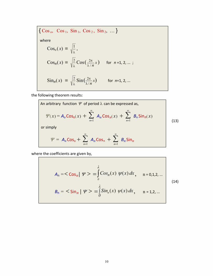
The property (12) leads to the following result:
Using the base-set of harmonic functions of periodicity , defined as follow,
10
{ Cos o, Cos 1, Sin 1, Cos 2 , Sin 2, … }
where
Cosox λ
1,
Cosn x λ
2Cos )(
/
2 x
n
for n =1, 2, ... ;
Sinn x λ
2Sin )(
/λ
2x
n
for n=1, 2, ...
the following theorem results:
An arbitrary function of period can be expressed as,
(x )= Ao Coso(x )
1n
An Cos n(x )
1n
Bn Sin n(x )
or simply
= Ao Coso
1n
An Cos n
1n
Bn Sinn
(13)
where the coefficients are given by,
An= Cos n│ dxx xCos ψλ
0
n )()( n = 0,1,2, ...
Bn = Sin n │ dxxψ xSinλ
0n )()( n = 1,2, ...
(14)

11
1 2 3 4 5 n
An
x
1 2 3 4 5 n
Bn
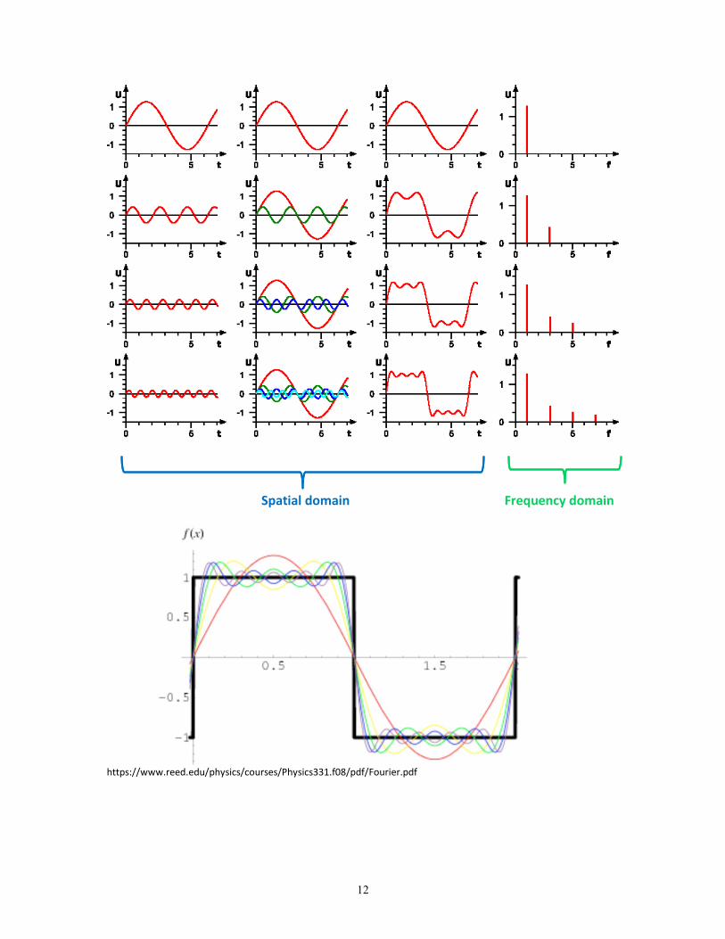
Fig. 5.2 Periodic function and its corresponding Fourier spectrum fingerprint.
Example Fourier approach to reconstruct a function. https://www.google.com/imgres?imgurl=https://cdn.britannica.com/700x450/77/61777-004-EB9FB008.jpg&imgrefurl=https://www.britannica.com/science/Fourier-analysis&h=336&w=405&tbnid=NeKr_PRelMD_gM:&q=fourier+decomposition&tbnh=124&tbnw=150&usg=AI4_-kTUhxMn1_ww00uN6cMx0zyhn4CcCg&vet=12ahUKEwiFw4Tu3O3dAhXkz4MKHU0JABgQ_B0wFHoECAYQEw..i&docid=kZqBYHox5aKOaM&itg=1&sa=X&ved=2ahUKEwiFw4Tu3O3dAhXkz4MKHU0JABgQ_B0wFHoECAYQEw#h=336&imgdii=PVL2zqJ8xb2tXM:&tbnh=124&tbnw=150&vet=12ahUKEwiFw4Tu3O3dAhXkz4MKHU0JABgQ_B0wFHoECAYQEw..i&w=405
12
Spatial domain Frequency domain
https://www.reed.edu/physics/courses/Physics331.f08/pdf/Fourier.pdf
13
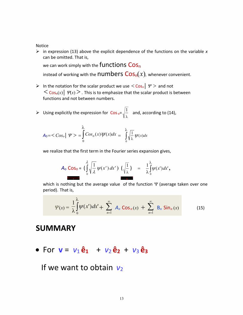
Notice in expression (13) above the explicit dependence of the functions on the variable x
can be omitted. That is,
we can work simply with the functions Cosn
instead of working with the numbers Cosnx whenever convenient.
In the notation for the scalar product we use Cosn│ and not
Cosn(x)│(x) . This is to emphasize that the scalar product is between functions and not between numbers.
Using explicitly the expression for Cos o=λ
1 and, according to (14),
A0 Coso│ dxxxCos ψ )( )(
0
o
dxxψ )( 1
0
we realize that the first term in the Fourier series expansion gives,
Ao Coso = ( dx'x'ψ )( 1
0
(
λ
1) ')'(
λ
1
0
dxxψ
which is nothing but the average value of the function (average taken over one period). That is,
x= ')'(λ
1
0
dxxψ
1n
An Cos n x
1n
Bn Sin nx (15)
SUMMARY
For v = v1 ê1 + v2 ê2 + v3 ê3
If we want to obtain v2
14
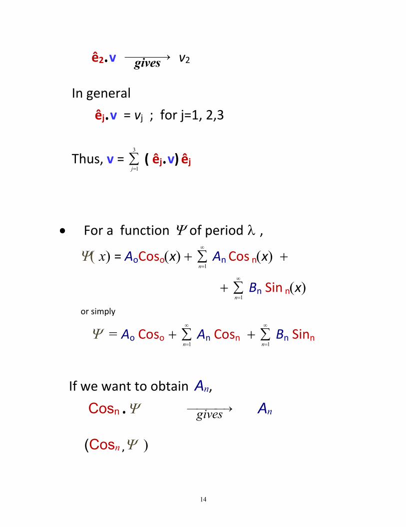
ê2 v gives v2
In general
êj v = vj ; for j=1, 2,3
Thus, v =
3
1j
( êj v) êj
For a function of period ,
x= AoCosox
1n
An Cos nx
1n
Bn Sin nx
or simply
= Ao Coso
1n
An Cosn
1n
Bn Sinn
If we want to obtain An,
Cosn gives An
(Cosn ,

15
Cosn │
dxxxCos ψ )( )(
0
n
Just different notations for the same quantity
Spatial frequency k
of the corresponding
harmonic function
Cosoxλ
1 ,
Cos1 xλ
2Cos )(
1/
2 x
k
2
Cos2 xλ
2Cos )(
2/
2 x
k
2
Cos3 xλ
2Cos )(
3/
2 x
k
2

16
5.1.C.b Spectral decomposition of Non-periodic
Functions: The Fourier Integral The series Fourier expansion allows the analysis of periodic functions, where
specifies the periodicity. For the case of non-periodic functions a similar analysis is pursued by taking the limit when .
For an arbitrary function of period we have the Fourier series expansion,
x= Ao Cos ox
1n
An Cos nx
1n
Bn Sin nx
Writing the base-functions in a more explicit form (using expression (11)), one obtains,
x=
1
0
)( dxx
1 nAn
2Cos )(
n/
2x
1 nBn
2Sin )(
n/
2x
Cos n(x) Sin n(x)
Since and all the harmonic functions have period , we can change the
interval of interest (0, ) to (-/ 2, / 2) instead, and thus re-
write,

17
x=
1
2/
2/
')'( dxxψ
1 n
An [ )n2
( x
Cos
2 ]
1 n
Bn [ )n2
( x
Sin
2 ]
whereAn Cos n │
2/
2/
[ )'n 2
( x
Cos
2 ] dx'x'ψ )( n=1,2, ...
Bn Sin n│
2/
2/
[ )'n 2
( x
Sin
2 ] dx'x'ψ )( ;n= 1,2, ...
Cos n(x) Sin n(x)
(15)’
Let’s define
2ok and on nkk (16)
Notice, when , the quantity
2ok becomes
infinitesimally small
Using (16), expression (15)’ adopts the form,
x=
1
2/
2/
')'( dxxψ
1 n
An [ )( x0kn Cos 2
]
1 n
Bn [ ) ( x0kn Sin2
] (15)”
18
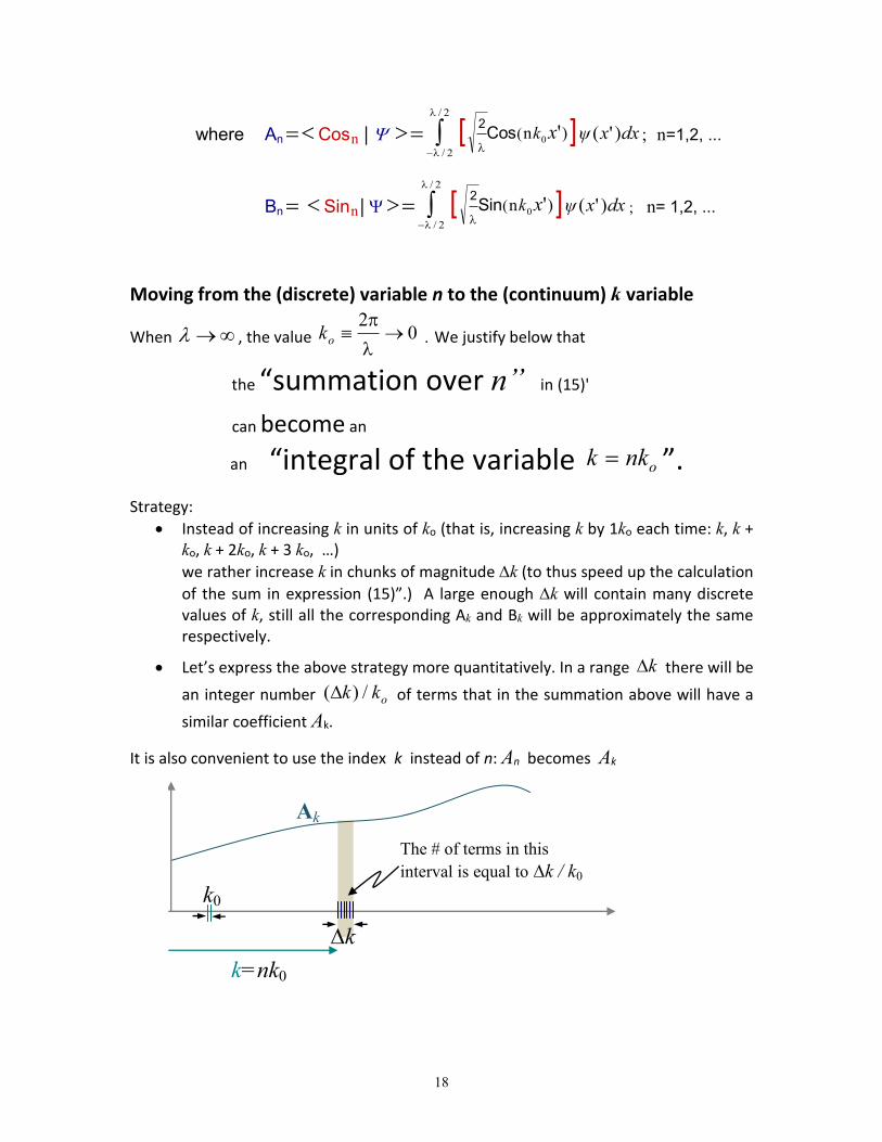
where An Cos n │
2/
2/
[ )n '0 ( xkCos2
] dxxψ )'( n=1,2, ...
Bn Sin n│
2/
2/
[ )n '0 ( xkSin2
] dxxψ )'( ;n= 1,2, ...
Moving from the (discrete) variable n to the (continuum) k variable
When , the value 02
ok We justify below that
the “summation over n” in (15)'
can become an
an “integral of the variable onkk ”.
Strategy:
Instead of increasing k in units of ko (that is, increasing k by 1ko each time: k, k + ko, k + 2ko, k + 3 ko, …)
we rather increase k in chunks of magnitude k (to thus speed up the calculation
of the sum in expression (15)”.) A large enough k will contain many discrete values of k, still all the corresponding Ak and Bk will be approximately the same respectively.
Let’s express the above strategy more quantitatively. In a range k there will be
an integer number okk /)( of terms that in the summation above will have a
similar coefficient Ak.
It is also convenient to use the index k instead of n: An becomes Ak
k0
k=nk0
Ak
k
The # of terms in this
interval is equal to k / k0
19
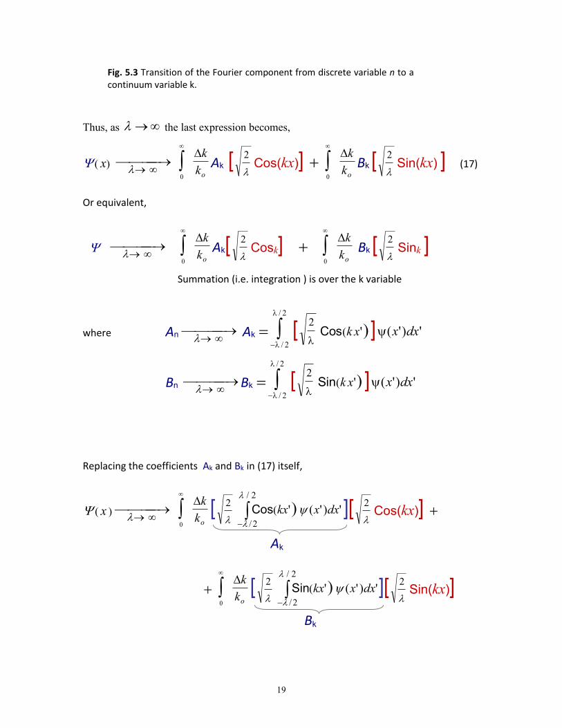
Fig. 5.3 Transition of the Fourier component from discrete variable n to a continuum variable k.
Thus, as the last expression becomes,
x
0 ok
kAk [
2Cos(kx)]
0 ok
kBk [
2Sin(kx)] (17)
Or equivalent,
0 ok
kAk[
2Cosk]
0 ok
k Bk [
2Sink]
Summation (i.e. integration ) is over the k variable
where An
Ak
2/
2/
[
2)' ( xkCos ] ')'( dxx
Bn
Bk
2/
2/
[
2)' ( xkSin ] ')'( dxx
Replacing the coefficients Ak and Bkin (17) itself,
( x )
0 ok
k [
2')'('
2/
2/
)( dxxkx
Cos ][
2Cos(kx)]
0 ok
k [
2')'('
2/
2/
)( dxxkx
Sin ][
2Sin(kx)]
Ak
Bk
20
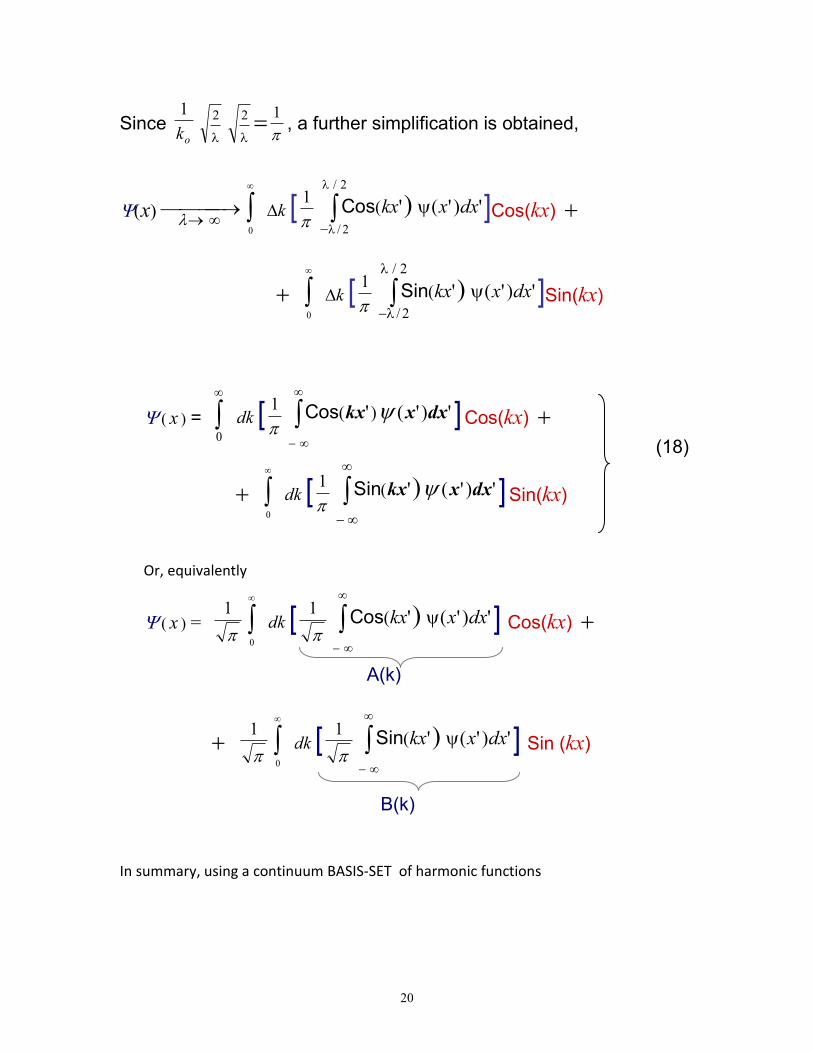
Since ok
1
2
2
1, a further simplification is obtained,
x
0
k [
1')'('
2/
2/
)( dxxkx
Cos ]Cos(kx)
0
k [
1')'('
2/
2/
)( dxxkx
Sin ]Sin(kx)
( x )=
0
dk [
1 ')'(' )( dxxkx
Cos ] Cos(kx)
0
dk [
1 ')'(')( dxxkx
Sin ] Sin(kx)
(18)
Or, equivalently
( x )=
1
0
dk [
1')'(')( dxxkx
Cos ] Cos(kx)
1
0
dk [
1')'(')( dxxkx
Sin ] Sin (kx)
A(k)
B(k)
In summary, using a continuum BASIS-SET of harmonic functions

21
{ Cosk , Sink ; k0 } (19)
where
Cos k( x) Cos(kx) and Sink( x) Sin(kx)
we have demonstrated that an arbitrary function (x) can be expressed as a linear combination of such basis-set functions,
( x ) =
1
0
A(k) Cosk(x) dk
1
0
B(k) Sink(x) dk
where the amplitude coefficients of the harmonic functions components are given by,
A(k) =
1
dx'kx'x' )(Cos )( , and
B(k) =
1
dx'kx'x' )(Sin )(
Fourier coefficients
(20)
22
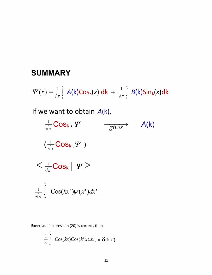
SUMMARY
(x) =
1
0
A(k)Cosk(x) dk
1
0
B(k)Sink(x)dk
If we want to obtain A(k),
1Cosk
gives A(k)
(
1Cosk ,
1Cosk │
1
')'()'(Cos dxxkx ,
Exercise. If expression (20) is correct, then
1
dxxk'kx )(Cos)(Cos , = (k-k’)

23
where is the Delta Dirac
Answer:
Multiplying expression (20) by
1)(Cos xk' on both sides of the equality, and then
integrating from x= - ∞ to x= ∞, we obtain,
24
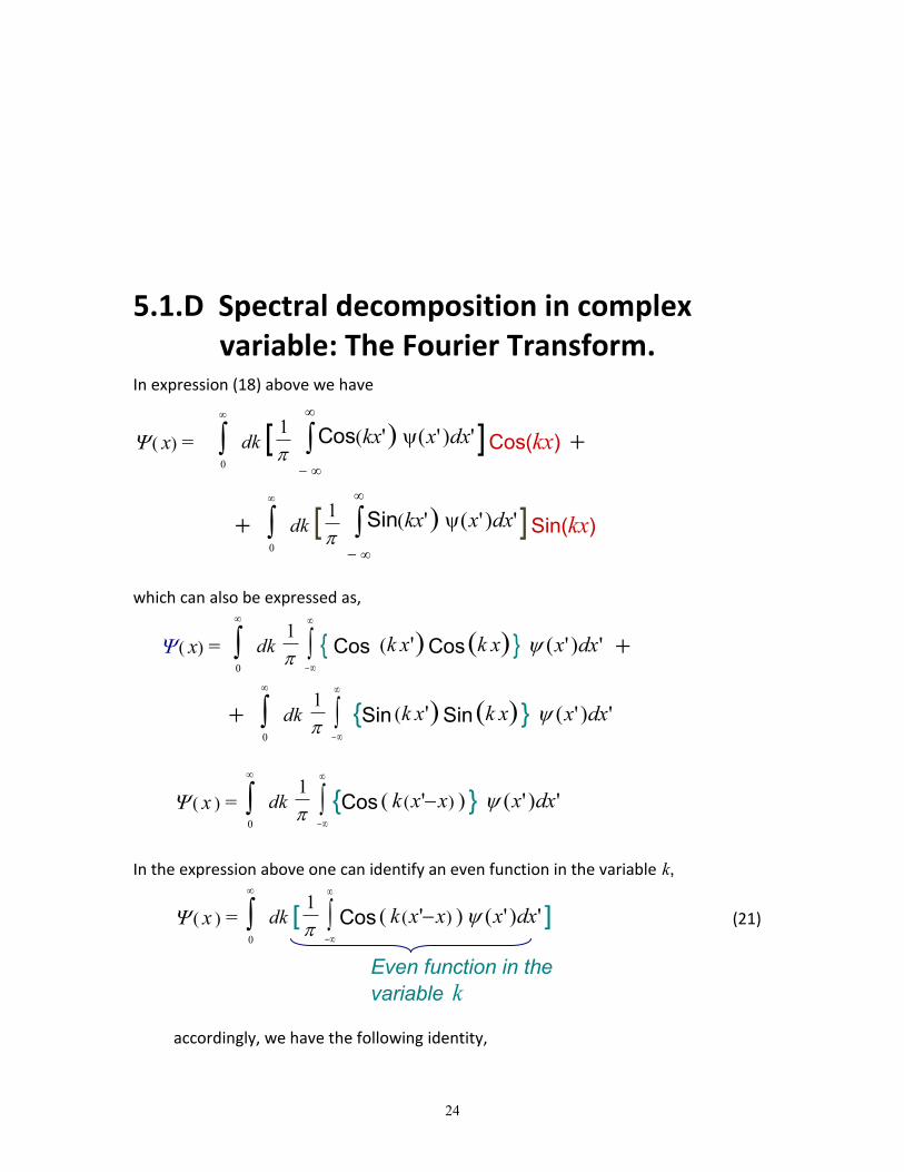
5.1.D Spectral decomposition in complex variable: The Fourier Transform.
In expression (18) above we have
x=
0
dk [
1')'(')( dxxkx
Cos ] Cos(kx)
0
dk [
1')'(')( dxxkx
Sin ] Sin(kx)
which can also be expressed as,
x=
0
dk
1
{ Cos )' ( xk Cos )( xk } ')'( dxx
0
dk
1
{Sin )' ( xk Sin )( xk } ')'( dxx
( x )=
0
dk
1
{Cos ) ' ( )( xxk } ')'( dxx
In the expression above one can identify an even function in the variable k,
( x )=
0
dk [
1
Cos ) ' ( )( xxk ')'( dxx ](21)
Even function in the
variable k
accordingly, we have the following identity,
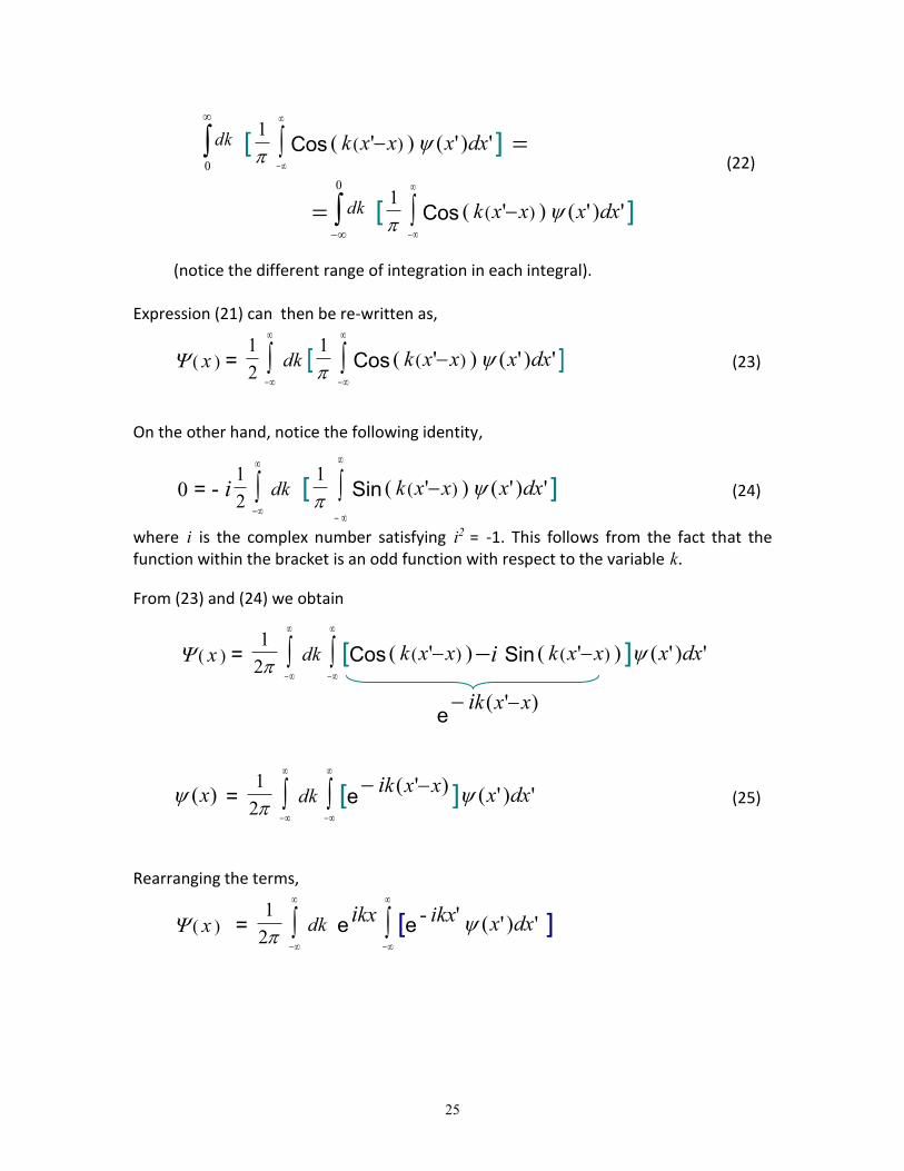
25
0
dk [
1
Cos ) ' ( )( xxk ')'( dxx ]
0
dk [
1
Cos ) ' ( )( xxk ')'( dxx ]
(22)
(notice the different range of integration in each integral).
Expression (21) can then be re-written as,
( x )= 2
1
dk [
1
Cos ) ' ( )( xxk ')'( dxx ] (23)
On the other hand, notice the following identity,
= - i2
1
dk [
1
Sin ) ' ( )( xxk ')'( dxx ] (24)
where i is the complex number satisfying i2 = -1. This follows from the fact that the function within the bracket is an odd function with respect to the variable k.
From (23) and (24) we obtain
( x )= 2
1
dk
[Cos ) ' ( )( xxk i Sin ) ' ( )( xxk ] ')'( dxx
e)'( xxki
)(x = 2
1
dk
[e )'( xxki ] ')'( dxx (25)
Rearranging the terms,
( x )= 2
1
dk ekxi
[e '- ikx ')'( dxx ]
26
( x )= 2
1
2
1
[e'- ikx
dx'x' )( ]exk i
dk
F(k)
( x )=
2
1
F(k)exk i
dk
where F(k) = 2
1
e'- ikx dx'x' )(
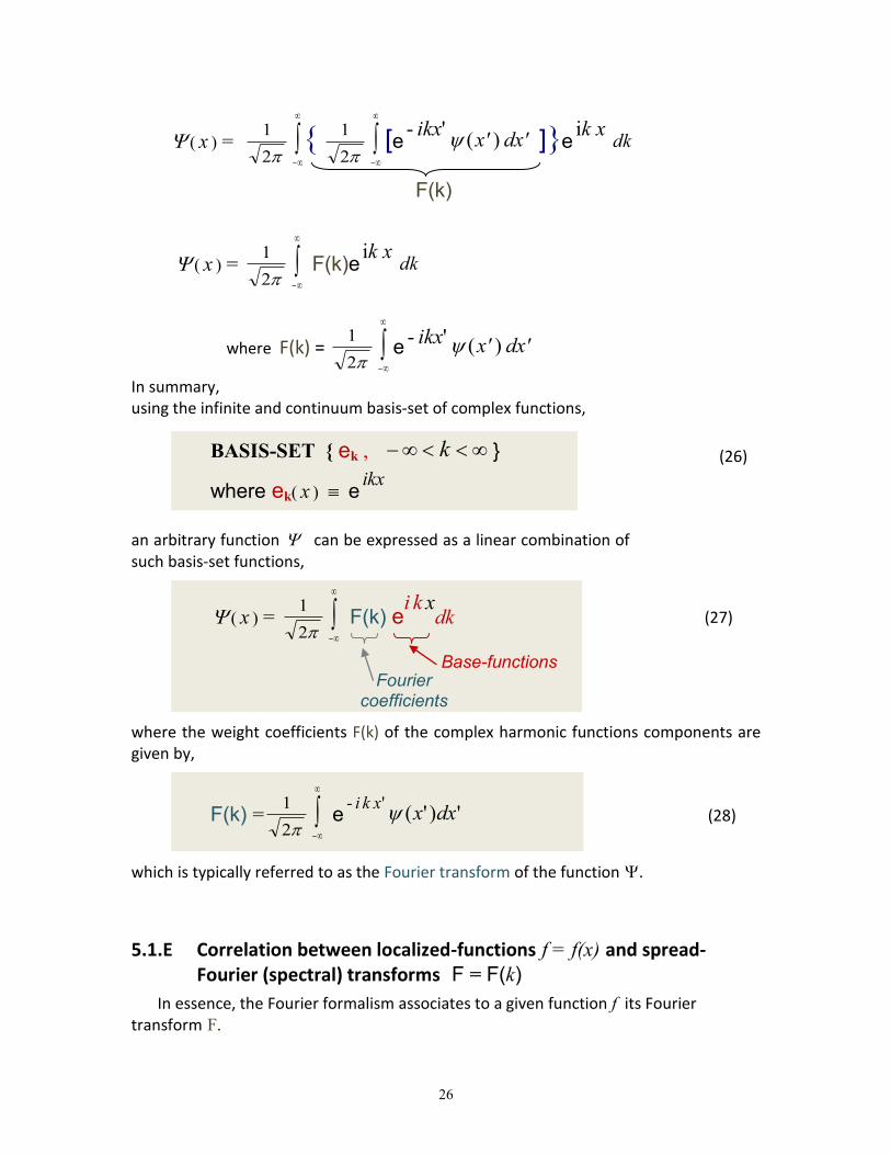
In summary, using the infinite and continuum basis-set of complex functions,
BASIS-SET { ek , k }
where ek( x ) eikx
(26)
an arbitrary function can be expressed as a linear combination of such basis-set functions,
( x )= 2
1
F(k) ei
k
xdk
Fourier coefficients
(27)
Base-functions
where the weight coefficients F(k) of the complex harmonic functions components are given by,
F(k) =2
1
e' - xki
')'( dxx (28)
which is typically referred to as the Fourier transform of the function .
5.1.E Correlation between localized-functions f = f(x) and spread-
Fourier (spectral) transforms F = F(k)
In essence, the Fourier formalism associates to a given function f its Fourier transform F.

27
F f
An important characteristic in the Fourier formalism is that, it turns out,
the more localized is the function f, the broader its spectral Fourier transform F(k); and vice versa.
(29)
Spatially corresponding Fourier localized pulse spatial spectra
Wider pulse narrower Fourier spectra
x
f (x)
g (x)
k
k
F (k)
G(k)
x
Fig. 5.4 Reciprocity between a function and its spectral Fourier transform.
Due to its important implication in quantum mechanics, this
property (29) will be described in greater detail in the Section
5.2 below. It is worth to emphasize here, however, that the property expressed in (29) has nothing to do with quantum mechanics. It is rather an intrinsic property of the Fourier analysis of waves. However, later on when we identify (via the de Broglie hypothesis) some variables in the mathematical Fourier description of waves with corresponding physical variables characterizing a particle (i.e. position, linear momentum, etc), a better understanding of the quantum mechanical description of the world at the atomic level can be obtained.
28
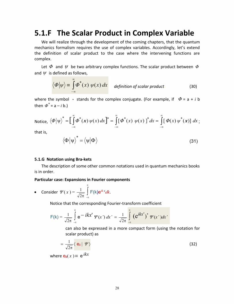
5.1.F The Scalar Product in Complex Variable We will realize through the development of the coming chapters, that the quantum
mechanics formalism requires the use of complex variables. Accordingly, let’s extend the definition of scalar product to the case where the intervening functions are complex.
Let Φ and ψ be two arbitrary complex functions. The scalar product between Φ
and ψ is defined as follows,
dxxψxΦψΦ )()(*definition of scalar product. (30)
where the symbol * stands for the complex conjugate. (For example, if Φ = a + i b
then *Φ = a – i b.)
Notice,
dxψxΦ dxxψxΦdxxψΦΦ )]()([])()([ )()(ψ ****** ][ xx ;
that is,
ψψ*
(31)
5.1.G Notation using Bra-kets
The description of some other common notations used in quantum mechanics books is in order.
Particular case: Expansions in Fourier components
Consider ( x )= 2
1
F(k)eik xdk.
Notice that the corresponding Fourier-transform coefficient
F(k) = 2
1
e 'ikx (x’ ) dx’2
1
*)'(eikx(x’ )dx’
can also be expressed in a more compact form (using the notation for scalar product) as
2
1 ek (32)
whereek( x ) e ikx
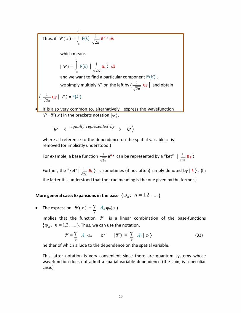
29
Thus, if ( x )=
F(k) 2
1eik x dk
which means
=
F(k) 2
1ek dk
and we want to find a particular component F(k’) ,
we simply multiply on the left by 2
1 ek’ and obtain
2
1ek’ = F(k’)
It is also very common to, alternatively, express the wavefunction
( x ) in the brackets notation ψ
bydrepresenteequally
where all reference to the dependence on the spatial variable x is removed (or implicitly understood.)
For example, a base function 2
1eik x can be represented by a “ket”
2
1 e k .
Further, the “ket” 2
1 ek is sometimes (if not often) simply denoted by k . (In
the latter it is understood that the true meaning is the one given by the former.)
More general case: Expansions in the base { , ...,nn 21; }.
The expression ( x ) = n
An n( x )
implies that the function is a linear combination of the base-functions
{ , ...,nn 21; }. Thus, we can use the notation,
= n
An n or = n
An n (33)
neither of which allude to the dependence on the spatial variable.
This latter notation is very convenient since there are quantum systems whose wavefunction does not admit a spatial variable dependence (the spin, is a peculiar case.)
30
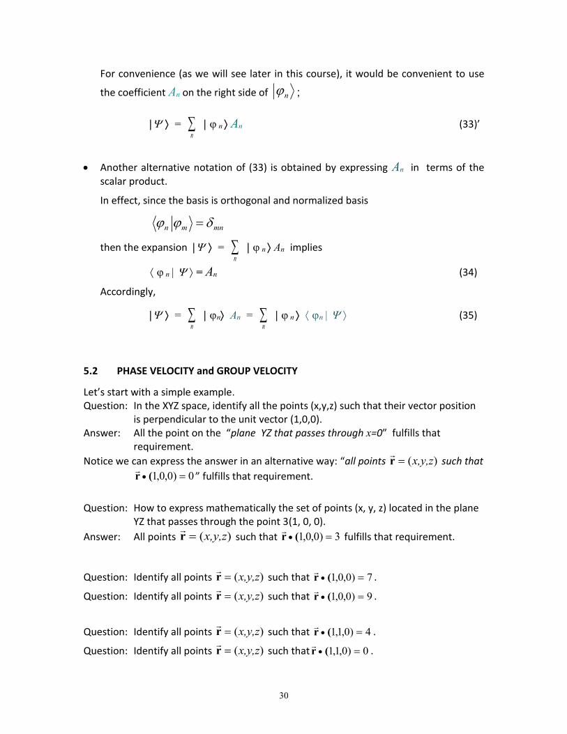
For convenience (as we will see later in this course), it would be convenient to use
the coefficient An on the right side of n ;
= n
n An (33)’
Another alternative notation of (33) is obtained by expressing An in terms of the scalar product.
In effect, since the basis is orthogonal and normalized basis
mnmn
then the expansion = n
n An implies
n = An (34)
Accordingly,
= n
n An = n
n n (35)
5.2 PHASE VELOCITY and GROUP VELOCITY
Let’s start with a simple example. Question: In the XYZ space, identify all the points (x,y,z) such that their vector position
is perpendicular to the unit vector (1,0,0). Answer: All the point on the “plane YZ that passes through x=0” fulfills that
requirement.
Notice we can express the answer in an alternative way: “all points )(x,y,zr
such that
0)0,0,1 (r
” fulfills that requirement.
Question: How to express mathematically the set of points (x, y, z) located in the plane YZ that passes through the point 3(1, 0, 0).
Answer: All points )(x,y,zr
such that 3)0,0,1 (r
fulfills that requirement.
Question: Identify all points )(x,y,zr
such that 7)0,0,1 (r
.
Question: Identify all points )(x,y,zr
such that 9)0,0,1 (r
.
Question: Identify all points )(x,y,zr
such that 4)0,1,1 (r
.
Question: Identify all points )(x,y,zr
such that 0)0,1,1 (r
.
31
Question: Identify all points )(x,y,zr
such that 4)0,1,1 (r
.
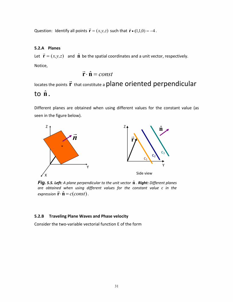
5.2.A Planes
Let )(x,y,zr
and n̂ be the spatial coordinates and a unit vector, respectively.
Notice,
constnr ˆ
locates the points r
that constitute a plane oriented perpendicular
to n̂ .
Different planes are obtained when using different values for the constant value (as
seen in the figure below).
r
X
Y
Z
n
Y
Z
r
c1 c2
c3
n̂
Side view
Fig. 5.5. Left: A plane perpendicular to the unit vector n̂ . Right: Different planes are obtained when using different values for the constant value c in the
expression )(ˆ constcnr
.
5.2.B Traveling Plane Waves and Phase velocity
Consider the two-variable vectorial function E of the form

32
)v(),( ˆ tt -rr n
fo
EE
phase
Function
Constant vector
where f is an arbitrary one-variable function and o
E
is a constant vector.
For example, f could be the Cos function; i.e.
)v(),( ˆcos tt -rr n
oEE )
Notice, the points over a plane oriented perpendicular to n̂ and traveling with velocity
v define the locus of points where the phase of the wave E
remains constant. For this
reason, the wave )v(),( ˆcos tt -rr n
oEE is called a plane wave.
Z
X Y
n̂
Fig. 5.6 Schematic representation of a plane wave of electric fields. The figure shows the electric fields at two different planes, at a given instant of time. The fields lie oriented on the corresponding planes. The planes
are perpendicular to the unit vector n̂ .
Traveling Plane Waves (propagation in one dimension)
)v( txf For any arbitrary function f , this represents a wave
propagating to the right with speed v.

33
f could be COS, EXP, ... etc.
f ( x – vt )
phase
Notice, a point x advancing at speed v will
keep the phase of the wave f constant.
For this reason v is called the phase velocity
vph.
Traveling Harmonic Waves
])([)( tk
xkCOStkxCOS
and )( txkie
These are specific examples of waves propagating to the right
with phase velocity vph= / k.
In general )(kωω .
Note: The specific relationship )(kωω depends on the specific
physical system under analysis (waves in a crystalline array of atoms, light propagation in a free space, plasmons propagation at a metal-dielectric interface, etc.]
)(kωω implies that, for different values of k, the
corresponding waves travel with different phase velocities.
5.2.C A Traveling Wave-package and its Group Velocity
Consider the expression
dkikxkFx ef
)()2/1()(
as the representation of a pulse profile at t=0. Here ikxe
is the profile of the
harmonic wave )( tkxi
e
at 0t .
The profile of this pulse at a later time will be represented by,
)()(
2
1),(
kFedktx
txkiψ
Pulse composed by a group of traveling harmonic waves
(36)
Since, each component )( tkxie
of the group travels with its own phase velocity,

34
would still be possible to associate a unique velocity to the propagating group of waves?
The answer is positive; it is called group velocity. Below we present an example that helps to illustrate this concept.
Case A: Wavepacket composed of two harmonic waves Analytical description
For simplicity, let’s consider the case in which the packet of waves consists if only two waves of very similar wavelength and frequencies.
])([][)( Δω)t(ωxΔkkCos tωkxCostx,ψ (37)
Using the identities )()()()()( BSinASinBCosACosBACos and
)( )()( )()( BSinASinBCosACosBACos one obtains
)()(2)()( BCosACosBACosBACos , which can be expressed as
)( )( 2)()(22
BABACosCosBCosACos
Accordingly, (38) can be expressed as,
])()([ ])()([2),(2222
txkCostxCostxkk
Since we are assuming that and kk , we have
][])2
()2
([2),( tkxCostxk
Costx
Modulation envelope
(38)
Notice, the modulation envelope travels with velocity equal to
k
g
v , (39)
which is known as the group velocity.
In summary,

35
][])2
()2
([2),( tkxCostxk
Costx
(40)
Carrier w a v e Amplitude
Modulating wave Plane of constant p h a s e traveling with speed
k
ωp
V
Planes, where the amplitude of the resultant wave remains constant, travel
with speed k
ωgV
The phase velocity is a measure of the velocity of the harmonic waves components that constitute the wave. The group velocity is the velocity with which, in particular, the profiles of maximum interference propagate. More general, the group velocity is the velocity at which the “envelope” profile propagate (as will be observed better in the graphic analysis given below).
Graphical description
EXAMPLE-1: Visualization of the addition of two waves whose k’s and ’s are very similar in value. Case: Waves components of similar phase velocity, and group-velocity
similar to the phase velocities.
Let,
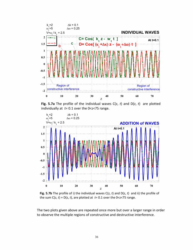
C(z, t) = Cos [k1z –1t] = Cos [ 2 z – t ] (41)
D(z, t) = Cos [k2z –2 t] = Cos [ 2.1 z – t ]
36
Fig. 5.7a The profile of the individual waves C(z, t) and D(z, t) are plotted individually at t= 0.1 over the 0<z<75 range.
Fig. 5.7b The profile of i) the individual waves C(z, t) and D(z, t) and ii) the profile of the sum C(z, t) + D(z, t), are plotted at t= 0.1 over the 0<z<75 range.
The two plots given above are repeated once more but over a larger range in order to observe the multiple regions of constructive and destructive interference.
-2
-1.5
-1
-0.5
0
0.5
1
1.5
2
0 10 20 30 40 50 60 70
At t=0.1C
D
E
z
D= Cos[ (+ z - (
t ]
C= Cos( k1 z - w
1 t ]
DC
Region of
constructive interference
=5 = 0.25
V=/ k
1 = 2.5
k1=2 k = 0.1
Region of
constructive interference
INDIVIDUAL WAVES
-2
-1.5
-1
-0.5
0
0.5
1
1.5
2
0 10 20 30 40 50 60 70
At t=0.1
C
D
E
z
D= Cos[ (+ z - ( t ]
C= Cos( k1 z - w
1 t ]
D
C
Regions of
constructive interference
Regions of
constructive interference
ADDITION of WAVES
=5 = 0.25
V=/ k
1 = 2.5
k1=2 k = 0.1
37
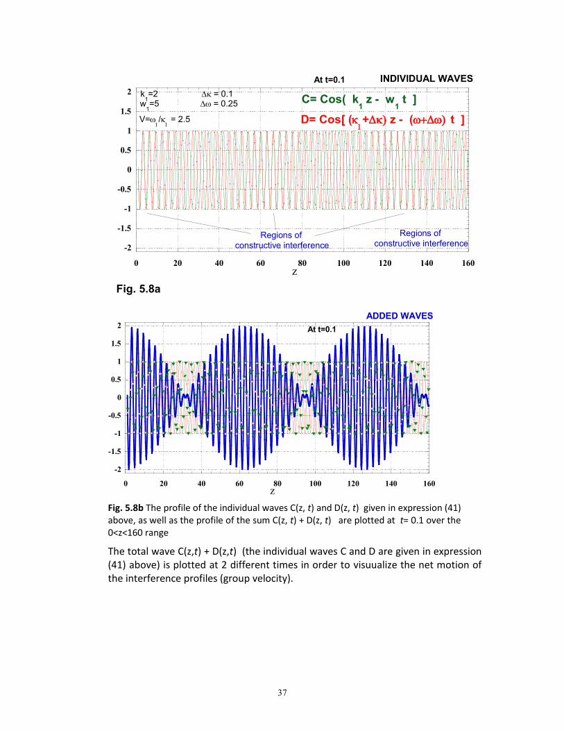
Fig. 5.8a
Fig. 5.8b The profile of the individual waves C(z, t) and D(z, t) given in expression (41) above, as well as the profile of the sum C(z, t) + D(z, t) are plotted at t= 0.1 over the 0<z<160 range
The total wave C(z,t) + D(z,t) (the individual waves C and D are given in expression (41) above) is plotted at 2 different times in order to visuualize the net motion of the interference profiles (group velocity).
-2
-1.5
-1
-0.5
0
0.5
1
1.5
2
0 20 40 60 80 100 120 140 160
At t=0.1
C
D
E
z
D= Cos[ (+ z - ( t ]
C= Cos( k1 z - w
1 t ]
C
Regions of
constructive interference
w1=5 = 0.25
V=/
= 2.5
k1=2 = 0.1
Regions of
constructive interference
INDIVIDUAL WAVES
-2
-1.5
-1
-0.5
0
0.5
1
1.5
2
0 20 40 60 80 100 120 140 160
At t=0.1
C
D
E
z
D= Cos[ (+ z - ( t ]
C= Cos( k1 z - w
1 t ]
D
C
Regions of
constructive interference
w1=5 = 0.25
V=/
= 2.5
Regions of
constructive interference
ADDED WAVES
k1=2

38
-1.2
0
1.2
2.4
20 40 60 80 100
SUM_at_t=0.1_and_t=4_DATA
SUM at t=0.1
SUM at t=4
Cos[ 0.5(Dk)x-0.5(Dw)0.1 ]
Cos[ 0.5(Dk)x-0.5(Dw)4 ]
SU
M a
t t=
0.1
Co
s[ 0
.5(D
k)x
-0.5
(Dw
)0.1
]
z
at t=0.1C+Dat t=4
C= Cos( k1 z - w
1 t ]
D= Cos[ (k1+k) z - (
+t ]
GROUP VELOCITY = 2.5
C+D
=5 = 0.25
Vphase
=/ k
1 = 2.5 V
group=k =2.5
k1=2 k = 0.1
at t=0.1
Envelope
profileat t=4
Envelope
profile
10 x = 10
t = 3.9
Fig. 5.9 Notice, the net displacement of the valley is ~10 units, which occurs during an incremental time of 4 - 0.1 =3.9 units. This indicates that the envelope profile travels with a velocity equal to 10 / 3.9 ~ 2.5. This value coincides with the value of
k = 0.25/01.
In the example above:
The phase velocity of the individual waves are 5/2= 2.5 and 5.25/2.1= 2.5
The group velocity as observed in the graph above is: 10/3.9 = 2.5
The group velocity as calculated from k is 2.5
EXAMPLE-2: Visualization of the addition of two waves whose k’s and ’s are very similar in value. Case: Waves components of similar phase velocity, but group-velocity different
than the phase velocity.
Let,
C(z, t) = Cos [k1z –1t] = Cos [ 2 z – t ] (42)
D(z, t) = Cos [k2z –2 t] = Cos [ 2.1 z – t ]
39
-1.6
-0.8
0
0.8
1.6
2.4
20 40 60 80 100
Data 1
wave-1 (at t=0.1)
wave-2(at t=0.1)
wave-1+wave-2 (at t=0.1)
Envelope at t=0.1)
Wave-1+Wave-2_at_t=4
Envelope-at t=4
wave-1
(at
t=0.1
)
wave-1
+w
ave-2
(at t=
0.1
)
C= Cos( k1 z - w
1 t ]
D= Cos[ (k1+k) z - (
+t ]
=5 = 0.1
Vphase
=/ k
1 = 2.5 V
group=k=1
k1=2 k = 0.1
at t=0.1C+Dat t=4C+D
z
GROUP VELOCITY = 1
at t=0.1
Envelope
profileat t=4
Envelope
profile
4 x = 4
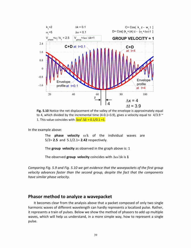
t = 3.9 Fig. 5.10 Notice the net displacement of the valley of the envelope is approximately equal to 4, which divided by the incremental time (4-0.1=3.9), gives a velocity equal to 4/3.9 ~
1. This value coincides with / k = 0.1/0.1 =1.
In the example above:
The phase velocity k of the individual waves are 5/2= 2.5 and 5.1/2.1= 2.42 respectively.
The group velocity as observed in the graph above is: 1
The observed group velocity coincides with k is 1
Comparing Fig. 5.9 and Fig. 5.10 we get evidence that the wavepackets of the first group velocity advances faster than the second group, despite the fact that the components have similar phase velocity.
Phasor method to analyze a wavepacket It becomes clear from the analysis above that a packet composed of only two single
harmonic waves of different wavelength can hardly represents a localized pulse. Rather, it represents a train of pulses. Below we show the method of phasors to add up multiple waves, which will help us understand, in a more simple way, how to represent a single pulse.

40
First, let’s try to understand qualitatively, from a phasors addition point of view, how a train of (multiple) pulses is formed.
Cos( ) Real axis
Im
phasor ei
Complex variable
plane
= kx-t
(kx-t)
Cos(kx-t) Real axis
Im
phasor e
i(kx-t)
Complex variable
plane
Fig. 5.10 A phasor representation in the complex plane.
Example: Let’s consider the wave (x,t) = Cos (kx – t) and analyze it at a
given fixed time (t= 0.1 for example)
Analysis using only real variable
First we plot the profile of the wave at t=0.1
-1
-0.5
0
0.5
1
0 5 10 15
C
D
E
x
(x,t) = Cos( k x - 0.1w ]
C
w=5
V=/ = 2.5
k=2
x
At t=0.1
Notice, as x changes the phase (kx – w 0.1) changes.
Analysis using complex variable, phasors

41
(kx – 0.1)
=Cos(kx – 0.1)
Real axis
Im
phasor
ei( k
x -
)
Complex
variable plane
Notice, as x changes the phase (kx – 0.1) changes.
CASE-1: Wavepacket composed of two waves
Let’s consider the addition of two harmonic waves
(x,t) = )()( t-xk Cos t- xk Cos BA
phase phase
(43) Real
where, without losing generality, we will assume BA kk . Also, let’s call
kkk AB .
To evaluate (43) we will work in the complex plane. Accordingly, to each wave we will associate a corresponding phasor,
~ (x,t) = )()( t-xk i t- xk i BA e e
Complex (44)
On the right side, ach phasor component has magnitude equal to 1. (But below we will draw them as it they had slightly different magnitude just for clarity)
The projection of the (complex) phasors along the horizontal axis will give the real-value
(x,t) we are looking for in (43). Notice in (44) that,
~ (x,t) = [xki xki BA e e ] e ti-
Hence, we can analyze first only the factor [xki xki BA e e ]. One can always add the
factor ti- e later on.
~ (x) = [xki xki BA e e ] (45)
42
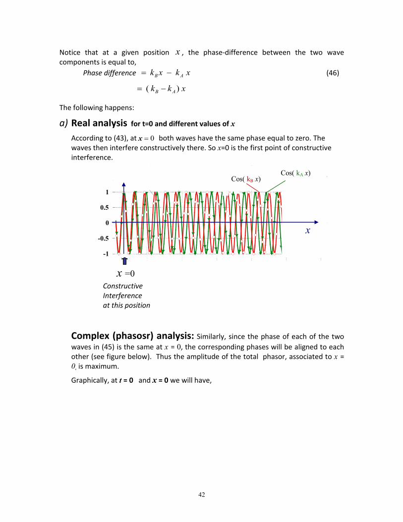
Notice that at a given position x , the phase-difference between the two wave components is equal to,
Phase difference x k xk AB (46)
xkk AB )(
The following happens:
a) Real analysis for t=0 and different values of x
According to (43), at 0x both waves have the same phase equal to zero. The waves then interfere constructively there. So x=0 is the first point of constructive interference.
-2
-1.5
-1
-0.5
0
0.5
1
1.5
2
0 10 20 30 40 50 60 70
At t=0.1C
D
E
z
D= Cos[ (+ z - (
t ]
C= Cos( k1 z - w
1 t ]
DC
Region of
constructive interference
=5 = 0.25
V=/ k
1 = 2.5
k1=2 k = 0.1
Region of
constructive interference
INDIVIDUAL WAVES
Cos( kB x) Cos( kA x)
x =0
x
Constructive Interference at this position
Complex (phasosr) analysis: Similarly, since the phase of each of the two
waves in (45) is the same at x = 0, the corresponding phases will be aligned to each other (see figure below). Thus the amplitude of the total phasor, associated to x = 0, is maximum.
Graphically, at t = 0 and x = 0 we will have,
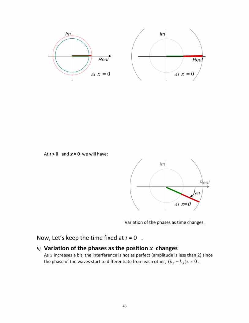
43
At x = 0 Real
Real
Im
At x = 0
Real
Im
At t > 0 and x = 0 we will have:
Real
t
At x=0
Real
Im
Variation of the phases as time changes.
Now, Let’s keep the time fixed at t = 0 .
b) Variation of the phases as the position x changes
As x increases a bit, the interference is not as perfect (amplitude is less than 2) since
the phase of the waves start to differentiate from each other; 0)( xkk AB .

44
kB x
kA x
At x=0 At x≠0
Real
Im
Real
Im
Fig. 5.11 Analysis of wave addition by phasors in the complex plane. For clarity, the magnitude of one of the phasors has been drawn larger than the other one. Notice, once a value of x is chosen and left fixed, as the time advances all the
phasors will rotate clockwise at angular velocity . kB x
kA x
kB x - kA x
c) As x increases, it will reach a particular value 1xx that makes the phase
difference between the waves equal to 2. The value of x1 is determined by the
condition, 2)( 1xkk AB .That is, the waves interfere constructively again at
kx /21 , where kkk AB .
kB x
kA x
Δk2π xx At 1 /
kkk AB
kA x1
kB x1
The phasors align again
Fig. 5.12 Left: In general, at arbitrary value of x, the phasors do not coincide. Right: At a particular specific value x=x1, both phasors coincide, thus giving a maximum value to the sum of the waves (at that location.) The phasors diagram also makes clear that as x keeps increasing, constructive interference will also occur at multiple values of x1.
45
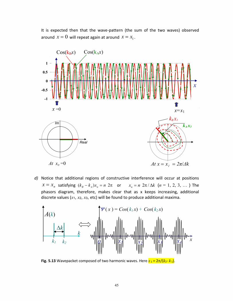
It is expected then that the wave-pattern (the sum of the two waves) observed
around 0x will repeat again at around 1xx .
-2
-1.5
-1
-0.5
0
0.5
1
1.5
2
0 10 20 30 40 50 60 70
At t=0.1C
D
E
z
D= Cos[ (+ z - (
t ]
C= Cos( k1 z - w
1 t ]
DC
Region of
constructive interference
=5 = 0.25
V=/ k
1 = 2.5
k1=2 k = 0.1
Region of
constructive interference
INDIVIDUAL WAVES
x
Cos(kBx) Cos(kAx)
x =0 x=x1
At xo =0
Real
Im
Δk2π xx At 1 /
kA x1
kB x1
d) Notice that additional regions of constructive interference will occur at positions
nxx satisfying 2)( nxkk nAB or knxn /2 (n = 1, 2, 3, … ) The
phasors diagram, therefore, makes clear that as x keeps increasing, additional discrete values (x1, x2, x3, etc) will be found to produce additional maxima.
x
k
A(k)
k
x2 x3 x1
( x )= Cos( k1 x) + Cos( k2 x)
k1 k2 0 x4
Fig. 5.13 Wavepacket composed of two harmonic waves. Here x 1 = 2/(k2- k 1).
46
Case II: A wavepacket composed of several harmonic waves
When adding several harmonic waves (x) =
M
iii xkCosA
1
)( , with M >2, the
condition for having repeated regions of constructive interference still can occurs. In effect,
First, there will be of course a constructive interference around x=0.
The next position x=x1 where maximum interference occurs will be one where the following condition is fulfilled
(ki - kj) x1 = (integer)ij 2 (47)
for all the ij combinations, with i and j = 1, 2, 3, … , M.
When condition (47) is fulfilled, all the corresponding phasors coincide, thus giving a maximum of amplitude for the wavepacket at x=x1.
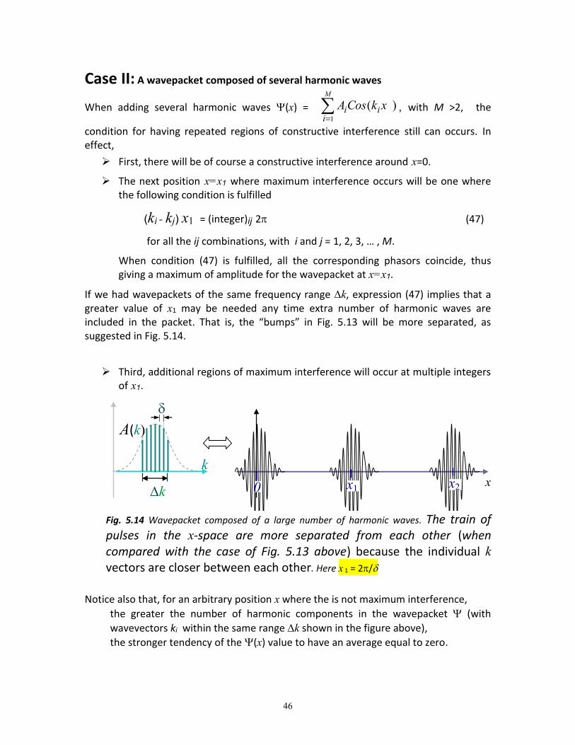
If we had wavepackets of the same frequency range k, expression (47) implies that a greater value of x1 may be needed any time extra number of harmonic waves are included in the packet. That is, the “bumps” in Fig. 5.13 will be more separated, as suggested in Fig. 5.14.
Third, additional regions of maximum interference will occur at multiple integers of x1.
x
k
A(k) ko
k x1 0 x2
Fig. 5.14 Wavepacket composed of a large number of harmonic waves. The train of pulses in the x-space are more separated from each other (when compared with the case of Fig. 5.13 above) because the individual k vectors are closer between each other. Here x 1 = 2/
Notice also that, for an arbitrary position x where the is not maximum interference,
the greater the number of harmonic components in the wavepacket (with
wavevectors ki within the same range k shown in the figure above),
the stronger tendency of the (x) value to have an average equal to zero.

47
Since the other maxima of interference occur at multiple values of x1, we expect,
therefore, that the greater number of k-values (within the
same range k), the more separated from each other will be the regions of constructive interference. This is shown in Fig.
5.14.
Case: Wavepacket composed of an infinite number of harmonic waves
Adding more and more wavevectors k (still all of them within the same range k show in the figure below)) will make the value of x1 to become greater and greater. As we consider a continuum variation of k, the value of x1 will become infinite. That is, we will obtain just one pulse.
x k
ko
k
A(k)
x
0
Fig. 5.15 Wavepacket composed of wavevectors k within a continuum range
k produces a single pulse.
What about the variation of the pulse-size as increases?
Fig. 5.15 above already suggests that the size should decrease. In effect, as the number of harmonic waves increases, the multiple addition of waves tends to average out to zero, unless x =0 or x had a very small value; that is the pulse becomes narrower.
Thus, we now can understand better the property stated in a previous paragraphs above (see expression (29) above, where the properties of the Fourier transform were being discussed.)
the more localized the function the broader its spectral response; and vice versa.
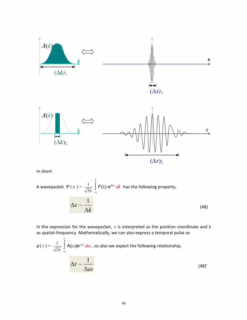
In effect, notice in the previous figure that if we were to increase the range k , the
corresponding range x of values of the x coordinate for which all the harmonic wave component can approximately interfere constructively would be reduced; and vice versa.
48
x k ko
k)1
A(k)
x)1
x k
k)2
A(k)
(x)2
In short:
A wavepacket ( x )= 2
1
F(k) eik x dk has the following property,
k
x
1
~ (48)
In the expression for the wavepacket, x is interpreted as the position coordinate and k
as spatial-frequency. Mathematically, we can also express a temporal pulse as
( t )= 2
1
A()eit d , so also we expect the following relationship,
1
~t (48)’

49
Expressions (48) and (48)’ are general properties of the Fourier analysis of waves. In principle, they have nothing to do with Quantum Mechanics.
We will see later that one way to describe QM is within the framework of Fourier
analysis. In this context, some of the mathematical terms ( and , to be more specific) are identified (via the de Broglie wave-particle duality hypothesis, to be expressed below) with the particle’s physical variables (p and E). Once this is done, then p and E) become subjected to the relationship indicated in (48) and (48)’.
The fact that physical variables are subjected to the relationships like in (48) and (48)’ constitute one of the cornerstones of Quantum Mechanics. We will explore this concept in the following section.
5.3 DESCRIBING the MOTION of a FREE PARTICLE in the context of the WAVE-PARTICLE DUALITY
According to Louis de Broglie, a particle of linear momentum p
and total energy E is associated with a wavelength an a frequency
given by,
ph / where is the wavelength of the wave associated with
the particle’s motion; and
E/hν the total energy E is related to the frequency ν of the wave associated with its motion.
where h is the Planck’s constant; h =6.6x10⁻³⁴ Js.
But the de Broglie postulate does not tell us how the wave-particle propagates. If, for example, the particle were to be subjected to
forces, its momentum could change in a very complicate way, and potentially not a single wavelength would be associated to the particle (maybe many harmonic waves would be needed to localize the particle.) The de Broglie postulate does not allow predicting such dynamic response (the Schrodinger equation, to be introduced in subsequent chapters, does that.)
As a first attempt to describe the propagation of a particle (through the space and time) lets consider first the simple case of a free particle (free particle motion implies
that its momentum p and energy E remain constant.) Our task is to figure out the wavefunction that describes the motion of a free particle.
50
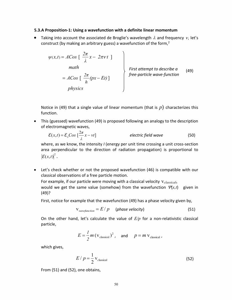
5.3.A Proposition-1: Using a wavefunction with a definite linear momentum
Taking into account the associated de Broglie’s wavelength and frequency , let’s construct (by making an arbitrary guess) a wavefunction of the form,2
physics
Et)(px ACos
math
t2 xλ
2π ACostx,ψ
h
2π
][
][)(
First attempt to describe a free-particle wave-function
(49)
Notice in (49) that a single value of linear momentum (that is p) characterizes this function.
This (guessed) wavefunction (49) is proposed following an analogy to the description of electromagnetic waves,
][),(2
νtxCostxλ
πo εε electric field wave (50)
where, as we know, the intensity I (energy per unit time crossing a unit cross-section area perpendicular to the direction of radiation propagation) is proportional to
2),( txε .
Let’s check whether or not the proposed wavefunction (46) is compatible with our
classical observations of a free particle motion.
For example, if our particle were moving with a classical velocity vclassical, would we get the same value (somehow) from the wavefunction (x,t) given in (49)?
First, notice for example that the wavefunction (49) has a phase velocity given by,
pEonwavefuncti /v (phase velocity) (51)
On the other hand, let’s calculate the value of E/p for a non-relativistic classical particle,
2
classical )v( mE2
1 , and classical vmp ,
which gives,
lassicalv2
1/ cpE (52)
From (51) and (52), one obtains,
51
classicalvv2
1onwavefuncti (53)
We realize here a disagreement between the velocity of the particle classicalv
and the phase velocity of the wave-particle onwavefunctiv that is supposed to represent
the particle.
This apparent shortcoming may be attributed to the fact that the proposed wave-function (49) has a definite momentum p (and thus an infinite spatial extension). A better selection of a wavefunction has to be made then in order to describe a particle more localized in space. That is explored in the next section.
5.3.B Proposition-2: Using a wave-packet as a wave-function
Let’s assume our classical particle of mass m is moving with velocity
oclassical vv classical velocity (54)
(or approximately equal to ov ).
Let’s build a wavefunction in terms of the value ov
To represent this particle, let’s build a Fourier wave-packet such that,
i) Its dominant harmonic component is one with
wavelength oo v/ mhλ , or
wavenumber ooo h)mk v/2(/2 (55)
or, equivalently, in terms of the variable p ,
ii) Its dominant harmonic component has
momentum oo vmpp (56)
That is, we would choose an amplitude A (p) that peaks when p is equal to the classical value of the particle’s momentum.
In the meantime, the width x and p of the wave packet are, otherwise, arbitrary.
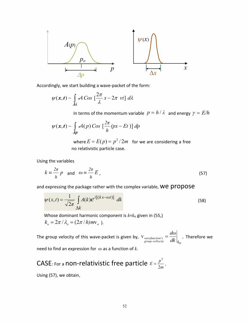
52
x x
p
po
A(p)
p
x)
Accordingly, we start building a wave-packet of the form:
dνtxCos
Δλ
tx ]22
[~),( A
In terms of the momentum variable λhp / and energy E/h
dp Et(pxCosph
2π Δp
tx ])[ )(~),( A
where mppEE 2/)( 2 for we are considering a free
no relativistic particle case.
Using the variables
pkh
2π and Eω
h
2π , (57)
and expressing the package rather with the complex variable, we propose
dkkAπ
tx
k
tωxkie
)][( )(
2
1),( (58)
Whose dominant harmonic component is k=ko given in (55,)
ooo h)mk v/2(/2 ).
The group velocity of this wave-packet is given by, okdk
dω
vellocity-groupson'wavefuncti v . Therefore we
need to find an expression for as a function of k.
CASE: For a non-relativistic free particle m
pE
2
2
.
Using (57), we obtain,

53
2m
kh
2m
pEkω
22
2πh
2π
h
2π)(
The group velocity of the wave-packet is given by,
m
kh
dk
dω o
ocitygroup-vellon'swavefuncti
ok 2v (59)
Using (57),
ovm
p
dk
dωv o
vellocity-groupsfunction'-wave
ok
(60)
Comparing this expression with expression (54), we realize that the wavepacket (58) represents better the non-relativistic particle, since the classical velocity is recovered through the group-velocity of the wavefunction.
The multiple-frequency wave-packet (58), instead of the single frequency expression (49,) represents better the particle since, at least for the moment, its group-velocity coincides with classical velocity of the particle.
Consequences: THE PARAGRAPH BELOW IS VERY IMPORTANT!
Notice, if a wave-packet (composed of harmonic waves with momentum-values p
within a given range p) is going to represent a particle, then, according to the Fourier
analysis there will be a corresponding extension x (wavepacket spatial width), which could be interpreted as the particle’s position. That is, there will not be a definite ‘exact’ position to be associated with the particle, but rather a range of possible values (within
x.) In short, there will be an uncertainty in the particle’s position.
In addition, if the Fourier analysis is providing the right tool to make connections between the wave-mechanics and the expected classical results (for example, allowing us to identify the classical velocity with the wave-packet’s group velocity) then we should be bounded by the other consequences inherent in the Fourier analysis. One of
them, for example, is that k
x
1
~ (see statement (29) and expression (48) and (48)’
above), which has profound consequences in our view of the mechanics governing Nature.
Indeed, from (53) ph
k
2
; thus k
x
1
~ implies pp
h
x
2
1~
, where
we have defined 2/h .
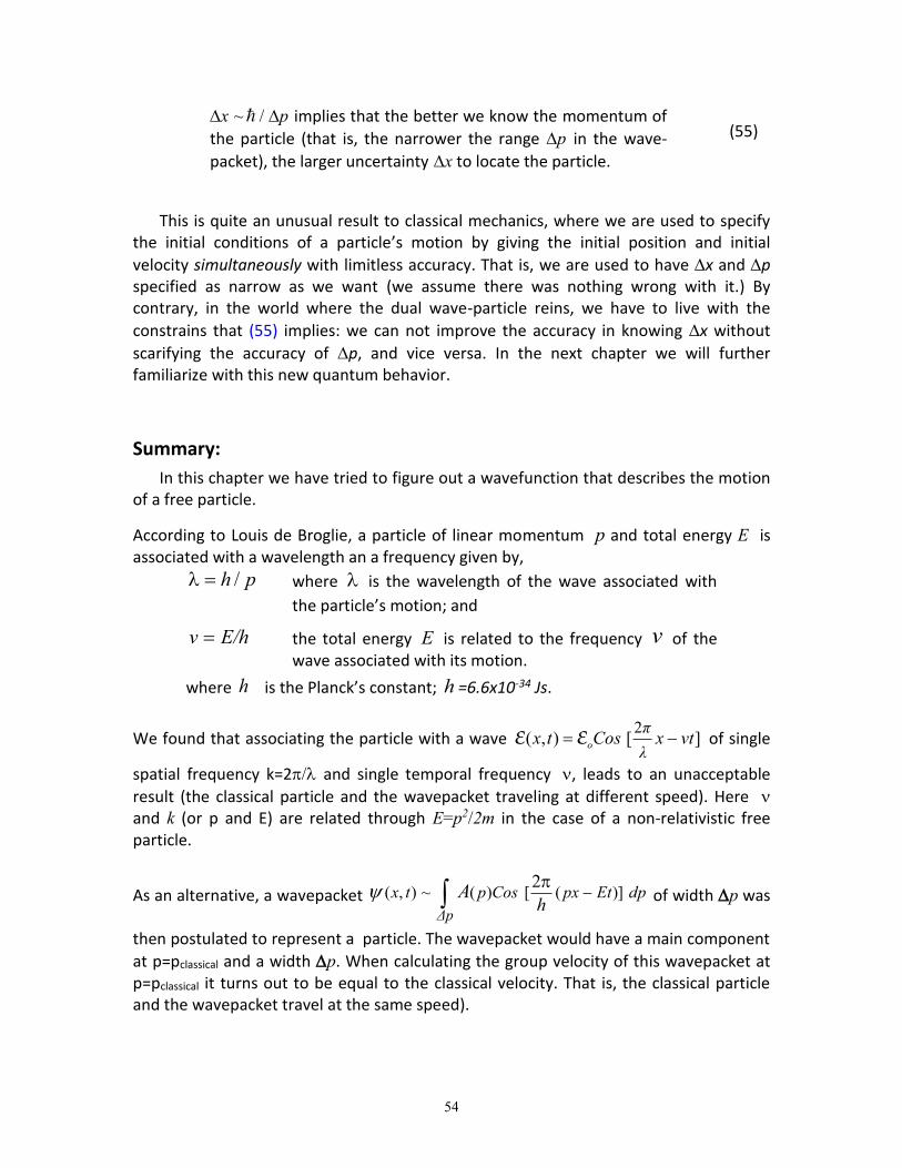
54
x ~ /p implies that the better we know the momentum of
the particle (that is, the narrower the range p in the wave-
packet), the larger uncertainty x to locate the particle.
(55)
This is quite an unusual result to classical mechanics, where we are used to specify the initial conditions of a particle’s motion by giving the initial position and initial
velocity simultaneously with limitless accuracy. That is, we are used to have x and p specified as narrow as we want (we assume there was nothing wrong with it.) By contrary, in the world where the dual wave-particle reins, we have to live with the
constrains that (55) implies: we can not improve the accuracy in knowing x without
scarifying the accuracy of p, and vice versa. In the next chapter we will further familiarize with this new quantum behavior.
Summary:
In this chapter we have tried to figure out a wavefunction that describes the motion of a free particle.
According to Louis de Broglie, a particle of linear momentum p and total energy E is associated with a wavelength an a frequency given by,
ph / where is the wavelength of the wave associated with
the particle’s motion; and
E/hν the total energy E is related to the frequency ν of the wave associated with its motion.
where h is the Planck’s constant; h =6.6x10⁻³⁴ Js.
We found that associating the particle with a wave ][),(2
νtxCostxλ
πo εε of single
spatial frequency k=2 and single temporal frequency , leads to an unacceptable
result (the classical particle and the wavepacket traveling at different speed). Here and k (or p and E) are related through E=p2/2m in the case of a non-relativistic free particle.
As an alternative, a wavepacket dpEtpxCosptx
Δph
A
)]([)(~),(2
of width p was
then postulated to represent a particle. The wavepacket would have a main component
at p=pclassical and a width p. When calculating the group velocity of this wavepacket at p=pclassical it turns out to be equal to the classical velocity. That is, the classical particle and the wavepacket travel at the same speed).

55
APPENDIX
Variations in the wavepacket for different spectral contents Credit graphic results: Joseph Scotto
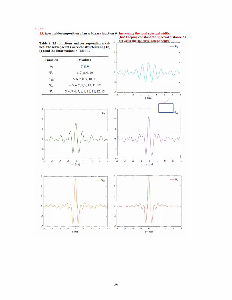
56
CASE
57
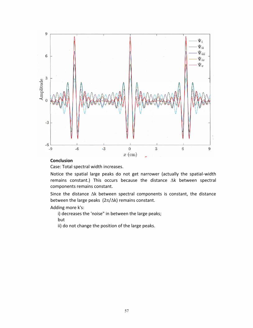
Conclusion Case: Total spectral width increases.
Notice the spatial large peaks do not get narrower (actually the spatial-width
remains constant.) This occurs because the distance k between spectral components remains constant.
Since the distance k between spectral components is constant, the distance
between the large peaks (2/k) remains constant.
Adding more k's: i) decreases the 'noise" in between the large peaks; but ii) do not change the position of the large peaks.
58
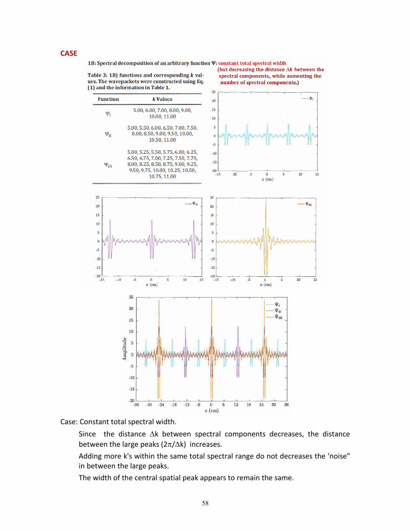
CASE
Case: Constant total spectral width.
Since the distance k between spectral components decreases, the distance
between the large peaks (2/k) increases.
Adding more k's within the same total spectral range do not decreases the 'noise" in between the large peaks.
The width of the central spatial peak appears to remain the same.
59
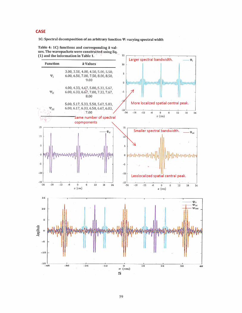
CASE
60
OVERALL CONCLUSION
The granularity Dk (distance between spectral components) determines the distance between large peaks.
The total spectral width determines the noise between peaks and the width of the spatial central peak.
1 A more general concept of the wave-particle duality is the PRINCIPE of
COMPLEMENTARY. See, for example, the following excellent reference: M. O. Scully, B. G. Englert, and H. Walther. “Quantum Optical Test of Complementary.” Nature 351, 111 (1991).
2 Here we follow closely Quantum Physics, Eisberg and Resnick, Section 3.2