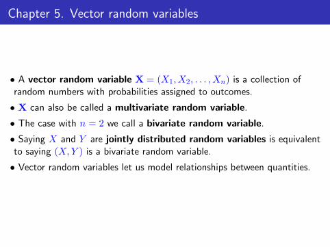
Chapter 5. Vector random variables

• A vector random variable X = (X1, X2, . . . , Xn) is a collection ofrandom numbers with probabilities assigned to outcomes.

• X can also be called a multivariate random variable.

• The case with n = 2 we call a bivariate random variable.

• Saying X and Y are jointly distributed random variables is equivalentto saying (X,Y ) is a bivariate random variable.

• Vector random variables let us model relationships between quantities.

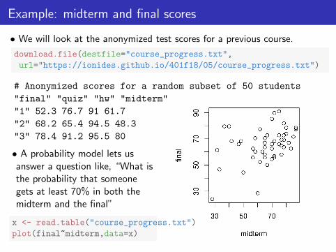
Example: midterm and final scores

• We will look at the anonymized test scores for a previous course.

download.file(destfile="course_progress.txt",

url="https://ionides.github.io/401f18/05/course_progress.txt")

# Anonymized scores for a random subset of 50 students

"final" "quiz" "hw" "midterm"

"1" 52.3 76.7 91 61.7

"2" 68.2 65.4 94.5 48.3

"3" 78.4 91.2 95.5 80

• A probability model lets usanswer a question like, “What isthe probability that someonegets at least 70% in both themidterm and the final”

x <- read.table("course_progress.txt")

plot(final~midterm,data=x)

The bivariate normal distribution and covariance

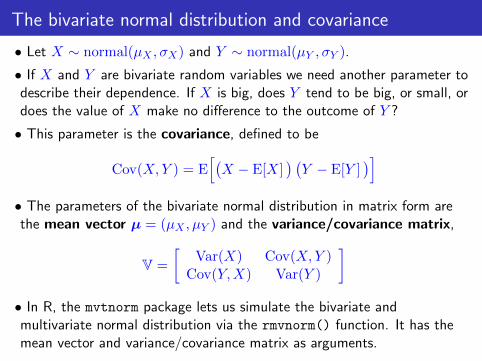
• Let X ∼ normal(µX , σX) and Y ∼ normal(µY , σY ).

• If X and Y are bivariate random variables we need another parameter todescribe their dependence. If X is big, does Y tend to be big, or small, ordoes the value of X make no difference to the outcome of Y ?

• This parameter is the covariance, defined to be

Cov(X,Y ) = E[(X − E[X]

) (Y − E[Y ]

)]• The parameters of the bivariate normal distribution in matrix form arethe mean vector µ = (µX , µY ) and the variance/covariance matrix,

V =

[Var(X) Cov(X,Y )

Cov(Y,X) Var(Y )

]• In R, the mvtnorm package lets us simulate the bivariate andmultivariate normal distribution via the rmvnorm() function. It has themean vector and variance/covariance matrix as arguments.

Experimenting with the bivariate normal distribution

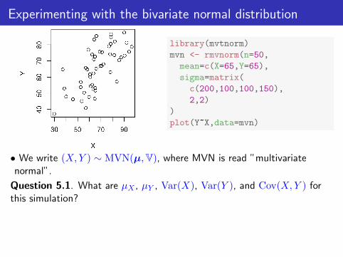
library(mvtnorm)

mvn <- rmvnorm(n=50,

mean=c(X=65,Y=65),

sigma=matrix(

c(200,100,100,150),

2,2)

)

plot(Y~X,data=mvn)

• We write (X,Y ) ∼ MVN(µ,V), where MVN is read ”multivariatenormal”.

Question 5.1. What are µX , µY , Var(X), Var(Y ), and Cov(X,Y ) forthis simulation?

The bivariate normal as a model for exam scores

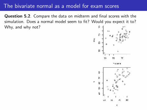
Question 5.2. Compare the data on midterm and final scores with thesimulation. Does a normal model seem to fit? Would you expect it to?Why, and why not?

More on covariance

• Covariance is symmetric: we see from the definition

Cov(X,Y ) = E[(X − E[X]

) (Y − E[Y ]

)]= E

[(Y − E[Y ]

) (X − E[X]

)]= Cov(Y,X)

• Also, we see from the definition that Cov(X,X) = Var(X).

• The sample covariance of n pairs of measurements(x1, y1), . . . , (xn, yn) is

cov(x,y) =1

n− 1

n∑i=1

(xi − x)(yi − y)

where x and y are the sample means of x = (x1, . . . , xn) andy = (y1, . . . , yn).

Scaling covariance to give correlation

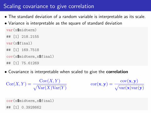
• The standard deviation of a random variable is interpretable as its scale.

• Variance is interpretable as the square of standard deviation

var(x$midterm)

## [1] 218.2155

var(x$final)

## [1] 169.7518

cov(x$midterm,x$final)

## [1] 75.61269

• Covariance is interpretable when scaled to give the correlation

Cor(X,Y ) =Cov(X,Y )√

Var(X)Var(Y )cor(x,y) =

cov(x,y)√var(x)var(y)

cor(x$midterm,x$final)

## [1] 0.3928662

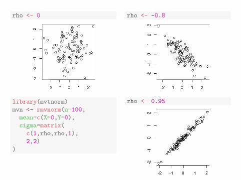
rho <- 0

library(mvtnorm)

mvn <- rmvnorm(n=100,

mean=c(X=0,Y=0),

sigma=matrix(

c(1,rho,rho,1),

2,2)

)

rho <- -0.8

rho <- 0.95

More on interpreting correlation

• Random variables with a correlation of ±1 (or data with a samplecorrelation of ±1) are called linearly dependent or colinear.

• Random variables with a correlation of 0 (or data with a samplecorrelation of 0) are uncorrelated.

• Random variables with a covariance of 0 are also uncorrelated!

Question 5.3. Suppose two data vectors x = (x1, . . . , xn) andy = (y1, . . . , yn) have been standardized. That is, each data point hashad the sample mean substracted and then been divided by the samplestandard deviation. You calculate cov(x,y) = 0.8. What is the samplecorrelation, cor(x,y)?

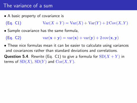
The variance of a sum

• A basic property of covariance is

(Eq. C1) Var(X + Y ) = Var(X) + Var(Y ) + 2 Cov(X,Y )

• Sample covariance has the same formula,

(Eq. C2) var(x + y) = var(x) + var(y) + 2 cov(x,y)

• These nice formulas mean it can be easier to calculate using variancesand covariances rather than standard deviations and correlations.

Question 5.4. Rewrite (Eq. C1) to give a formula for SD(X + Y ) interms of SD(X), SD(Y ) and Cor(X,Y ).

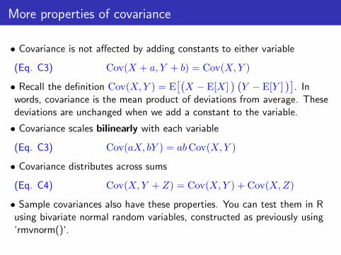
More properties of covariance

• Covariance is not affected by adding constants to either variable

(Eq. C3) Cov(X + a, Y + b) = Cov(X,Y )

• Recall the definition Cov(X,Y ) = E[(X − E[X]

) (Y − E[Y ]

)]. In

words, covariance is the mean product of deviations from average. Thesedeviations are unchanged when we add a constant to the variable.

• Covariance scales bilinearly with each variable

(Eq. C3) Cov(aX, bY ) = abCov(X,Y )

• Covariance distributes across sums

(Eq. C4) Cov(X,Y + Z) = Cov(X,Y ) + Cov(X,Z)

• Sample covariances also have these properties. You can test them in Rusing bivariate normal random variables, constructed as previously using‘rmvnorm()‘.

The variance/covariance matrix of vector random variables

• Let X = (X1, . . . , Xp) be a vector random variable. For any pair ofelements, say Xi and Xj , we can compute the usual scalar covariance,vij = Cov(Xi, Xj).

• The variance/covariance matrix V = [vij ]p×p collects together all thesecovariances.

V = Var(X) =

Cov(X1, X1) Cov(X1, X2) . . . Cov(X1, Xp)Cov(X2, X1) Cov(X2, X2) Cov(X2, Xp)

.... . .

...Cov(Xp, X1) Cov(Xp, X2) . . . Cov(Xp, Xp)

• The diagonal entries of V are vii = Cov(Xi, Xi) = Var(Xi) fori = 1, . . . , p so the variance/covariance matrix can be written as

V = Var(X) =

Var(X1) Cov(X1, X2) . . . Cov(X1, Xp)

Cov(X2, X1) Var(X2) Cov(X2, Xp)...

. . ....

Cov(Xp, X1) Cov(Xp, X2) . . . Var(Xp)

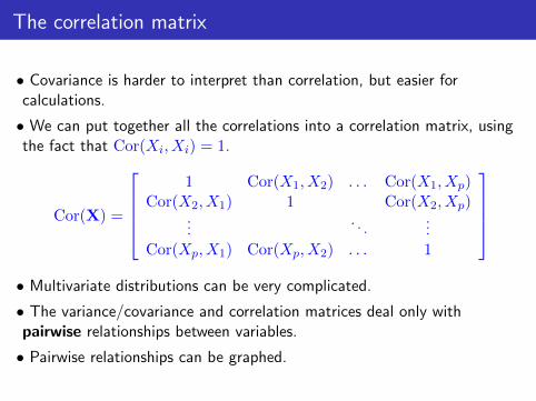
The correlation matrix

• Covariance is harder to interpret than correlation, but easier forcalculations.

• We can put together all the correlations into a correlation matrix, usingthe fact that Cor(Xi, Xi) = 1.

Cor(X) =

1 Cor(X1, X2) . . . Cor(X1, Xp)

Cor(X2, X1) 1 Cor(X2, Xp)...

. . ....

Cor(Xp, X1) Cor(Xp, X2) . . . 1

• Multivariate distributions can be very complicated.

• The variance/covariance and correlation matrices deal only withpairwise relationships between variables.

• Pairwise relationships can be graphed.

The sample variance/covariance matrix

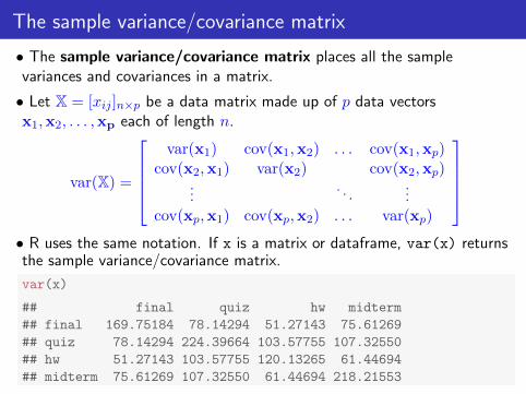
• The sample variance/covariance matrix places all the samplevariances and covariances in a matrix.

• Let X = [xij ]n×p be a data matrix made up of p data vectorsx1,x2, . . . ,xp each of length n.

var(X) =

var(x1) cov(x1,x2) . . . cov(x1,xp)

cov(x2,x1) var(x2) cov(x2,xp)...

. . ....

cov(xp,x1) cov(xp,x2) . . . var(xp)

• R uses the same notation. If x is a matrix or dataframe, var(x) returnsthe sample variance/covariance matrix.

var(x)

## final quiz hw midterm

## final 169.75184 78.14294 51.27143 75.61269

## quiz 78.14294 224.39664 103.57755 107.32550

## hw 51.27143 103.57755 120.13265 61.44694

## midterm 75.61269 107.32550 61.44694 218.21553

The sample correlation matrix

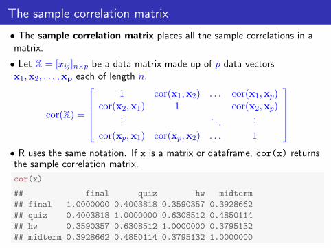
• The sample correlation matrix places all the sample correlations in amatrix.

• Let X = [xij ]n×p be a data matrix made up of p data vectorsx1,x2, . . . ,xp each of length n.

cor(X) =

1 cor(x1,x2) . . . cor(x1,xp)

cor(x2,x1) 1 cor(x2,xp)...

. . ....

cor(xp,x1) cor(xp,x2) . . . 1

• R uses the same notation. If x is a matrix or dataframe, cor(x) returnsthe sample correlation matrix.

cor(x)

## final quiz hw midterm

## final 1.0000000 0.4003818 0.3590357 0.3928662

## quiz 0.4003818 1.0000000 0.6308512 0.4850114

## hw 0.3590357 0.6308512 1.0000000 0.3795132

## midterm 0.3928662 0.4850114 0.3795132 1.0000000

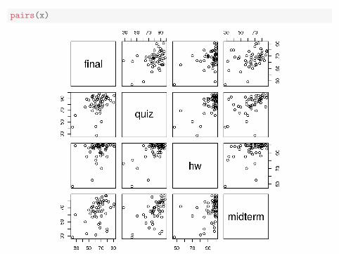
pairs(x)

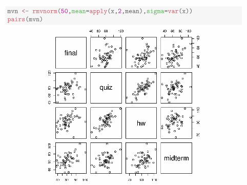
mvn <- rmvnorm(50,mean=apply(x,2,mean),sigma=var(x))

pairs(mvn)

Question 5.5. From looking at the scatterplots, what are the strengthsand weaknesses of a multivariate normal model for test scores in thiscourse?

Question 5.6. To what extent is it appropriate to summarize the data bythe mean and variance/covariance matrix (or correlation matrix) when thenormal approximation is dubious?

Linear combinations

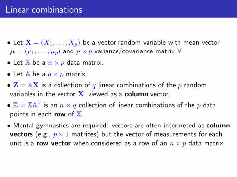
• Let X = (X1, . . . , Xp) be a vector random variable with mean vectorµ = (µ1, . . . , µp) and p× p variance/covariance matrix V.

• Let X be a n× p data matrix.

• Let A be a q × p matrix.

• Z = AX is a collection of q linear combinations of the p randomvariables in the vector X, viewed as a column vector.

• Z = XAt is an n× q collection of linear combinations of the p datapoints in each row of X.

• Mental gymnastics are required: vectors are often interpreted as columnvectors (e.g., p× 1 matrices) but the vector of measurements for eachunit is a row vector when considered as a row of an n× p data matrix.

Variables of length p as column vectors or row vectors

Question 5.7. How would you construct a simulated data matrix Zsim

from n realizations Z1, . . . ,Zn of the random column vector Z = AX?Hint: You are expected to write a matrix constructing Zsim by stackingtogether Z1, . . . ,Zn. Be careful with transposes and keep track ofdimensions. Recall that Zsim should be n× p.

Expectation and variance of linear combinations

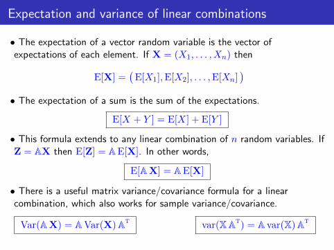
• The expectation of a vector random variable is the vector ofexpectations of each element. If X = (X1, . . . , Xn) then

E[X] =(

E[X1],E[X2], . . . ,E[Xn])

• The expectation of a sum is the sum of the expectations.

E[X + Y ] = E[X] + E[Y ]

• This formula extends to any linear combination of n random variables. IfZ = AX then E[Z] = AE[X]. In other words,

E[AX] = AE[X]

• There is a useful matrix variance/covariance formula for a linearcombination, which also works for sample variance/covariance.

Var(AX) = AVar(X)At var(XAt) = A var(X)At

Exercises with the matrix variance/covariance formula

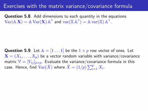
Question 5.8. Add dimensions to each quantity in the equationsVar(AX) = AVar(X)At and var(XAt) = A var(X)At.

Question 5.9. Let A = [1 . . . 1] be the 1 × p row vector of ones. LetX = (X1, . . . , Xp) be a vector random variable with variance/covariancematrix V = [Vij ]p×p. Evaluate the variance/covariance formula in thiscase. Hence, find Var(X) where X = (1/p)

∑pi=1Xi.

Testing the variance/covariance formula

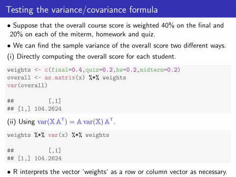
• Suppose that the overall course score is weighted 40% on the final and20% on each of the miterm, homework and quiz.

• We can find the sample variance of the overall score two different ways.

(i) Directly computing the overall score for each student.

weights <- c(final=0.4,quiz=0.2,hw=0.2,midterm=0.2)

overall <- as.matrix(x) %*% weights

var(overall)

## [,1]

## [1,] 104.2624

(ii) Using var(XAt) = A var(X)At.

weights %*% var(x) %*% weights

## [,1]

## [1,] 104.2624

• R interprets the vector ‘weights‘ as a row or column vector as necessary.

Independence

• Two events E and F are independent if

P(E and F ) = P(E) × P(F )

Worked example 5.1. Suppose we have a red die and a blue die. Theyare idea fair dice, so the values should be independent. What is the chancethey both show a six?(a) Using the definition of independence.

(b) By considering equally likely outcomes, without using the definition.

• The multiplication rule agrees with an intuitive idea of independence.

Independence of random variables

• X and Y are independent random variables if, for any intervals [a, b]and [c, d],

P(a < X < b and c < Y < d) = P(a < X < b) × P(c < Y < d)

• This definition extends to vector random variables. X = (X1, . . . , Xn) isa vector of independent random variables if for any collection ofintervals [ai, bi], 1 ≤ i ≤ n,

P(a1<X1 < b1, . . . , an<Xn<bn) = P(a1<X1<b1) × · · · × P(an<Xn<bn)

• X = (X1, . . . , Xn) is a vector of independent identically distributed(iid) random variables if, in addition, each element of X has the samedistribution.

• “X1, . . . , Xn are n random variables with the normal(µ, σ) distribution”is written more formally as

“Let X1, . . . , Xn ∼ iid normal(µ, σ).”

Independent vs uncorrelated

• If X and Y are independent they are uncorrelated.

• The converse is not necessarily true.

• For normal random variables, the converse is true.

• If X and Y are bivariate normal random variables, and Cov(X,Y ) = 0,then X and Y are independent.

• The following slide demonstrated the possibility of being uncorrelatedbut not independent (for non-normal random variables).

• If the scatter plot of two variables looks normal and their samplecorrelation is small, the variables are appropriately modeled asindependent.

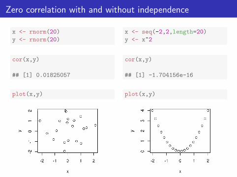
Zero correlation with and without independence

x <- rnorm(20)

y <- rnorm(20)

cor(x,y)

## [1] 0.01825057

plot(x,y)

x <- seq(-2,2,length=20)

y <- x^2

cor(x,y)

## [1] -1.704156e-16

plot(x,y)

The measurement error model

• Let ε = (ε1, ε2, . . . , εn) be a vector consisting of n independent normalrandom variables, each with mean zero and variance σ2.

• This is a common model for measurement error on n measurements.

• The mean vector and variance/covariance matrix are

E[ε] = 0, Var(ε) = σ2I

where 0 = (0, . . . , 0) and I is the n× n identity matrix.

• For the measurement error model, we break our usual rule of using uppercase letters for random variables.

• We can write ε ∼ MVN(0, σ2I) or ε ∼ iid normal(0, σ).

• ε models unbiased measurements (meaning E[εi] = 0) subject toadditive Gaussian error.

Example: 5 repeated measurements x1, . . . , x5 of the speed of light couldbe modeled as Xi = µ+ εi for i = 1, . . . , 5, where µ is the unknown truevalue of this quantity.

A probability model for the linear model

• First recall the sample version of the linear model, which is

y = Xb + e,

where y is the measured response, X is an n× p matrix of explanatoryvariables, b is chosen by least squares, and e is the vector of residuals.

• We want to build a random vector Y that provides a probability modelfor the data y. We write this as

Y = Xβ + ε

where X is the explanatory matrix, β = (β1, . . . , βp) is an unknowncoefficient vector (we don’t know the true population coefficient!) and εis Gaussian measurement error with E[ε] = 0 and Var(ε) = σ2I.• Our probability model asserts that the process which generated theresponse data y was like drawing a random vector Y constructed using arandom measurement error model with known matrix X for some fixedbut unknown value of β.

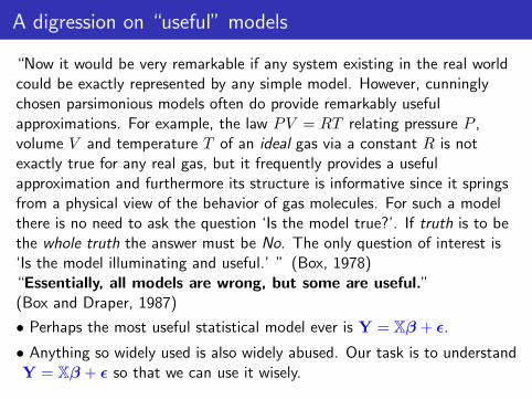
A digression on “useful” models

“Now it would be very remarkable if any system existing in the real worldcould be exactly represented by any simple model. However, cunninglychosen parsimonious models often do provide remarkably usefulapproximations. For example, the law PV = RT relating pressure P ,volume V and temperature T of an ideal gas via a constant R is notexactly true for any real gas, but it frequently provides a usefulapproximation and furthermore its structure is informative since it springsfrom a physical view of the behavior of gas molecules. For such a modelthere is no need to ask the question ‘Is the model true?’. If truth is to bethe whole truth the answer must be No. The only question of interest is‘Is the model illuminating and useful.’ ” (Box, 1978)“Essentially, all models are wrong, but some are useful.”(Box and Draper, 1987)

• Perhaps the most useful statistical model ever is Y = Xβ + ε.

• Anything so widely used is also widely abused. Our task is to understandY = Xβ + ε so that we can use it wisely.

Expectation and variance/covariance of Y

• Recall the linear model Y = Xβ + ε where ε ∼ MVN(0, σ2I).

Question 5.10. What is the expected value, E[Y]?

Question 5.11. What is the variance/covariance matrix, Var(Y)?

Expectation of the least squares coefficient

Worked example 5.2. Let β =(XtX

)−1XtY. This is the probability

model for the sample least squares coefficient b =(XtX

)−1Xty. Use

linearity to calculate E[β].

Solution:E[β] = E

[ (XtX

)−1XtY]

=(XtX

)−1Xt E[Y]

=(XtX

)−1XtXβ

= β

• Interpretation: If the data y are well modeled as a draw from theprobability model Y = Xβ + ε, then the least squares estimate b is wellmodeled by a random vector with mean β.

Variance/covariance matrix of the least squares coefficients

Question 5.12. Consider the linear model Y = Xβ + ε with E[ε] = 0 andVar(ε) = σ2I. Use the formula Var(AY) = AVar(Y)At to find Var(β).Hint: what should be our choice of A so that β = AY?

Standard errors for coefficients in the linear model

• The formula Var(β) = σ2(XtX

)−1needs extra work to be useful for

data analysis.

• In practice, we know the model matrix X but we don’t know themeasurement standard deviation σ.

• An estimate of the measurement standard deviation is the samplestandard deviation of the residuals.

• For y = Xb + e with X being n× p, an estimate of σ is

s =√

1n−p

∑ni=1

(yi − yi

)2=√

1n−p

∑ni=1

(yi − [Xb]i

)2• We will discuss later why we choose to divide by n− p.

• The standard error of bk for k = 1, . . . , p is

SE(bk) = s√[(

XtX)−1]

kkwhich is an estimate of

√[Var(β)

]kk

.

• These standard errors are calculated by lm() in R.

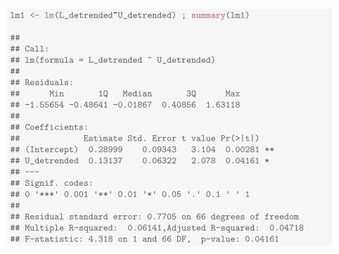
lm1 <- lm(L_detrended~U_detrended) ; summary(lm1)

##

## Call:

## lm(formula = L_detrended ~ U_detrended)

##

## Residuals:

## Min 1Q Median 3Q Max

## -1.55654 -0.48641 -0.01867 0.40856 1.63118

##

## Coefficients:

## Estimate Std. Error t value Pr(>|t|)

## (Intercept) 0.28999 0.09343 3.104 0.00281 **

## U_detrended 0.13137 0.06322 2.078 0.04161 *

## ---

## Signif. codes:

## 0 '***' 0.001 '**' 0.01 '*' 0.05 '.' 0.1 ' ' 1

##

## Residual standard error: 0.7705 on 66 degrees of freedom

## Multiple R-squared: 0.06141,Adjusted R-squared: 0.04718

## F-statistic: 4.318 on 1 and 66 DF, p-value: 0.04161

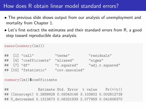
How does R obtain linear model standard errors?

• The previous slide shows output from our analysis of unemployment andmortality from Chapter 1.

• Let’s first extract the estimates and their standard errors from R, a goodstep toward reproducible data analysis.

names(summary(lm1))

## [1] "call" "terms" "residuals"

## [4] "coefficients" "aliased" "sigma"

## [7] "df" "r.squared" "adj.r.squared"

## [10] "fstatistic" "cov.unscaled"

summary(lm1)$coefficients

## Estimate Std. Error t value Pr(>|t|)

## (Intercept) 0.2899928 0.09343146 3.103802 0.002812739

## U_detrended 0.1313673 0.06321939 2.077959 0.041606370

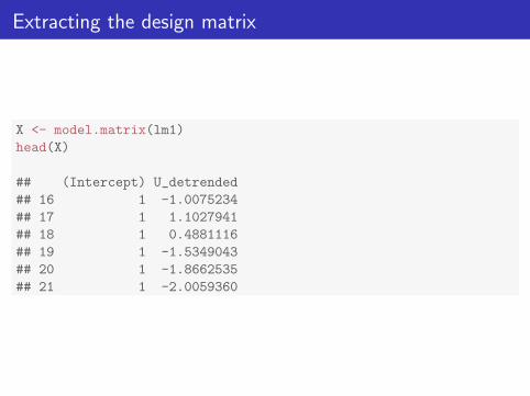
Extracting the design matrix

X <- model.matrix(lm1)

head(X)

## (Intercept) U_detrended

## 16 1 -1.0075234

## 17 1 1.1027941

## 18 1 0.4881116

## 19 1 -1.5349043

## 20 1 -1.8662535

## 21 1 -2.0059360

Computing the standard errors directly

s <- sqrt(sum(resid(lm1)^2)/(nrow(X)-ncol(X))) ; s

## [1] 0.7704556

V <- s^2 * solve(t(X)%*%X)

sqrt(diag(V))

## (Intercept) U_detrended

## 0.09343146 0.06321939

• This matches the standard errors generated by lm().

summary(lm1)$coefficients

## Estimate Std. Error t value Pr(>|t|)

## (Intercept) 0.2899928 0.09343146 3.103802 0.002812739

## U_detrended 0.1313673 0.06321939 2.077959 0.041606370

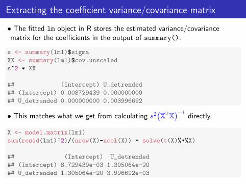
Extracting the coefficient variance/covariance matrix

• The fitted lm object in R stores the estimated variance/covariancematrix for the coefficients in the output of summary().

s <- summary(lm1)$sigma

XX <- summary(lm1)$cov.unscaled

s^2 * XX

## (Intercept) U_detrended

## (Intercept) 0.008729439 0.000000000

## U_detrended 0.000000000 0.003996692

• This matches what we get from calculating s2(XtX

)−1directly.

X <- model.matrix(lm1)

sum(resid(lm1)^2)/(nrow(X)-ncol(X)) * solve(t(X)%*%X)

## (Intercept) U_detrended

## (Intercept) 8.729439e-03 1.305064e-20

## U_detrended 1.305064e-20 3.996692e-03