Chapter 5 The Normal Curve. Histogram of Unemployment rates, States database.
22
Chapter 5 The Normal Curve
-
Upload
christiana-montgomery -
Category
Documents
-
view
225 -
download
2
Transcript of Chapter 5 The Normal Curve. Histogram of Unemployment rates, States database.

Chapter 5
The Normal Curve

Histogram of Unemployment rates, States database
Unemployment rate
6.506.005.505.004.504.003.503.002.502.00
14
12
10
8
6
4
2
0
Std. Dev = .95
Mean = 3.90
N = 50.00

Histogram of Abortion Rates, States Database
Abortions per 1000 women
45.0
42.5
40.0
37.5
35.0
32.5
30.0
27.5
25.0
22.5
20.0
17.5
15.0
12.5
10.0
7.5
5.0
2.5
10
8
6
4
2
0
Std. Dev = 9.12
Mean = 17.8
N = 50.00

Histogram of population growth rates from Nations database
CURRENT ANNUAL POPULATION GROWTH RATE
8.00
7.50
7.00
6.50
6.00
5.50
5.00
4.50
4.00
3.50
3.00
2.50
2.00
1.50
1.00
.50
0.00
-.50
-1.00
30
20
10
0
Std. Dev = 1.49
Mean = 1.73
N = 174.00

Histogram of suicide rates from Nations Study
SUICIDES PER 100,000 POP
42.5
40.0
37.5
35.0
32.5
30.0
27.5
25.0
22.5
20.0
17.5
15.0
12.5
10.0
7.5
5.0
2.5
0.0
14
12
10
8
6
4
2
0
Std. Dev = 8.62
Mean = 9.9
N = 69.00

Theoretical Normal Curve
Bell Shaped Unimodal Symmetrical Unskewed Mode,
Median, and Mean are same value
Normal Curve
68.26%
95.44%
99.72%

Theoretical Normal Curve
Distances on horizontal axis always cut off the same area. We can use this property to describe areas above or below any point

Theoretical Normal Curve General relationships:
±1 s = about 68% ±2 s = about 95% ±3 s = about 99%

Theoretical Normal Curve
-5 -4 -3 -2 -1 0 1 2 3 4 5
68.26%
95.44%
99.72%

Unemployment rates againMean=3.9%, s=.95
3.9+/-.95 gives a range of 2.95-4.85, which includes 34 states
3.9+/-1.9 gives a range of 2.0-5.8, which includes 29 states
Unemployment rate
6.506.005.505.004.504.003.503.002.502.00
14
12
10
8
6
4
2
0
Std. Dev = .95
Mean = 3.90
N = 50.00

Using the Normal Curve: Z Scores To find areas, first compute Z scores. The formula changes a “raw” score (Xi) to
a standardized score (Z).

Using Appendix A to Find Areas Below a Score
Appendix A can be used to find the areas above and below a score.
First compute the Z score, taking careful note of the sign of the score.
Draw a picture of the normal curve and shade in the area in which you are interested.

Using Appendix A
b b
Appendix A has three columns. (a) = Z scores. (b) = areas between the score and the mean

Using Appendix A
Appendix A has three columns. ( c) = areas beyond the Z score
c c

Using Appendix A Find your Z score
in Column A. To find area below
a positive score: Add column b area
to .50. To find area above
a positive score Look in column c.
(a) (b) (c)
. . .
1.66 0.4515 0.0485
1.67 0.4525 0.0475
1.68 0.4535 0.0465
. . .
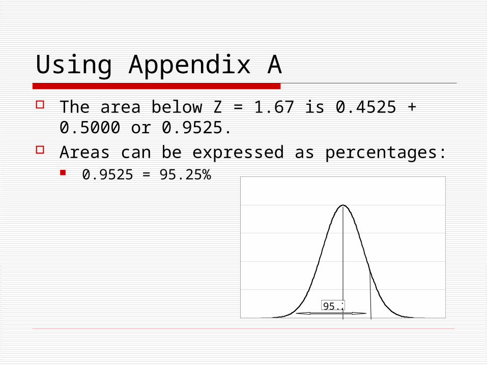
Using Appendix A The area below Z = 1.67 is 0.4525 +
0.5000 or 0.9525. Areas can be expressed as percentages:
0.9525 = 95.25%
95.2

Normal curve w z=1.67
95.25%

Using Appendix A What if the Z score
is negative (–1.67)? To find area below
a negative score: Look in column c.
To find area above a negative score Add column b .50
(a) (b) (c)
. . .
1.66 0.4515 0.0485
1.67 0.4525 0.0475
1.68 0.4535 0.0465
. . .

Using Appendix A The area below Z = - 1.67 is 0.475. Areas can be expressed as %: 4.75%.
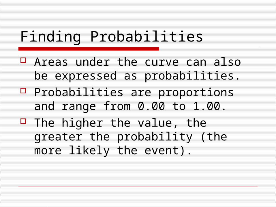
Finding Probabilities
Areas under the curve can also be expressed as probabilities.
Probabilities are proportions and range from 0.00 to 1.00.
The higher the value, the greater the probability (the more likely the event).

Finding Probabilities
If A distribution has: = 13 s = 4
What is the probability of randomly selecting a score of 19 or more?
X

Finding Probabilities
1. Find the Z score.2. For Xi = 19, Z =
1.50.3. Find area above in
column c.4. Probability is
0.0668 or 0.07.
(a) (b) (c)
. . .
1.49 0.4319 0.0681
1.50 0.4332 0.0668
1.51 0.4345 0.0655
. . .