Chapter 5 THE APPLICATION OF THE Z TRANSFORM 5.5.5 ...dsp/sup-materials/Slides/dsp-ch05-S5.5P.pdft...
Chapter 5 THE APPLICATION OF THE Z TRANSFORM 5.5.5 Frequency Response of Digital Filters Copyright c 2005 Andreas Antoniou Victoria, BC, Canada Email: [email protected] July 14, 2018 Frame # 1 Slide # 1 A. Antoniou Digital Signal Processing – Sec. 5.5.5
Transcript of Chapter 5 THE APPLICATION OF THE Z TRANSFORM 5.5.5 ...dsp/sup-materials/Slides/dsp-ch05-S5.5P.pdft...

Chapter 5THE APPLICATION OF THE Z TRANSFORM
5.5.5 Frequency Response of Digital Filters
Copyright c© 2005 Andreas AntoniouVictoria, BC, Canada
Email: [email protected]
July 14, 2018
Frame # 1 Slide # 1 A. Antoniou Digital Signal Processing – Sec. 5.5.5

Introduction
t In Sec. 5.5, it is shown that the steady-state response of a stableNth-order discrete-time system to a sinusoidal signal
x(nT ) = u(nT ) sinωnT
is another sinusoidal signal of the form
limnT→∞
y(nT ) = y(nT ) = M(ω) sin[ωnT + θ(ω)]
t The quantities
M(ω) = |H(e jωT )| and θ(ω) = argH(e jωT )
define the amplitude response and phase response, respectively, and
H(z)∣∣z=e jωT = H(e jωT ) = M(ω)e jθ(ω)
defines the frequency response.
Frame # 2 Slide # 2 A. Antoniou Digital Signal Processing – Sec. 5.5.5

Introduction
t In Sec. 5.5, it is shown that the steady-state response of a stableNth-order discrete-time system to a sinusoidal signal
x(nT ) = u(nT ) sinωnT
is another sinusoidal signal of the form
limnT→∞
y(nT ) = y(nT ) = M(ω) sin[ωnT + θ(ω)]
t The quantities
M(ω) = |H(e jωT )| and θ(ω) = argH(e jωT )
define the amplitude response and phase response, respectively, and
H(z)∣∣z=e jωT = H(e jωT ) = M(ω)e jθ(ω)
defines the frequency response.
Frame # 2 Slide # 3 A. Antoniou Digital Signal Processing – Sec. 5.5.5

Introduction Cont’d
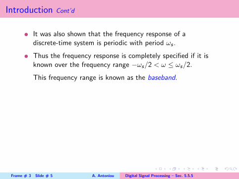
t It was also shown that the frequency response of adiscrete-time system is periodic with period ωs .
t Thus the frequency response is completely specified if it isknown over the frequency range −ωs/2 < ω ≤ ωs/2.
This frequency range is known as the baseband.t It can be easily shown that the amplitude response is an evenfunction and the phase response is an odd function of ω, i.e.,
M(−ω) = M(ω) and θ(−ω) = −θ(ω)
t Therefore, the frequency response is completely specified if itis known over the positive half of the baseband, i.e.,0 ≤ ω ≤ ωs/2.
Frame # 3 Slide # 4 A. Antoniou Digital Signal Processing – Sec. 5.5.5
Introduction Cont’d
t It was also shown that the frequency response of adiscrete-time system is periodic with period ωs .t Thus the frequency response is completely specified if it isknown over the frequency range −ωs/2 < ω ≤ ωs/2.
This frequency range is known as the baseband.
t It can be easily shown that the amplitude response is an evenfunction and the phase response is an odd function of ω, i.e.,
M(−ω) = M(ω) and θ(−ω) = −θ(ω)
t Therefore, the frequency response is completely specified if itis known over the positive half of the baseband, i.e.,0 ≤ ω ≤ ωs/2.
Frame # 3 Slide # 5 A. Antoniou Digital Signal Processing – Sec. 5.5.5

Introduction Cont’d
t It was also shown that the frequency response of adiscrete-time system is periodic with period ωs .t Thus the frequency response is completely specified if it isknown over the frequency range −ωs/2 < ω ≤ ωs/2.
This frequency range is known as the baseband.t It can be easily shown that the amplitude response is an evenfunction and the phase response is an odd function of ω, i.e.,
M(−ω) = M(ω) and θ(−ω) = −θ(ω)
t Therefore, the frequency response is completely specified if itis known over the positive half of the baseband, i.e.,0 ≤ ω ≤ ωs/2.
Frame # 3 Slide # 6 A. Antoniou Digital Signal Processing – Sec. 5.5.5

Introduction Cont’d
t It was also shown that the frequency response of adiscrete-time system is periodic with period ωs .t Thus the frequency response is completely specified if it isknown over the frequency range −ωs/2 < ω ≤ ωs/2.
This frequency range is known as the baseband.t It can be easily shown that the amplitude response is an evenfunction and the phase response is an odd function of ω, i.e.,
M(−ω) = M(ω) and θ(−ω) = −θ(ω)
t Therefore, the frequency response is completely specified if itis known over the positive half of the baseband, i.e.,0 ≤ ω ≤ ωs/2.
Frame # 3 Slide # 7 A. Antoniou Digital Signal Processing – Sec. 5.5.5

Introduction Cont’d
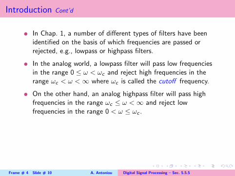
t In Chap. 1, a number of different types of filters have beenidentified on the basis of which frequencies are passed orrejected, e.g., lowpass or highpass filters.
t In the analog world, a lowpass filter will pass low frequenciesin the range 0 ≤ ω < ωc and reject high frequencies in therange ωc < ω <∞ where ωc is called the cutoff frequency.t On the other hand, an analog highpass filter will pass highfrequencies in the range ωc ≤ ω <∞ and reject lowfrequencies in the range 0 < ω ≤ ωc .
Frame # 4 Slide # 8 A. Antoniou Digital Signal Processing – Sec. 5.5.5

Introduction Cont’d
t In Chap. 1, a number of different types of filters have beenidentified on the basis of which frequencies are passed orrejected, e.g., lowpass or highpass filters.t In the analog world, a lowpass filter will pass low frequenciesin the range 0 ≤ ω < ωc and reject high frequencies in therange ωc < ω <∞ where ωc is called the cutoff frequency.
t On the other hand, an analog highpass filter will pass highfrequencies in the range ωc ≤ ω <∞ and reject lowfrequencies in the range 0 < ω ≤ ωc .
Frame # 4 Slide # 9 A. Antoniou Digital Signal Processing – Sec. 5.5.5
Introduction Cont’d
t In Chap. 1, a number of different types of filters have beenidentified on the basis of which frequencies are passed orrejected, e.g., lowpass or highpass filters.t In the analog world, a lowpass filter will pass low frequenciesin the range 0 ≤ ω < ωc and reject high frequencies in therange ωc < ω <∞ where ωc is called the cutoff frequency.t On the other hand, an analog highpass filter will pass highfrequencies in the range ωc ≤ ω <∞ and reject lowfrequencies in the range 0 < ω ≤ ωc .
Frame # 4 Slide # 10 A. Antoniou Digital Signal Processing – Sec. 5.5.5

Introduction Cont’d
t In the digital world, the filter is classified on the basis of itsamplitude response with respect to the positive half of thebaseband.
t Thus a digital lowpass filter will pass low frequencies in therange 0 ≤ ω < ωc and reject high frequencies in the rangeωc < ω < ωs/2 where ωc is the cutoff frequency, as in thecase of analog filters.t A digital highpass filter will pass high frequencies in the rangeωc ≤ ω < ωs/2 and reject low frequencies in the range0 < ω ≤ ωc .
Frame # 5 Slide # 11 A. Antoniou Digital Signal Processing – Sec. 5.5.5

Introduction Cont’d
t In the digital world, the filter is classified on the basis of itsamplitude response with respect to the positive half of thebaseband.t Thus a digital lowpass filter will pass low frequencies in therange 0 ≤ ω < ωc and reject high frequencies in the rangeωc < ω < ωs/2 where ωc is the cutoff frequency, as in thecase of analog filters.
t A digital highpass filter will pass high frequencies in the rangeωc ≤ ω < ωs/2 and reject low frequencies in the range0 < ω ≤ ωc .
Frame # 5 Slide # 12 A. Antoniou Digital Signal Processing – Sec. 5.5.5

Introduction Cont’d
t In the digital world, the filter is classified on the basis of itsamplitude response with respect to the positive half of thebaseband.t Thus a digital lowpass filter will pass low frequencies in therange 0 ≤ ω < ωc and reject high frequencies in the rangeωc < ω < ωs/2 where ωc is the cutoff frequency, as in thecase of analog filters.t A digital highpass filter will pass high frequencies in the rangeωc ≤ ω < ωs/2 and reject low frequencies in the range0 < ω ≤ ωc .
Frame # 5 Slide # 13 A. Antoniou Digital Signal Processing – Sec. 5.5.5
Introduction Cont’d
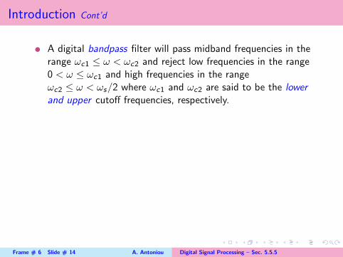
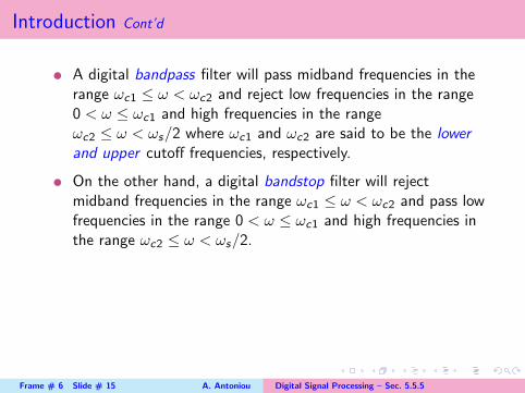
t A digital bandpass filter will pass midband frequencies in therange ωc1 ≤ ω < ωc2 and reject low frequencies in the range0 < ω ≤ ωc1 and high frequencies in the rangeωc2 ≤ ω < ωs/2 where ωc1 and ωc2 are said to be the lowerand upper cutoff frequencies, respectively.
t On the other hand, a digital bandstop filter will rejectmidband frequencies in the range ωc1 ≤ ω < ωc2 and pass lowfrequencies in the range 0 < ω ≤ ωc1 and high frequencies inthe range ωc2 ≤ ω < ωs/2.t In other words, the upper edge of the baseband in digitalsystems is analogous to infinite frequency in analog systems.
Frame # 6 Slide # 14 A. Antoniou Digital Signal Processing – Sec. 5.5.5
Introduction Cont’d
t A digital bandpass filter will pass midband frequencies in therange ωc1 ≤ ω < ωc2 and reject low frequencies in the range0 < ω ≤ ωc1 and high frequencies in the rangeωc2 ≤ ω < ωs/2 where ωc1 and ωc2 are said to be the lowerand upper cutoff frequencies, respectively.t On the other hand, a digital bandstop filter will rejectmidband frequencies in the range ωc1 ≤ ω < ωc2 and pass lowfrequencies in the range 0 < ω ≤ ωc1 and high frequencies inthe range ωc2 ≤ ω < ωs/2.
t In other words, the upper edge of the baseband in digitalsystems is analogous to infinite frequency in analog systems.
Frame # 6 Slide # 15 A. Antoniou Digital Signal Processing – Sec. 5.5.5

Introduction Cont’d
t A digital bandpass filter will pass midband frequencies in therange ωc1 ≤ ω < ωc2 and reject low frequencies in the range0 < ω ≤ ωc1 and high frequencies in the rangeωc2 ≤ ω < ωs/2 where ωc1 and ωc2 are said to be the lowerand upper cutoff frequencies, respectively.t On the other hand, a digital bandstop filter will rejectmidband frequencies in the range ωc1 ≤ ω < ωc2 and pass lowfrequencies in the range 0 < ω ≤ ωc1 and high frequencies inthe range ωc2 ≤ ω < ωs/2.t In other words, the upper edge of the baseband in digitalsystems is analogous to infinite frequency in analog systems.
Frame # 6 Slide # 16 A. Antoniou Digital Signal Processing – Sec. 5.5.5

Introduction Cont’d
t An arbitrary transfer function H(z) can be expressed in terms of itsmagnitude and angle as
H(z) = |H(z)|e j argH(z)
t If z is a complex variable of the form z = Re z + j Im z , then
|H(z)| = |Re H(z) + j Im H(z)|
and
argH(z) = tan−1Im H(z)
Re H(z)t These quantities represent surfaces over the z plane, which can berepresented by 3-dimensional plots.
Note: The magnitude function |H(z)| is, of course, a nonnegativequantity but argH(z) can be positive or negative.
Frame # 7 Slide # 17 A. Antoniou Digital Signal Processing – Sec. 5.5.5

Introduction Cont’d
t An arbitrary transfer function H(z) can be expressed in terms of itsmagnitude and angle as
H(z) = |H(z)|e j argH(z)
t If z is a complex variable of the form z = Re z + j Im z , then
|H(z)| = |Re H(z) + j Im H(z)|
and
argH(z) = tan−1Im H(z)
Re H(z)
t These quantities represent surfaces over the z plane, which can berepresented by 3-dimensional plots.
Note: The magnitude function |H(z)| is, of course, a nonnegativequantity but argH(z) can be positive or negative.
Frame # 7 Slide # 18 A. Antoniou Digital Signal Processing – Sec. 5.5.5

Introduction Cont’d
t An arbitrary transfer function H(z) can be expressed in terms of itsmagnitude and angle as
H(z) = |H(z)|e j argH(z)
t If z is a complex variable of the form z = Re z + j Im z , then
|H(z)| = |Re H(z) + j Im H(z)|
and
argH(z) = tan−1Im H(z)
Re H(z)t These quantities represent surfaces over the z plane, which can berepresented by 3-dimensional plots.
Note: The magnitude function |H(z)| is, of course, a nonnegativequantity but argH(z) can be positive or negative.
Frame # 7 Slide # 19 A. Antoniou Digital Signal Processing – Sec. 5.5.5

Introduction Cont’d
t An arbitrary transfer function H(z) can be expressed in terms of itsmagnitude and angle as
H(z) = |H(z)|e j argH(z)
t If z is a complex variable of the form z = Re z + j Im z , then
|H(z)| = |Re H(z) + j Im H(z)|
and
argH(z) = tan−1Im H(z)
Re H(z)t These quantities represent surfaces over the z plane, which can berepresented by 3-dimensional plots.
Note: The magnitude function |H(z)| is, of course, a nonnegativequantity but argH(z) can be positive or negative.
Frame # 7 Slide # 20 A. Antoniou Digital Signal Processing – Sec. 5.5.5

Introduction Cont’d
t If we let z = e jωT , i.e., if z assumes values on the unit circle|z | = 1, then 3-D plots of the form
– |H(e jωT )| versus e jωT and argH(e jωT ) versus e jωT
can be constructed which represent the amplitude and phaseresponses.
t These 3-D plots are, of course, subsets of the plots
– |H(z)| versus z and arg(z) versus z .t From these 3-D plots, 2-D plots of the form
– M(ω) versus ω and θ(ω) versus ω
can be constructed, which represent the amplitude and phaseresponses.
Frame # 8 Slide # 21 A. Antoniou Digital Signal Processing – Sec. 5.5.5

Introduction Cont’d
t If we let z = e jωT , i.e., if z assumes values on the unit circle|z | = 1, then 3-D plots of the form
– |H(e jωT )| versus e jωT and argH(e jωT ) versus e jωT
can be constructed which represent the amplitude and phaseresponses.t These 3-D plots are, of course, subsets of the plots
– |H(z)| versus z and arg(z) versus z .
t From these 3-D plots, 2-D plots of the form
– M(ω) versus ω and θ(ω) versus ω
can be constructed, which represent the amplitude and phaseresponses.
Frame # 8 Slide # 22 A. Antoniou Digital Signal Processing – Sec. 5.5.5

Introduction Cont’d
t If we let z = e jωT , i.e., if z assumes values on the unit circle|z | = 1, then 3-D plots of the form
– |H(e jωT )| versus e jωT and argH(e jωT ) versus e jωT
can be constructed which represent the amplitude and phaseresponses.t These 3-D plots are, of course, subsets of the plots
– |H(z)| versus z and arg(z) versus z .t From these 3-D plots, 2-D plots of the form
– M(ω) versus ω and θ(ω) versus ω
can be constructed, which represent the amplitude and phaseresponses.
Frame # 8 Slide # 23 A. Antoniou Digital Signal Processing – Sec. 5.5.5

Introduction Cont’d
t In this presentation, we explore the various types ofgeometrical representations that are associated with
– the transfer function,– the amplitude response, and– the phase response.
t The various representations are illustrated in terms of specifictransfer functions for
– a lowpass recursive filter,– a lowpass nonrecursive filter, and– a bandpass recursive filter.
Frame # 9 Slide # 24 A. Antoniou Digital Signal Processing – Sec. 5.5.5

Introduction Cont’d
t In this presentation, we explore the various types ofgeometrical representations that are associated with
– the transfer function,– the amplitude response, and– the phase response.t The various representations are illustrated in terms of specific
transfer functions for
– a lowpass recursive filter,– a lowpass nonrecursive filter, and– a bandpass recursive filter.
Frame # 9 Slide # 25 A. Antoniou Digital Signal Processing – Sec. 5.5.5

Geometrical Representations
t If
H(z) =N(z)
D(z)=
H0∏N
i=1(z − zi )∏Ni=1(z − pi )
then the zeros z1, z2, . . . of H(z) will show up as dimples inthe surface |H(z)| whereas the poles p1, p2, . . . will show upas spikes.
t The slides that follow will illustrate the various geometricalrepresentations that are associated with the transfer function,amplitude response and phase response, e.g.,
– zero-pole plot– 3-D plots of |H(z)| and argH(z) versus z = Re z + j Im z– 3-D plots of |H(e jωT )| and argH(e jωT ) versus z = e jωT
– 2-D plots of M(ω) = |H(e jωT )| and θ(ω) = argH(e jωT )versus ω
Frame # 10 Slide # 26 A. Antoniou Digital Signal Processing – Sec. 5.5.5

Geometrical Representations
t If
H(z) =N(z)
D(z)=
H0∏N
i=1(z − zi )∏Ni=1(z − pi )
then the zeros z1, z2, . . . of H(z) will show up as dimples inthe surface |H(z)| whereas the poles p1, p2, . . . will show upas spikes.t The slides that follow will illustrate the various geometricalrepresentations that are associated with the transfer function,amplitude response and phase response, e.g.,
– zero-pole plot– 3-D plots of |H(z)| and argH(z) versus z = Re z + j Im z– 3-D plots of |H(e jωT )| and argH(e jωT ) versus z = e jωT
– 2-D plots of M(ω) = |H(e jωT )| and θ(ω) = argH(e jωT )versus ω
Frame # 10 Slide # 27 A. Antoniou Digital Signal Processing – Sec. 5.5.5

Lowpass Filter
t Consider a fourth-order lowpass digital filter that has thefollowing transfer function
H(z) = H0
2∏i=1
Hi (z) where Hi (z) =a0i + a1iz + z2
b0i + b1iz + z2
with
H0 = 6.351486E − 02
a01 = 1.0, a11 = 1.494070
b01 = 5.115041E − 01, b11 = −1.015631
a02 = 1.0, a12 = 4.188149E − 01
b02 = 8.839638E − 01 b12 = −3.548538E − 01
Frame # 11 Slide # 28 A. Antoniou Digital Signal Processing – Sec. 5.5.5

Lowpass Filter Cont’d
t The transfer function can be expressed in terms of its zerosand poles as
H(z) = H0
2∏i=1
Hi (z) where Hi (z) =(z − zi )(z − z∗i )
(z − pi )(z − p∗i )
with
z1, z∗1 = −0.7470± j0.6648
z2, z∗2 = −0.2094± j0.9778
p1, p∗1 = 0.5078± j0.5036
p2, p∗2 = 0.1774± j0.9233
andH0 = 6.351486E − 02
Frame # 12 Slide # 29 A. Antoniou Digital Signal Processing – Sec. 5.5.5

Lowpass Filter Cont’d
t Zero-pole plot:
−2 −1 0
(a)
1 2−2
−1
0
1
2
Re z
jIm
z
Frame # 13 Slide # 30 A. Antoniou Digital Signal Processing – Sec. 5.5.5

Lowpass Filter Cont’d
t Plot of |H(z)| (in dB) versus z = Re z + j Im z :
−2−1
01
2
(b)
−2
−1
0
1
2
−60
−40
−20
0
20
40
60|H
(z)|
, d
B
Re z jIm z
The dimples and spikes are the zeros and poles, respectively.
Frame # 14 Slide # 31 A. Antoniou Digital Signal Processing – Sec. 5.5.5

Lowpass Filter Cont’d
t The amplitude response can be obtained as
M(ω) = |H0|2∏
i=1
∣∣Hi (ejωT )
∣∣ = |H0|2∏
i=1
Mi (ω) where
Mi (ω) =∣∣Hi (e
jωT )∣∣ =
∣∣∣∣ a0i + a1iejωT + e j2ωT
b0i + b1ie jωT + e j2ωT
∣∣∣∣=
∣∣∣∣ (a0i + a1i cosωT + cos 2ωT ) + j(a1i sinωT + sin 2ωT )
(b0i + b1i cosωT + cos 2ωT ) + j(b1i sinωT + sin 2ωT )
∣∣∣∣=
[(a0i + a1i cosωT + cos 2ωT )2 + (a1i sinωT + sin 2ωT )2
(b0i + b1i cosωT + cos 2ωT )2 + (b1i sinωT + sin 2ωT )2
] 12
=
[1 + a20i + a21i + 2(1 + a0i )a1i cosωT + 2a0i cos 2ωT
1 + b20i + b21i + 2(1 + b0i )b1i cosωT + 2b0i cos 2ωT
] 12
Frame # 15 Slide # 32 A. Antoniou Digital Signal Processing – Sec. 5.5.5

Lowpass Filter Cont’d
t Since z = e jωnT represents a circle of unit radius in the zplane, the amplitude response
M(ω) = |H(e jωnT )|
can be represented geometrically by the intersection betweenthe surface |H(z)| and a cylinder of unit radius perpendicularto the z plane.
Frame # 16 Slide # 33 A. Antoniou Digital Signal Processing – Sec. 5.5.5

Lowpass Filter Cont’d
t Plot of |H(z)| (in dB) versus z = Re z + j Im z :
−2−1
01
2
(b)
−2
−1
0
1
2
−60
−40
−20
0
20
40
60|H
(z)|
, d
B
Re z jIm z
The intersection between the surface |H(z)| and the cylinder is theamplitude response.
Frame # 17 Slide # 34 A. Antoniou Digital Signal Processing – Sec. 5.5.5

Lowpass Filter Cont’d
t Plot of |H(z)| (in dB) versus z = e jωT :
−60
−50
−40
−30
−20
−10
0G
ain
, dB
Re z jIm z
−2
−1
0
1
2
−2−1
(d )
01
2
The intersection between surface |H(z)| and the cylinder, i.e., thesolid curve, is the amplitude response.
Frame # 18 Slide # 35 A. Antoniou Digital Signal Processing – Sec. 5.5.5

Lowpass Filter Cont’d
t Slicing the cylinder along the vertical line z = −1 andflattening it out will reveal the amplitude response, i.e., M(ω)versus ω, as a two-dimensional plot:
−10 −5 0
( f )
5 10−60
−50
−40
−30
−20
−10
0
Frequency, rad/s
Gai
n, dB
Frame # 19 Slide # 36 A. Antoniou Digital Signal Processing – Sec. 5.5.5

Lowpass Filter Cont’d
t Plot of argH(z) (in rad) versus z = Re z + j Im z :
−4
−2
0
2
4ar
g H
(z),
rad
Re z jIm z
−2
−1
0
1
2
−2−1
(c)
01
2
Frame # 20 Slide # 37 A. Antoniou Digital Signal Processing – Sec. 5.5.5

Lowpass Filter Cont’d
t The phase response can be obtained as
θ(ω) = argH0 +2∑
i=1
argHi (ejωT ) =
2∑i=1
θi (ω) where
θi (ω) = argHi (ejωT )
= arga0i + a1ie
jωT + e j2ωT
b0i + b1ie jωT + e j2ωT
= arg(a0i + a1i cosωT + cos 2ωT ) + j(a1i sinωT + sin 2ωT )
(b0i + b1i cosωT + cos 2ωT ) + j(b1i sinωT + sin 2ωT )
= tan−1a1i sinωT + sin 2ωT
a0i + a1i cosωT + cos 2ωT
− tan−1b1i sinωT + sin 2ωT
b0i + b1i cosωT + cos 2ωT
(See textbook for details.)
Frame # 21 Slide # 38 A. Antoniou Digital Signal Processing – Sec. 5.5.5

Lowpass Filter Cont’d
t Since z = e jωT represents a circle of unit radius in the zplane, the phase response
θ(ω) = argH(e jωT ) = tan−1 Im H(e jωT )
Re H(e jωT )
can be represented geometrically by the intersection betweenthe surface argH(z) and a cylinder of unit radiusperpendicular to the z plane.
Frame # 22 Slide # 39 A. Antoniou Digital Signal Processing – Sec. 5.5.5

Lowpass Filter Cont’d
t Plot of argH(z) (in rad) versus z = Re z + j Im z :
−4
−2
0
2
4ar
g H
(z),
rad
Re z jIm z
−2
−1
0
1
2
−2−1
(c)
01
2
The intersection between surface argH(z) and the cylinder is thephase response.
Frame # 23 Slide # 40 A. Antoniou Digital Signal Processing – Sec. 5.5.5

Lowpass Filter Cont’d
t Plot of argH(z) (in rad) versus z = e jωT :
−4
−2
0
2
4P
hase
shif
t, r
ad
Re z jIm z
−2
−1
0
1
2
−2−1
01
2
(e)
The intersection between surface argH(z) and the cylinder, i.e.,the solid curve, is the phase response.
Frame # 24 Slide # 41 A. Antoniou Digital Signal Processing – Sec. 5.5.5

Lowpass Filter Cont’d
t Slicing the cylinder along the vertical line z = −1 andflattening it out will reveal the phase response, i.e., θ(ω)versus ω, as a two-dimensional plot:
−10 −5 0 5 10−4
−3
−2
−1
0
1
2
3
4
Frequency, rad/s
(g)
Phas
e sh
ift,
rad
Frame # 25 Slide # 42 A. Antoniou Digital Signal Processing – Sec. 5.5.5

Pitfall
t The phase response shown in the previous slide is actually the phaseresponse that would be computed by using MATLAB’s functionatan2(y,x) but it is not correct!
The abrupt jumps of 2π should not be present.
t This problem has to do with the fact that
θ = tan−1x
y
is a multivalued function, and MATLAB’s function atan2(y,x) wouldgive a value for θ in the range −2π ≤ θ ≤ 2π.
Computers in general would give a value in the range −π ≤ θ ≤ π.t The problem can be corrected by noting that the phase response isa continuous function of ω.
Frame # 26 Slide # 43 A. Antoniou Digital Signal Processing – Sec. 5.5.5
Pitfall
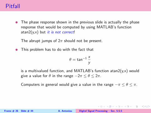
t The phase response shown in the previous slide is actually the phaseresponse that would be computed by using MATLAB’s functionatan2(y,x) but it is not correct!
The abrupt jumps of 2π should not be present.t This problem has to do with the fact that
θ = tan−1x
y
is a multivalued function, and MATLAB’s function atan2(y,x) wouldgive a value for θ in the range −2π ≤ θ ≤ 2π.
Computers in general would give a value in the range −π ≤ θ ≤ π.
t The problem can be corrected by noting that the phase response isa continuous function of ω.
Frame # 26 Slide # 44 A. Antoniou Digital Signal Processing – Sec. 5.5.5

Pitfall
t The phase response shown in the previous slide is actually the phaseresponse that would be computed by using MATLAB’s functionatan2(y,x) but it is not correct!
The abrupt jumps of 2π should not be present.t This problem has to do with the fact that
θ = tan−1x
y
is a multivalued function, and MATLAB’s function atan2(y,x) wouldgive a value for θ in the range −2π ≤ θ ≤ 2π.
Computers in general would give a value in the range −π ≤ θ ≤ π.t The problem can be corrected by noting that the phase response isa continuous function of ω.
Frame # 26 Slide # 45 A. Antoniou Digital Signal Processing – Sec. 5.5.5

Pitfall Cont’d
t For example, if function atan2(y,x) gives a value of −179followed by a value of +179◦ then, assuming a continuousphase response, an error of +360◦ has been committed and360◦ should be subtracted from +179◦ to give the correctvalue of −181◦.
t Similarly, if function atan2(y,x) gives a value of +179 followedby a value of −179◦, then an error of −360◦ has beencommitted and 360◦ should be added to −179◦ to give thecorrect value +181◦.t Alternatively, the correct value of the phase response can beobtained by using function unwrap(p) of MATLAB, which willperform the necessary corrections.
Frame # 27 Slide # 46 A. Antoniou Digital Signal Processing – Sec. 5.5.5
Pitfall Cont’d
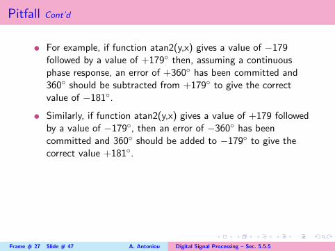
t For example, if function atan2(y,x) gives a value of −179followed by a value of +179◦ then, assuming a continuousphase response, an error of +360◦ has been committed and360◦ should be subtracted from +179◦ to give the correctvalue of −181◦.t Similarly, if function atan2(y,x) gives a value of +179 followedby a value of −179◦, then an error of −360◦ has beencommitted and 360◦ should be added to −179◦ to give thecorrect value +181◦.
t Alternatively, the correct value of the phase response can beobtained by using function unwrap(p) of MATLAB, which willperform the necessary corrections.
Frame # 27 Slide # 47 A. Antoniou Digital Signal Processing – Sec. 5.5.5

Pitfall Cont’d
t For example, if function atan2(y,x) gives a value of −179followed by a value of +179◦ then, assuming a continuousphase response, an error of +360◦ has been committed and360◦ should be subtracted from +179◦ to give the correctvalue of −181◦.t Similarly, if function atan2(y,x) gives a value of +179 followedby a value of −179◦, then an error of −360◦ has beencommitted and 360◦ should be added to −179◦ to give thecorrect value +181◦.t Alternatively, the correct value of the phase response can beobtained by using function unwrap(p) of MATLAB, which willperform the necessary corrections.
Frame # 27 Slide # 48 A. Antoniou Digital Signal Processing – Sec. 5.5.5

Lowpass Filter Cont’d
t Unwrapped phase response:
−10 −5 0
(i)
5 10−30
−25
−20
−15
−10
−5
0
5
Frequency, rad/s
Phas
e sh
ift,
rad
Frame # 28 Slide # 49 A. Antoniou Digital Signal Processing – Sec. 5.5.5

Example – Nonrecursive Lowpass Filter
The figure shows a nonrecursive filter:
A2
A2
A0
A1
A1
Y(z)X(z)
A0 = 0.3352, A1 = 0.2540, A2 = 0.0784
Frame # 29 Slide # 50 A. Antoniou Digital Signal Processing – Sec. 5.5.5
Example Cont’d
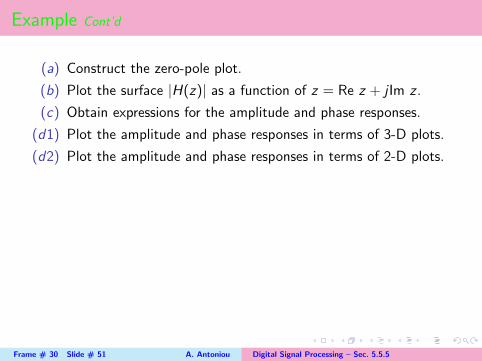
(a) Construct the zero-pole plot.
(b) Plot the surface |H(z)| as a function of z = Re z + j Im z .
(c) Obtain expressions for the amplitude and phase responses.
(d1) Plot the amplitude and phase responses in terms of 3-D plots.
(d2) Plot the amplitude and phase responses in terms of 2-D plots.
Frame # 30 Slide # 51 A. Antoniou Digital Signal Processing – Sec. 5.5.5

Example Cont’d
Solution
A2
A2
A0
A1
A1
Y(z)X(z)
Transfer function:
H(z) = A2 + A1z−1 + A0z
−2 + A1z−3 + A2z
−4
=A2z
2 + A1z + A0 + A1z−1 + A2z
−2
z2
=A2z
4 + A1z3 + A0z
2 + A1z + A2
z4
Frame # 31 Slide # 52 A. Antoniou Digital Signal Processing – Sec. 5.5.5

Example Cont’d
· · ·H(z) = A2 + A1z
−1 + A0z−2 + A1z
−3 + A2z−4
=A2z
2 + A1z + A0 + A1z−1 + A2z
−2
z2
=A2z
4 + A1z3 + A0z
2 + A1z + A2
z4
The zeros can be readily found by using D-Filter or MATLAB as
z1 = −1.5756 z2 = −0.6347 z3, z4 = −0.5148± j0.8573
There is a 4th-order pole at the origin.
Frame # 32 Slide # 53 A. Antoniou Digital Signal Processing – Sec. 5.5.5

Example Cont’d
Zero-pole plot:
−2 −1 0
(a)
1 2−2
−1
0
1
2
Re z
jIm
z
z1 = −1.5756 z2 = −0.6347 z3, z4 = −0.5148± j0.8573
p1 = p2 = p3 = p4 = 0
Frame # 33 Slide # 54 A. Antoniou Digital Signal Processing – Sec. 5.5.5

Example Cont’d
|H(z)| versus z = Re z + j Im z :
−50
0
50
100 |H
(z)|
, dB
Re z jIm z
−2
−1
0
1
2
−2
(b)
−1
0 1
2
Dimples represent zeros, the huge spike represents the 4th-order pole atthe origin.
Frame # 34 Slide # 55 A. Antoniou Digital Signal Processing – Sec. 5.5.5

Example Cont’d
Since
H(z) = A2 + A1z−1 + A0z
−2 + A1z−3 + A2z
−4
=A2z
2 + A1z + A0 + A1z−1 + A2z
−2
z2(A)
=A2z
4 + A1z3 + A0z
2 + A1z + A2
z4
Eq. (A) gives the frequency response as
H(e jωT ) =A2(e j2ωT + e−j2ωT ) + A1(e jωT + e−jωT ) + A0
e j2ωT
=2A2 cos 2ωT + 2A1 cosωT + A0
e j2ωT
Frame # 35 Slide # 56 A. Antoniou Digital Signal Processing – Sec. 5.5.5
Example Cont’d
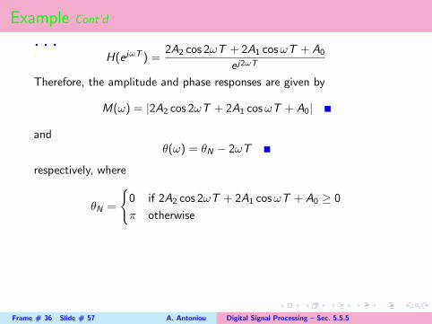
· · ·H(e jωT ) =
2A2 cos 2ωT + 2A1 cosωT + A0
e j2ωT
Therefore, the amplitude and phase responses are given by
M(ω) = |2A2 cos 2ωT + 2A1 cosωT + A0|
andθ(ω) = θN − 2ωT
respectively, where
θN =
{0 if 2A2 cos 2ωT + 2A1 cosωT + A0 ≥ 0
π otherwise
Note: The phase response is usually a linear function of ω innonrecursive filters (see Chap. 9).
Frame # 36 Slide # 57 A. Antoniou Digital Signal Processing – Sec. 5.5.5

Example Cont’d
· · ·H(e jωT ) =
2A2 cos 2ωT + 2A1 cosωT + A0
e j2ωT
Therefore, the amplitude and phase responses are given by
M(ω) = |2A2 cos 2ωT + 2A1 cosωT + A0|
andθ(ω) = θN − 2ωT
respectively, where
θN =
{0 if 2A2 cos 2ωT + 2A1 cosωT + A0 ≥ 0
π otherwise
Note: The phase response is usually a linear function of ω innonrecursive filters (see Chap. 9).
Frame # 36 Slide # 58 A. Antoniou Digital Signal Processing – Sec. 5.5.5

Example Cont’d
3-D plot of amplitude response, i.e., argH(e jωT ) versus z = e jωT :
−60
−50
−40
−30
−20
−10
0
Gain
, d
B
Re z jIm z
−2
−1
0
1
2
−2 −1
0
(c)
1 2
Frame # 37 Slide # 59 A. Antoniou Digital Signal Processing – Sec. 5.5.5

Example Cont’d
3-D plot of phase response, i.e., argH(e jωT ) versus z = e jωT :
−20
−15
−10
−5
0
5
Phase
shif
t, r
ad
Re z jIm z
−2
−1
0
(d)
1
2
−2
−1
0
1 2
Note: The phase angle has been unwrapped.
Frame # 38 Slide # 60 A. Antoniou Digital Signal Processing – Sec. 5.5.5

Example Cont’d
2-D plot of amplitude response, i.e., M(ω) = |H(e jωT )| versus ω:
−10 −5 0
(e)
5 10 −60
−50
−40
−30
−20
−10
0
Frequency, rad/s
Gai
n, dB
Frame # 39 Slide # 61 A. Antoniou Digital Signal Processing – Sec. 5.5.5

Example Cont’d
2-D plot of phase response, i.e., argH(e jωT ) versus ω:
−10 −5 0
( f )
5 10 −20
−15
−10
−5
0
5
Frequency, rad/s
Phas
e sh
ift,
rad
Note: The discontinuities are genuine: they are caused by zeros on theunit circle.
Frame # 40 Slide # 62 A. Antoniou Digital Signal Processing – Sec. 5.5.5

Example – Recursive Bandpass Filter
A recursive digital filter is characterized by the transfer function
H(z) = H0
3∏i=1
Hi (z)
where
Hi (z) =a0i + a1iz + z2
b0i + b1iz + z2
The sampling frequency is 20 rad/s.
Transfer-Function Coefficients
i a0i a1i b0i b1i
1 −1.0 0.0 8.131800E−1 7.870090E−82 1.0 −1.275258 9.211099E−1 5.484026E−13 1.0 1.275258 9.211097E−1 −5.484024E−1
H0 = 1.763161E − 2
Frame # 41 Slide # 63 A. Antoniou Digital Signal Processing – Sec. 5.5.5

Example Cont’d
(a) Construct the zero-pole plot of the filter.
(b) Plot the surface |H(z)| as a function of z = Re z + j Im z .
(c) Obtain expressions for the amplitude and phase responses.
(d) Plot the amplitude and phase responses first in terms of 3-Dplots and then in terms of 2-D plots.
Frame # 42 Slide # 64 A. Antoniou Digital Signal Processing – Sec. 5.5.5

Example Cont’d
Solution
−2 −1 0
(a)
1 2−2
−1
0
1
2
Re z
jIm
z
z1, z2 = ±1 z3, z4 = 0.638± j0.770 z5, z6 = −0.638± j0.770
p1, p2 = ±j0.902 p3, p4 = 0.274± j0.770 p5, p6 = −0.274± j0.770
Frame # 43 Slide # 65 A. Antoniou Digital Signal Processing – Sec. 5.5.5

Example Cont’d
|H(z)| versus z = Re z + j Im z :
−60
−40
−20
0
20
40
|H(z
) |, d
B
Re z jIm z
−2
−1
0
1
2
−2−1
0
(b)
12
Dimples represent zeros, the huge spike represents the 4th-order pole atthe origin.
Frame # 44 Slide # 66 A. Antoniou Digital Signal Processing – Sec. 5.5.5

Example Cont’d
Plot of |H(z)| (in dB) versus z = e jωT :
−60
−50
−40
−30
−20
−10
0
M(ω
), d
B
Re z jIm z
−2
−1
0
12
−2−1
0
(c)
12
The intersection between surface |H(z)| and the cylinder, i.e., thesolid curve, is the amplitude response.
Frame # 45 Slide # 67 A. Antoniou Digital Signal Processing – Sec. 5.5.5
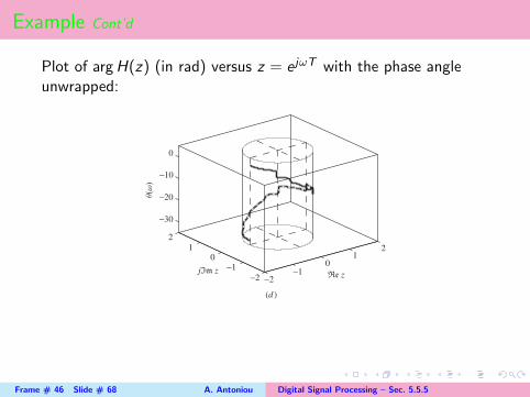
Example Cont’d
Plot of argH(z) (in rad) versus z = e jωT with the phase angleunwrapped:
−30
−20
−10
0θ(ω
)
Re z jIm z−2
−1
0
1
2
−2−1
01
2
(d )
Frame # 46 Slide # 68 A. Antoniou Digital Signal Processing – Sec. 5.5.5
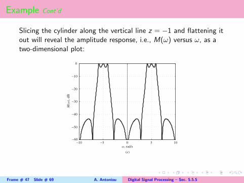
Example Cont’d
Slicing the cylinder along the vertical line z = −1 and flattening itout will reveal the amplitude response, i.e., M(ω) versus ω, as atwo-dimensional plot:
−10 −5 0
(e)
5 10−60
−50
−40
−30
−20
−10
0
ω, rad/s
M(ω
), d
B
Frame # 47 Slide # 69 A. Antoniou Digital Signal Processing – Sec. 5.5.5

Example Cont’d
Unwrapped phase response:
−10 −5 0
( f )
5 10−35
−30
−25
−20
−15
−10
−5
0
5
ω, rad/s
θ(ω
), r
ad
Note: The discontinuities shown are genuine. They are caused by thezeros on the unit circle.
Frame # 48 Slide # 70 A. Antoniou Digital Signal Processing – Sec. 5.5.5

This slide concludes the presentation.
Thank you for your attention.
Frame # 49 Slide # 71 A. Antoniou Digital Signal Processing – Sec. 5.5.5


![DSP, Z transform 1ce.sharif.edu/courses/93-94/1/ce763-2/resources/root/Lecture Notes... · ROC is necessary! To completely define a Z T, you must specify the ROC: z-plane x[n] x[n]](https://static.fdocuments.us/doc/165x107/6047d969fcd43f61906bd193/dsp-z-transform-1ce-notes-roc-is-necessary-to-completely-define-a-z-t-you.jpg)