Chapter 5 Syntax Trees

The parser we constructed in the last chapter can detect and report syntax errors, which is a

big, important job. When there is no syntax error, you need to build a data structure during

parsing that represents the whole program logically. This data structure is based on how the

different tokens and larger pieces of the program are grouped together. A syntax tree is a

tree data structure that records the branching structure of the grammar rules used by the

parsing algorithm to check the syntax of an input source file. A branch occurs whenever two

or more symbols were grouped together on the right-hand side of a grammar rule to build a

non-terminal symbol. This chapter will show you how to build syntax trees, which are the

central data structure for your programming language implementation.

This chapter covers the following main topics:

• Learning about trees

• Creating leaves from terminal symbols

• Building internal nodes from production rules

• Forming syntax trees for the Jzero language

• Debugging and testing your syntax tree

It is time to learn about tree data structures, and how to build them. But first, let’s learn

some new tools that will make building your language easier for the rest of this book.

Technical requirements

There are two tools for you to install for this chapter.

• Dot is part of a package called Graphviz that can be downloaded from a

downloads page found on http://graphviz.org. After successfully installing graphviz

you should have an executable named dot (or dot.exe) on your path.

• GNU make is a tool for helping manage large programming projects that supports

both Unicon and Java. It is available for Windows from

http://gnuwin32.sourceforge.net/packages/make.htm. Most programmers

probably get it along with their C/C++ compiler or with a development suite such as

MSYS2 or Cygwin. On Linux you typically get make from a C development suite

although it is often also a separate package you can install.

Before we dive into the main topics of this chapter, let’s explore the basics of how to use

GNU make and why you need it for developing your language.

Using GNU make

The command lines are growing longer and longer. You will get very tired typing the

commands required to build a programming language. We are already using Unicon, Java,

uflex, jflex, iyacc, and BYACC/J. Few tools for building large programs are multi-platform and

multi-language enough for this toolset. We will use the ultimate: GNU make.

Given a make program installed on your path, you can store the build rules for Unicon or

Java or both in a file named makefile, and then just run make whenever you have

changed the code and need to rebuild. A full treatment of make is beyond the scope of this

book, but here are the key points.

A makefile is like a lex or yacc specification, except instead of recognizing patterns of

strings, a makefile specifies a graph of build dependencies between files. For each file,

the makefile contains what source files it depends on as well as a list of one or more

command lines needed to build that file. The makefile header just consists of macros

defined by NAME= – strings that are used in later lines by writing $(NAME) to replace a

name with its – definition. The rest of the makefile lines are dependencies written in the

following format.

file: source_file(s)

build rule

In the first line, file is an output file you want to build, also called a target. The first line

specifies that the target depends on current versions of the source file(s). They are

required in order to make the target. The build rule is the command line that you

execute to make that output file from those source file(s).

Don’t forget the Tab!

The make program supports multiple lines of build rules, as long as the lines continue to

start with a tab. The most common newbie mistake in writing a makefile is that the build

rule line(s) must begin with an ASCII Control-I, also known as a tab character. Some text

editors will totally blow this. If your build rule lines don’t start with a tab, make will probably

give you some confusing error message. Use a real coder’s editor and don’t forget the tab.

The following example makefile will build both Unicon and Java if you just say make. If

you run make unicon or make java then it only builds one or the other. Added to the

commands from the last chapter is a new module (tree.icn or tree.java) for this

chapter. The makefile is presented in two halves, for the Unicon and then for the Java

build, respectively.

The target named all specifies what to build if make is invoked without an argument

saying what to build. The rest of the first half is concerned with building Unicon. The macros

U (and IYU for iyacc) list the Unicon modules that are separately compiled into a machine

code format called ucode. The strange dependency .icn.u: is called a suffix rule. It

says that all .u files are built from .icn files by running unicon -c on the .icn file. The

executable named j0 is built from the ucode files by running unicon on all the .u files to

link them together. The javalex.icn and j0gram.icn files are built using uflex and

iyacc, respectively. Let’s look at the first half of our makefile for this chapter.

all: unicon java

IYU=j0gram.u j0gram_tab.u

U=j0.u javalex.u token.u yyerror.u tree.u $(IYU)

unicon: j0

.icn.u:

unicon -c $<

j0: $(U)

unicon $(U)

javalex.icn: javalex.l

uflex javalex.l

j0gram.icn j0gram_tab.icn: j0gram.y

iyacc -dd j0gram.y

The Java build rules occupy the second half of our makefile. Macro JSRC gives the

names of all the Java files to be compiled. Macros BYSRC for BYACC/J-generated sources),

BYJOPTS for BYACC/J options, and IMP and BYJIMPS for BYACC/J static imports serve to

shorten later lines in the makefile so that they fit within this book’s formatting

constraints. Here is the second half of our makefile.

BYSRC=parser.java parserVal.java Yylex.java

JSRC=j0.java tree.java token.java yyerror.java $(BYSRC)

BYJOPTS= -Jclass=parser -Jpackage=ch5

IMP=importstatic

BYJIMPS= -J$(IMP)=ch5.j0.yylex -J$(IMP)=ch5.yyerror.yyerror

j: java

java ch5.j0 hello.java

dot -Tpng foo.dot >foo.png

java: j0.class

j0.class: $(JSRC)

javac $(JSRC)

parser.java parserVal.java: j0gram.y

yacc $(BYJOPTS) $(BYJIMPS) j0gram.y

Yylex.java: javalex.l

jflex javalex.l

In addition to the rules for compiling the Java code, the Java part of the makefile has an

artificial target make j that runs the compiler and invokes the dot program to generate a

PNG image of your syntax tree.

If makefiles are strange and scary-looking, don’t worry. You are in good company. This is a

red pill blue pill moment. You can close your eyes and just type make at the command line.

Or you can dig in and take ownership of this universal multi-language software development

build tool. If you want to read more about make, you might want to read GNU Make: A

Program for Directed Compilation, by Stallman and McGrath, or one of the other fine

books on make. Now it is time to get on with syntax trees, but first you have to know what a

tree is and how to define a tree data type for use in a programming language.

Learning about trees

Mathematically a tree is a kind of graph structure; it consists of nodes and edges that

connect those nodes. All the nodes in a tree are connected. A single node at the top is called

the root. Tree nodes can have zero or more children, and at most one parent. A tree node

with zero children is called a leaf; most trees have a lot of leaves. A tree that is not a leaf

has one or more children and is called an internal node. Figure 5.1 shows an example

tree with a root, two additional internal nodes, and five leaves.

Figure 5.1 – An illustration of a tree with root, internal nodes, and leaves

Trees have a property called arity that says what is the maximum number of children a

node can have. An arity of one would give you a linked list. Perhaps the most common kind

of trees are binary trees (arity = 2). The kind of trees we need have as many children as

there are symbols on the righthand sides of the rules in our grammar; these are so-called n-

ary trees. While there is no arity bound for arbitrary context free grammars, for any

grammar we can just look and see which production rule has the most symbols on its

righthand side, and code our tree arity to that number if needed. In j0gram.y from the

last chapter, the arity of Jzero is 9, although most non-leaf nodes will have two to four

children. In the following subsections, we will dive deeper and learn how to define syntax

trees and understand the difference between a parse tree and syntax tree.

Defining a syntax tree type

Every node in a tree has several pieces of information that need to be represented in the

class or data type used for tree nodes. This includes the following information:

• Labels or integer codes that uniquely identify the node and what kind of node it is.

• A data payload consisting of whatever information is associated with that node, and

• Information about that node’s children, including how many children it has and

references to those children (if any).

We use a class for this information in order to keep the mapping to Java as simple as

possible. Here is an outline of the tree class with its fields and constructor code; the

methods will be presented in the sections that follow within this chapter. The tree

information can be represented in Unicon in a file named tree.icn as follows.

class tree(id, label, rule, nkids, tok, kids)

initially(s,r,t[])

id := serial.getid()

label := s; rule := r

if type(t[1]) == "token" then tok := t[1]

else { kids := t; nkids := *t }

end

The tree class has the following fields.

• The field id is a unique integer identity, or serial number, that is used to distinguish

tree nodes from each other. It is initialized by calling a method getid() in a

singleton class named serial that will be presented later in this section.

• The string label is a human readable description for debugging purposes.

• The member named rule holds which production rule (or in the case of a leaf, the

integer category) the node represents. Yacc does not provide a numeric encoding

for production rules, so you will have to make your own, whether you just count

rules starting from 1 or get fancier. If you start at 1000, or use negative numbers,

you will never confuse a production rule number for a terminal symbol code.

• The member named nkids holds the number of child nodes underneath this node.

Usually it will be 0 indicating a leaf, or a number 2 or higher indicating an internal

node.

• The member named tok holds the lexical attributes of a leaf node, which comes to

us via the yylex() function setting the parser’s yylval variable, as discussed in

Chapter 3, Programming Language Design.

• The member named kids is an array of tree objects.

The corresponding Java code looks like the following class tree in a file named tree.java.

Its members match the fields in the Unicon tree class given previously.

package ch5;

class tree {

int id;

String label;

int rule;

int nkids;

token tok;

tree kids[];

The tree.java file continues with two constructors for the tree class: one for leaves,

which takes a token object as an argument, and one for internal nodes, which takes

children. These can be seen in the following code.

public tree(String s, int r, token t) {

id = serial.getid();

label = s; rule = r; tok = t; }

public tree(String s, int r, tree[] t) {

id = serial.getid();

sym = s; rule = r; nkids = t.length;

kids = t;

}

}

The previous pair of constructors initialize a tree’s fields in an obvious way. You may be

curious about the identification ids initialized from a serial class. They are used to give each

node a unique identity required by the tool that draws the syntax trees for us graphically at

the end of this chapter. Before we proceed with using these constructors, let’s consider two

different mindsets regarding the trees we are constructing.

Parse trees versus syntax trees

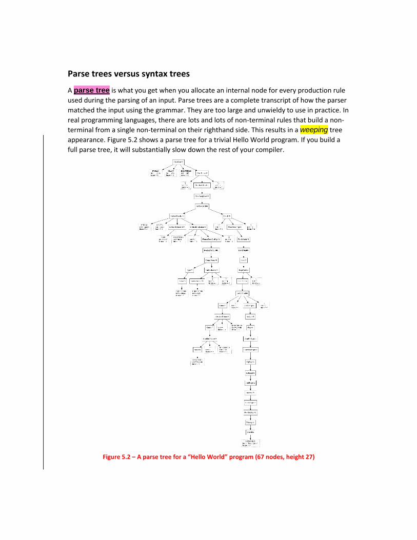
A parse tree is what you get when you allocate an internal node for every production rule

used during the parsing of an input. Parse trees are a complete transcript of how the parser

matched the input using the grammar. They are too large and unwieldy to use in practice. In

real programming languages, there are lots and lots of non-terminal rules that build a non-

terminal from a single non-terminal on their righthand side. This results in a weeping tree

appearance. Figure 5.2 shows a parse tree for a trivial Hello World program. If you build a

full parse tree, it will substantially slow down the rest of your compiler.

Figure 5.2 – A parse tree for a “Hello World” program (67 nodes, height 27)

A syntax tree is produced by allocating an internal node whenever a production rule has

two or more children on the righthand side that need representation in the tree. In that

case, the production rule needs a new node whenever the tree needs to branch out. The

easiest way to see the difference between a parse tree and a syntax tree is to look at an

example. Figure 5.3 shows a syntax tree for the hello.java program. Note the

differences in size and shape compared with the parse tree shown in Figure 5.2. This is why

we build syntax trees and not parse trees.

Figure 5.3 – A syntax tree for a “Hello World” program (20 nodes, height 8)

While a parse tree may be useful for studying or debugging a parsing algorithm, a

programming language implementation uses a much simpler tree. You will see this

especially when we present the rules for building tree nodes for our example language, in

the Forming syntax trees for the Jzero language section.

Creating leaves from terminal symbols

Leaves make up a large percentage of the nodes in a syntax tree. The leaves in a syntax

tree built by yacc come from the lexical analyzer. For this reason, this section discusses

modifications to the code from Chapter 3, Programming Language Design. After you

create leaves in the lexical analyzer, the parsing algorithm must pick them up somehow and

plug them into the tree that it builds. This section describes that process in detail. First you

will learn how to embed token structures into tree leaves, then you will learn how these

leaves are picked up by the parser in its value stack. For Java, you will need to know about

an extra type that is needed to work with the value stack. Lastly, the section provides some

guidance as to which leaves are really necessary and which can be safely omitted. Here is

how to create the leaves containing token information.

Wrapping tokens in leaves

The tree type presented earlier contains a field that is a reference to the token type

introduced in Chapter 3, Programming Language Design. Every leaf will get a

corresponding token and vice versa. Think of this as wrapping up the token inside a tree

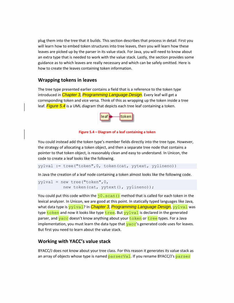
leaf. Figure 5.4 is a UML diagram that depicts each tree leaf containing a token.

Figure 5.4 – Diagram of a leaf containing a token

You could instead add the token type’s member fields directly into the tree type. However,

the strategy of allocating a token object, and then a separate tree node that contains a

pointer to that token object, is reasonably clean and easy to understand. In Unicon, the

code to create a leaf looks like the following.

yylval := tree("token",0, token(cat, yytext, yylineno))

In Java the creation of a leaf node containing a token almost looks like the following code.

yylval = new tree("token",0,

new token(cat, yytext(), yylineno));

You could put this code within the j0.scan() method that is called for each token in the

lexical analyzer. In Unicon, we are good at this point. In statically typed languages like Java,

what data type is yylval? In Chapter 3, Programming Language Design, yylval was

type token and now it looks like type tree. But yylval is declared in the generated

parser, and yacc doesn’t know anything about your token or tree types. For a Java

implementation, you must learn the data type that yacc’s generated code uses for leaves.

But first you need to learn about the value stack.

Working with YACC’s value stack

BYACC/J does not know about your tree class. For this reason it generates its value stack as

an array of objects whose type is named parserVal. If you rename BYACC/J’s parser

class to something else like myparse using the -Jclass= command line option, the value

stack class will also automatically be renamed, to myparseVal.

Variable yylval is part of yacc’s public interface. Every time yacc shifts the next

terminal symbol onto its parse stack, it copies the contents of yylval onto a stack that it

manages in parallel with the parse stack, called the value stack. BYACC/J declares the

value stack elements as well as yylval in the parser class to be of a type parserVal.

Since the parse stack is managed in parallel with the value stack, whenever a new state is

pushed on the parse stack, the value stack sees a corresponding push; the same goes for

pop operations. Value stack entries whose parse state was produced by a shift operation

hold tree leaves. Value stack entries whose parse state was produced by a reduce operation

hold internal syntax tree nodes. Figure 5.5 depicts the value stack in parallel with the parse

stack.

Figure 5.5 – The parse stack and the value stack

In Figure 5.5, the $ on the left edge represents the bottom of the two stacks, which grow

towards the right when values are pushed on the stack. The right side of the figure depicts

the sequence of terminal symbols whose tokens are produced by lexical analysis. Tokens are

processed from left to right, with the $ at the right edge of the screen representing end of

file, also depicted as EOF. The ellipses (…) on the left side represent the room on the two

stacks to process additional push operations during parsing, while those on the right side

represent whatever additional input symbols remain after those that are depicted.

The parserVal type was briefly mentioned in Chapter 4, Parsing. To build syntax trees

in BYACC/J we must go into it in detail. Here is the parserVal type as defined by BYACC/J.

public class parserVal {

public int ival;

public double dval;

public String sval;

public Object obj;

public parserVal() { }

public parserVal(int val){ ival=val; }

public parserVal(double val) { dval=val; }

public parserVal(String val) { sval=val; }

public parserVal(Object val) { obj=val; }

}

A parserVal is a container that holds an int, a double, a String, and an Object,

which can be a reference to any class instance at all. Having four fields here is a waste of

memory for us since we will only use the obj field, but yacc is a generic tool. In any case,

let’s look at wrapping tree leaves within a parserVal object in order to place them in

yylval.

Wrapping leaves for the parser’s value stack

In terms of mechanics, parserVal is a third data type in the code that builds our syntax

tree. BYACC/J requires that we use this type for the lexical analyzer to communicate tokens

to the parser. For this reason, for the Java implementation, this chapter’s class j0’s

scan() method looks like the following code.

public static int scan(int cat) {

ch5.j0.par.yylval =

new parserVal(

new tree("token",0,

new token(cat, yytext(), yylineno)));

return cat;

}

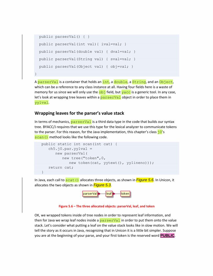
In Java, each call to scat() allocates three objects, as shown in Figure 5.6. In Unicon, it

allocates the two objects as shown in Figure 5.3.

Figure 5.6 – The three allocated objects: parserVal, leaf, and token

OK, we wrapped tokens inside of tree nodes in order to represent leaf information, and

then for Java we wrap leaf nodes inside a parserVal in order to put them onto the value

stack. Let’s consider what putting a leaf on the value stack looks like in slow motion. We will

tell the story as it occurs in Java, recognizing that in Unicon it is a little bit simpler. Suppose

you are at the beginning of your parse, and your first token is the reserved word PUBLIC.

The scenario is shown in Figure 5.7. See the description of Figure 5.5 if you need a

refresher on how this figure is organized.

Figure 5.7 – The parse stack state at the start of parsing

The first operation is a shift. An integer finite automation state that encodes the fact that

we saw PUBLIC is pushed onto the stack. yylex() calls scan() which allocates a leaf

wrapped in a parserVal and assigns yylval a reference to it, which yylex() pushes

onto the value stack. The stacks are in lock-step as shown in Figure 5.8.

Figure 5.8 – The parse and value stack state after a shift operation

Another of these wrapped leaves gets added to the value stack each time a shift occurs.

Now it is time to consider how all these leaves get placed into the internal nodes, and how

internal nodes get assembled into higher level nodes, until you get back to the root. This all

happens one node at a time, when a production rule in the grammar is matched.

Determining which leaves you need

In most languages, punctuation marks like semi-colons and parentheses are only necessary

up through syntax analysis. Maybe they help for human readability, or force operator

precedence, or make the grammar parse unambiguously. Once you successfully parse the

input, you will never again need those leaves in your syntax tree for subsequent semantic

analysis or code generation.

You can omit unnecessary leaves from the tree, or you can leave them in so that their

source line number and filename information is in the tree in case it is needed for error

message reporting. I usually omit them by default but add in specific punctuation leaves if I

determine that they are needed for some reason.

The flipside of this equation is: any leaf that contains a value or a name or other semantic

meaning of some kind in the language needs to be kept around in the syntax tree. This

includes literal constants, identifiers, and other reserved words or operators. Now let’s look

at how and when to build internal nodes for your syntax tree.

Building internal nodes from production rules

In this section, we will learn how to construct the tree, one node at a time, during parsing.

The internal nodes of your syntax tree, all the way back up to the root, are built from the

bottom up, following the sequence of reduce operations with which production rules are

recognized during the parse. The tree nodes used during the construction are accessed from

the value stack.

Accessing tree nodes on the value stack

For every production rule in the grammar, there is a chance to execute some code called a

semantic action when that production rule is used during a parse. As you saw in in

Chapter 4, Parsing in the Putting together the yacc context free grammar section,

semantic action code comes at the end of a grammar rule, before the semi-colon or vertical

bar that ends the rule and starts the next one.

You can put any code you want in a semantic action. For us the main purpose of a semantic

action is to build a syntax tree node. Use the value stack entries corresponding to the right

side of the production rule to construct the tree node for the symbol on the left side of the

production rule. The left side non-terminal that has been matched gets a new entry pushed

into the value stack that can hold the newly constructed tree node.

For this purpose, yacc provides macros that refer to each position on the value stack during

a reduce. $1, $2, … $N refer to the current value stack contents corresponding to the

grammar rule’s right hand symbols 1 through N. By the time the semantic action code

executes, these symbols have already been matched at some point in the recent past. They

are the top N symbols on the value stack, and during the reduce operation they will be

popped, and a new value stack entry pushed in their place. The new value stack entry is

whatever you assign to $$. By default, it will just be whatever is in $1; yacc’s default

semantic action is $$=$1 and that semantic action is correct for production rules with one

symbol (terminal or non-terminal) that is being reduced to the non-terminal on the left

hand side of the rule.

All of this is a lot to unpack. Here is a specific example.

Suppose you are just finishing up parsing the hello.java input

shown earlier, and where it is at the point where it is time

to reduce the reserved words PUBLIC, CLASS, the class name,

and the class body. The grammar rule that applies at this

point is the rule ClassDecl: PUBLIC CLASS IDENTIFIER ClassBody

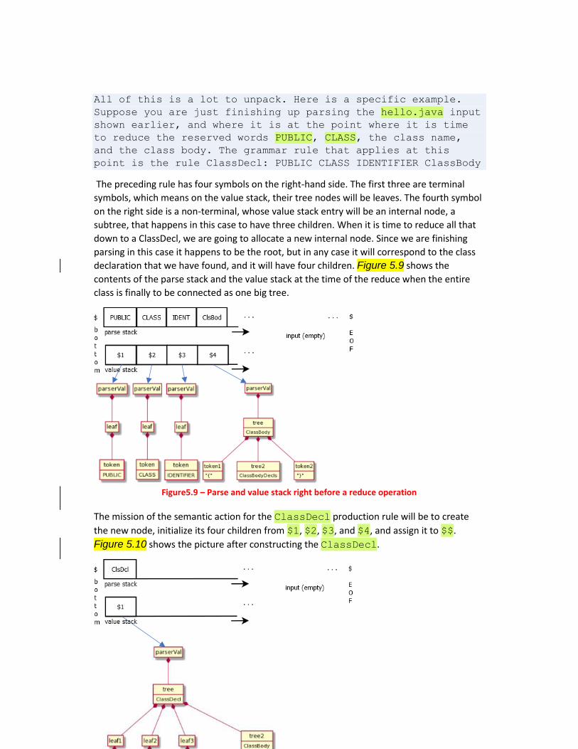
The preceding rule has four symbols on the right-hand side. The first three are terminal

symbols, which means on the value stack, their tree nodes will be leaves. The fourth symbol

on the right side is a non-terminal, whose value stack entry will be an internal node, a

subtree, that happens in this case to have three children. When it is time to reduce all that

down to a ClassDecl, we are going to allocate a new internal node. Since we are finishing

parsing in this case it happens to be the root, but in any case it will correspond to the class

declaration that we have found, and it will have four children. Figure 5.9 shows the

contents of the parse stack and the value stack at the time of the reduce when the entire

class is finally to be connected as one big tree.

Figure5.9 – Parse and value stack right before a reduce operation

The mission of the semantic action for the ClassDecl production rule will be to create

the new node, initialize its four children from $1, $2, $3, and $4, and assign it to $$.

Figure 5.10 shows the picture after constructing the ClassDecl.

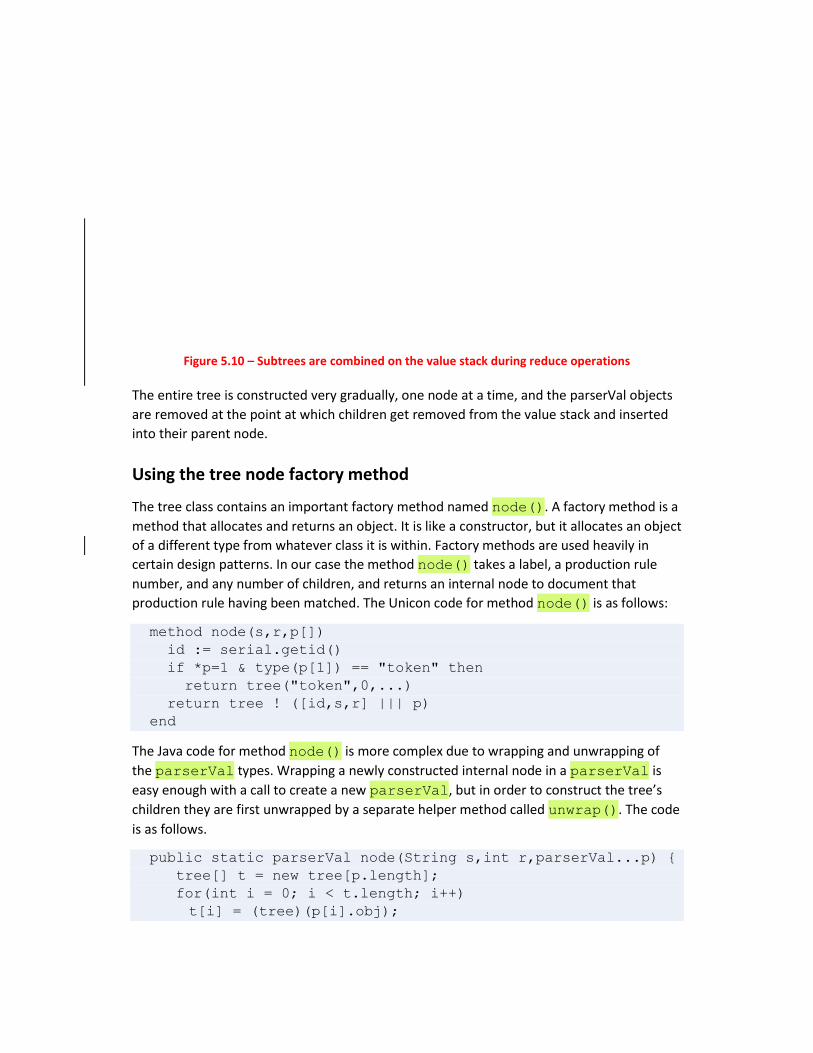
Figure 5.10 – Subtrees are combined on the value stack during reduce operations

The entire tree is constructed very gradually, one node at a time, and the parserVal objects

are removed at the point at which children get removed from the value stack and inserted

into their parent node.

Using the tree node factory method

The tree class contains an important factory method named node(). A factory method is a

method that allocates and returns an object. It is like a constructor, but it allocates an object

of a different type from whatever class it is within. Factory methods are used heavily in

certain design patterns. In our case the method node() takes a label, a production rule

number, and any number of children, and returns an internal node to document that

production rule having been matched. The Unicon code for method node() is as follows:

method node(s,r,p[])

id := serial.getid()

if *p=1 & type(p[1]) == "token" then

return tree("token",0,...)

return tree ! ([id,s,r] ||| p)

end

The Java code for method node() is more complex due to wrapping and unwrapping of

the parserVal types. Wrapping a newly constructed internal node in a parserVal is

easy enough with a call to create a new parserVal, but in order to construct the tree’s

children they are first unwrapped by a separate helper method called unwrap(). The code

is as follows.

public static parserVal node(String s,int r,parserVal...p) {

tree[] t = new tree[p.length];

for(int i = 0; i < t.length; i++)

t[i] = (tree)(p[i].obj);

return new parserVal((Object)new tree(s,r,t));

}

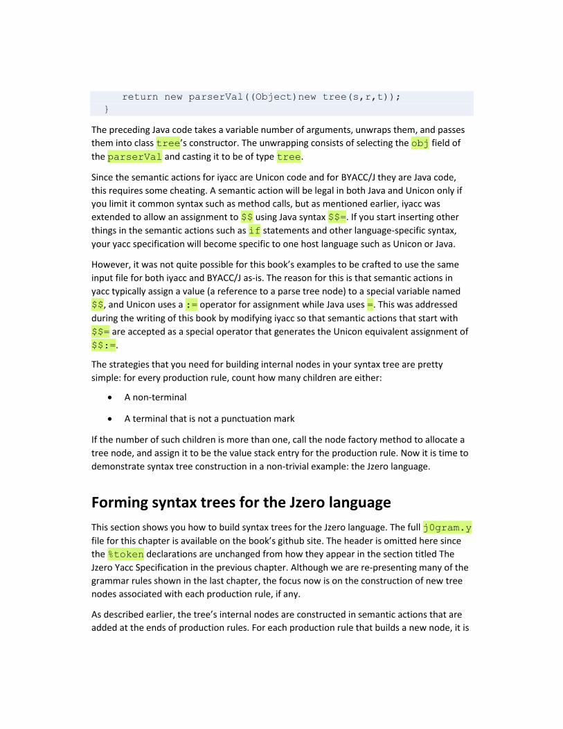
The preceding Java code takes a variable number of arguments, unwraps them, and passes

them into class tree’s constructor. The unwrapping consists of selecting the obj field of

the parserVal and casting it to be of type tree.

Since the semantic actions for iyacc are Unicon code and for BYACC/J they are Java code,

this requires some cheating. A semantic action will be legal in both Java and Unicon only if

you limit it common syntax such as method calls, but as mentioned earlier, iyacc was

extended to allow an assignment to $$ using Java syntax $$=. If you start inserting other

things in the semantic actions such as if statements and other language-specific syntax,

your yacc specification will become specific to one host language such as Unicon or Java.

However, it was not quite possible for this book’s examples to be crafted to use the same

input file for both iyacc and BYACC/J as-is. The reason for this is that semantic actions in

yacc typically assign a value (a reference to a parse tree node) to a special variable named

$$, and Unicon uses a := operator for assignment while Java uses =. This was addressed

during the writing of this book by modifying iyacc so that semantic actions that start with

$$= are accepted as a special operator that generates the Unicon equivalent assignment of

$$:=.

The strategies that you need for building internal nodes in your syntax tree are pretty

simple: for every production rule, count how many children are either:

• A non-terminal

• A terminal that is not a punctuation mark

If the number of such children is more than one, call the node factory method to allocate a

tree node, and assign it to be the value stack entry for the production rule. Now it is time to

demonstrate syntax tree construction in a non-trivial example: the Jzero language.

Forming syntax trees for the Jzero language

This section shows you how to build syntax trees for the Jzero language. The full j0gram.y

file for this chapter is available on the book’s github site. The header is omitted here since

the %token declarations are unchanged from how they appear in the section titled The

Jzero Yacc Specification in the previous chapter. Although we are re-presenting many of the

grammar rules shown in the last chapter, the focus now is on the construction of new tree

nodes associated with each production rule, if any.

As described earlier, the tree’s internal nodes are constructed in semantic actions that are

added at the ends of production rules. For each production rule that builds a new node, it is

assigned to $$, the yacc value corresponding to the new non-terminal symbol built by that

production rule.

The starting non-terminal, which in the case of Jzero is a single class declaration, is the point

at which the root of the entire tree is constructed. Its semantic action has extra work after

assigning the constructed node to $$. At this top level, in this chapter the code prints out

the tree by calling method print() in order to allow you to check if it is correct.

Subsequent chapters may assign the topmost tree node to a global variable named root

for subsequent processing or call a different method here to translate the tree to machine

code, or to execute the program directly by interpreting the statements in the tree.

%%

ClassDecl: PUBLIC CLASS IDENTIFIER ClassBody {

$$=j0.node("ClassDecl",1000,$3,$4);

j0.print($$);

} ;

Non-terminal ClassBody either contains declarations (first production rule) or is empty.

In the empty case, it is an interesting question whether to assign an explicit leaf node

indicating an empty ClassBody as is done here, or whether the code should just say

$$=null.

ClassBody: '{' ClassBodyDecls '}' {

$$=j0.node("ClassBody",1010,$2); }

| '{' '}' { $$=j0.node("ClassBody",1011); };

Non-terminal ClassBodyDecls chains together as many fields, methods, and

constructors as appear within the class. The first production rule terminates the recursions

in the second production rule with a single ClassBodyDecl. Since there is no semantic action

in the first production rule it executes $$=$1; the subtree for the ClassBodyDecl is

promoted instead of creating a node for the parent.

ClassBodyDecls: ClassBodyDecl

| ClassBodyDecls ClassBodyDecl {

$$=j0.node("ClassBodyDecls",1020,$1,$2); };

There are three kinds of ClassBodyDecl to choose from. No extra tree node is allocated at

this level as it can be inferred which kind of ClassBodyDecl each subtree is.

ClassBodyDecl: FieldDecl | MethodDecl | ConstructorDecl ;

A field, or member variable, is declared with a base type followed by a list of variable

declarations.

FieldDecl: Type VarDecls ';' {

$$=j0.node("FieldDecl",1030,$1,$2); };

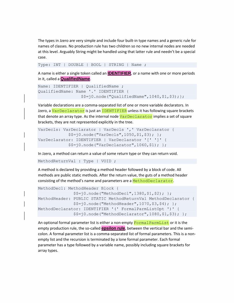
The types in Jzero are very simple and include four built-in type names and a generic rule for

names of classes. No production rule has two children so no new internal nodes are needed

at this level. Arguably String might be handled using that latter rule and needn’t be a special

case.

Type: INT | DOUBLE | BOOL | STRING | Name ;

A name is either a single token called an IDENTIFIER, or a name with one or more periods

in it, called a QualifiedName.

Name: IDENTIFIER | QualifiedName ;

QualifiedName: Name '.' IDENTIFIER {

$$=j0.node("QualifiedName",1040,$1,$3);};

Variable declarations are a comma-separated list of one or more variable declarators. In

Jzero, a VarDeclarator is just an IDENTIFIER unless it has following square brackets

that denote an array type. As the internal node VarDeclarator implies a set of square

brackets, they are not represented explicitly in the tree.

VarDecls: VarDeclarator | VarDecls ',' VarDeclarator {

$$=j0.node("VarDecls",1050,$1,$3); };

VarDeclarator: IDENTIFIER | VarDeclarator '[' ']' {

$$=j0.node("VarDeclarator",1060,$1); };

In Jzero, a method can return a value of some return type or they can return void.

MethodReturnVal : Type | VOID ;

A method is declared by providing a method header followed by a block of code. All

methods are public static methods. After the return value, the guts of a method header

consisting of the method’s name and parameters are a MethodDeclarator.

MethodDecl: MethodHeader Block {

$$=j0.node("MethodDecl",1380,$1,$2); };

MethodHeader: PUBLIC STATIC MethodReturnVal MethodDeclarator {

$$=j0.node("MethodHeader",1070,$3,$4); };

MethodDeclarator: IDENTIFIER '(' FormalParmListOpt ')' {

$$=j0.node("MethodDeclarator",1080,$1,$3); };

An optional formal parameter list is either a non-empty FormalParmList or it is the

empty production rule, the so-called epsilon rule, between the vertical bar and the semi-

colon. A formal parameter list is a comma-separated list of formal parameters. This is a non-

empty list and the recursion is terminated by a lone formal parameter. Each formal

parameter has a type followed by a variable name, possibly including square brackets for

array types.

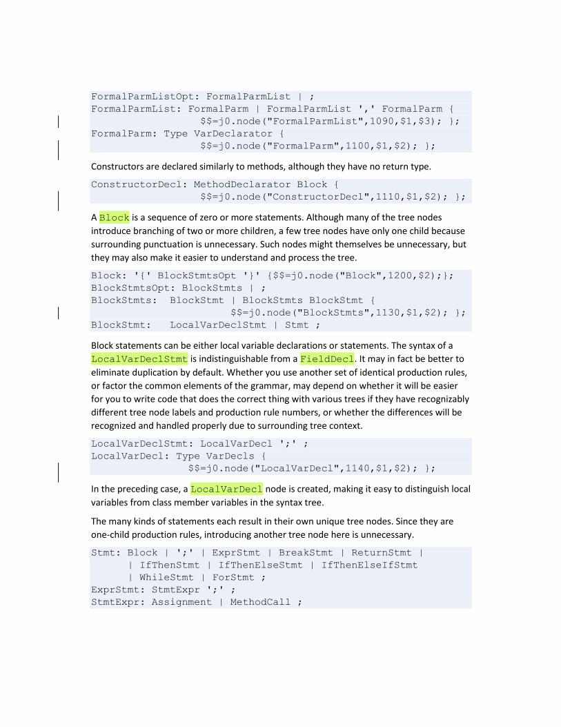
FormalParmListOpt: FormalParmList | ;

FormalParmList: FormalParm | FormalParmList ',' FormalParm {

$$=j0.node("FormalParmList",1090,$1,$3); };

FormalParm: Type VarDeclarator {

$$=j0.node("FormalParm",1100,$1,$2); };

Constructors are declared similarly to methods, although they have no return type.

ConstructorDecl: MethodDeclarator Block {

$$=j0.node("ConstructorDecl",1110,$1,$2); };

A Block is a sequence of zero or more statements. Although many of the tree nodes

introduce branching of two or more children, a few tree nodes have only one child because

surrounding punctuation is unnecessary. Such nodes might themselves be unnecessary, but

they may also make it easier to understand and process the tree.

Block: '{' BlockStmtsOpt '}' {$$=j0.node("Block",1200,$2);};

BlockStmtsOpt: BlockStmts | ;

BlockStmts: BlockStmt | BlockStmts BlockStmt {

$$=j0.node("BlockStmts",1130,$1,$2); };

BlockStmt: LocalVarDeclStmt | Stmt ;

Block statements can be either local variable declarations or statements. The syntax of a

LocalVarDeclStmt is indistinguishable from a FieldDecl. It may in fact be better to

eliminate duplication by default. Whether you use another set of identical production rules,

or factor the common elements of the grammar, may depend on whether it will be easier

for you to write code that does the correct thing with various trees if they have recognizably

different tree node labels and production rule numbers, or whether the differences will be

recognized and handled properly due to surrounding tree context.

LocalVarDeclStmt: LocalVarDecl ';' ;

LocalVarDecl: Type VarDecls {

$$=j0.node("LocalVarDecl",1140,$1,$2); };

In the preceding case, a LocalVarDecl node is created, making it easy to distinguish local

variables from class member variables in the syntax tree.

The many kinds of statements each result in their own unique tree nodes. Since they are

one-child production rules, introducing another tree node here is unnecessary.

Stmt: Block | ';' | ExprStmt | BreakStmt | ReturnStmt |

| IfThenStmt | IfThenElseStmt | IfThenElseIfStmt

| WhileStmt | ForStmt ;

ExprStmt: StmtExpr ';' ;

StmtExpr: Assignment | MethodCall ;

Several non-terminals in Jzero exist in order to allow common variations of if statements.

Blocks are required for bodies of conditionals and loops in Jzero in order to avoid a common

ambiguity when they are nested.

IfThenStmt: IF '(' Expr ')' Block {

$$=j0.node("IfThenStmt",1150,$3,$5); };

IfThenElseStmt: IF '(' Expr ')' Block ELSE Block {

$$=j0.node("IfThenElseStmt",1160,$3,$5,$7); };

IfThenElseIfStmt: IF '(' Expr ')' Block ElseIfSequence {

$$=j0.node("IfThenElseIfStmt",1170,$3,$5,$6); }

| IF '(' Expr ')' Block ElseIfSequence ELSE Block {

$$=j0.node("IfThenElseIfStmt",1171,$3,$5,$6,$8); };

ElseIfSequence: ElseIfStmt | ElseIfSequence ElseIfStmt {

$$=j0.node("ElseIfSequence",1180,$1,$2); };

ElseIfStmt: ELSE IfThenStmt {

$$=j0.node("ElseIfStmt",1190,$2); };

Tree nodes are generally created for these control structures, and they generally introduce

branching into the tree. Although while loops introduce only a single branch, the node for a

for loop has four children. Did language designers do that on purpose?

WhileStmt: WHILE '(' Expr ')' Stmt {

$$=j0.node("WhileStmt",1210,$3,$5); };

ForStmt: FOR '(' ForInit ';' ExprOpt ';' ForUpdate ')' Block {

$$=j0.node("ForStmt",1220,$3,$5,$7,$9); };

ForInit: StmtExprList | LocalVarDecl | ;

ExprOpt: Expr | ;

ForUpdate: StmtExprList | ;

StmtExprList: StmtExpr | StmtExprList ',' StmtExpr {

$$=j0.node("StmtExprList",1230,$1,$3); };

A break statement is adequately represented by the leaf that says BREAK.

BreakStmt: BREAK ';' ;

ReturnStmt: RETURN ExprOpt ';' {

$$=j0.node("ReturnStmt",1250,$2); };

A return statement needs a new node, since it is followed by an optional expression.

Primary expressions, including literals, do not introduce an additional layer of tree nodes

above the content of their child. The only interesting action here is for parenthesized

expressions, which discard the parentheses that were used for operator precedence and

promote the second child without need for an additional tree node at this level.

Primary: Literal | FieldAccess | MethodCall |

'(' Expr ')' { $$=$2; };

Literal: INTLIT | DOUBLELIT | BOOLLIT | STRINGLIT | NULLVAL ;

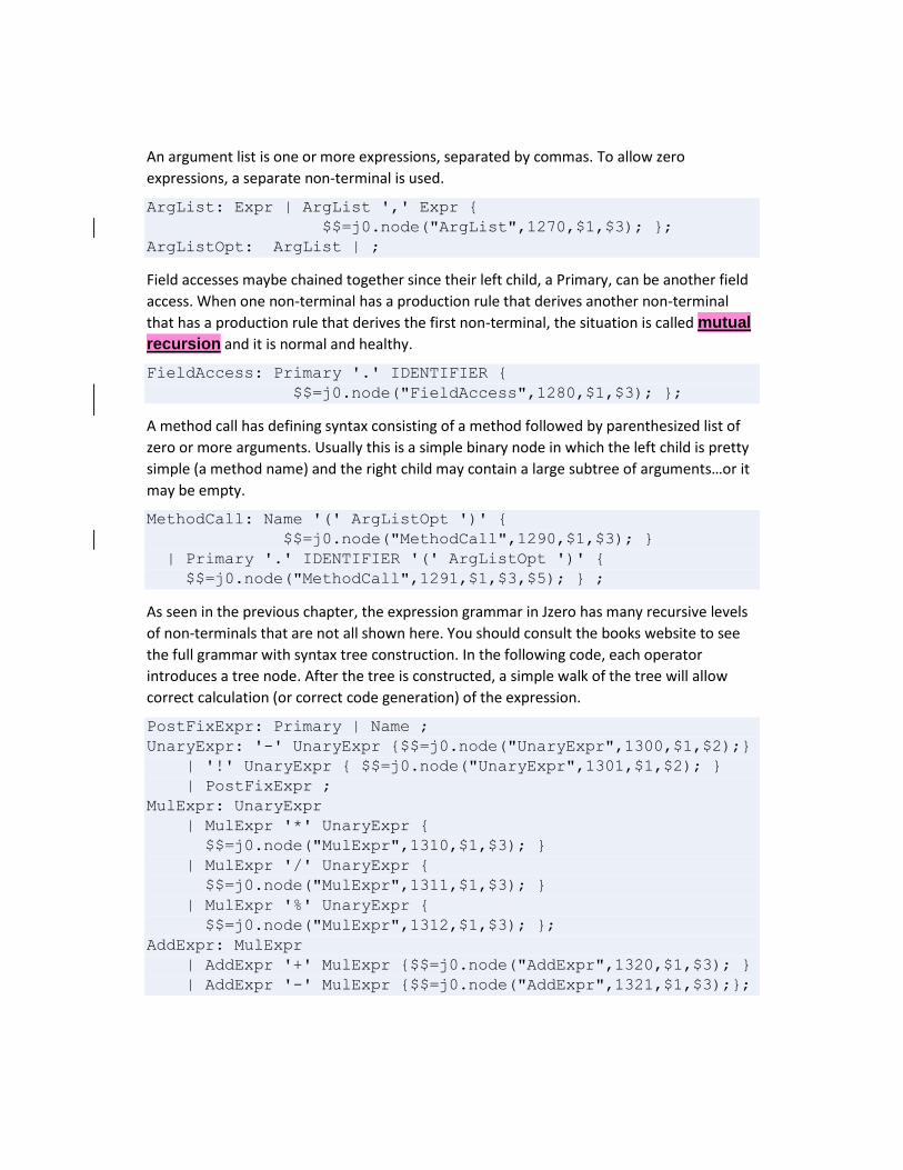
An argument list is one or more expressions, separated by commas. To allow zero

expressions, a separate non-terminal is used.

ArgList: Expr | ArgList ',' Expr {

$$=j0.node("ArgList",1270,$1,$3); };

ArgListOpt: ArgList | ;

Field accesses maybe chained together since their left child, a Primary, can be another field

access. When one non-terminal has a production rule that derives another non-terminal

that has a production rule that derives the first non-terminal, the situation is called mutual

recursion and it is normal and healthy.

FieldAccess: Primary '.' IDENTIFIER {

$$=j0.node("FieldAccess",1280,$1,$3); };

A method call has defining syntax consisting of a method followed by parenthesized list of

zero or more arguments. Usually this is a simple binary node in which the left child is pretty

simple (a method name) and the right child may contain a large subtree of arguments…or it

may be empty.

MethodCall: Name '(' ArgListOpt ')' {

$$=j0.node("MethodCall",1290,$1,$3); }

| Primary '.' IDENTIFIER '(' ArgListOpt ')' {

$$=j0.node("MethodCall",1291,$1,$3,$5); } ;

As seen in the previous chapter, the expression grammar in Jzero has many recursive levels

of non-terminals that are not all shown here. You should consult the books website to see

the full grammar with syntax tree construction. In the following code, each operator

introduces a tree node. After the tree is constructed, a simple walk of the tree will allow

correct calculation (or correct code generation) of the expression.

PostFixExpr: Primary | Name ;

UnaryExpr: '-' UnaryExpr {$$=j0.node("UnaryExpr",1300,$1,$2);}

| '!' UnaryExpr { $$=j0.node("UnaryExpr",1301,$1,$2); }

| PostFixExpr ;

MulExpr: UnaryExpr

| MulExpr '*' UnaryExpr {

$$=j0.node("MulExpr",1310,$1,$3); }

| MulExpr '/' UnaryExpr {

$$=j0.node("MulExpr",1311,$1,$3); }

| MulExpr '%' UnaryExpr {

$$=j0.node("MulExpr",1312,$1,$3); };

AddExpr: MulExpr

| AddExpr '+' MulExpr {$$=j0.node("AddExpr",1320,$1,$3); }

| AddExpr '-' MulExpr {$$=j0.node("AddExpr",1321,$1,$3);};

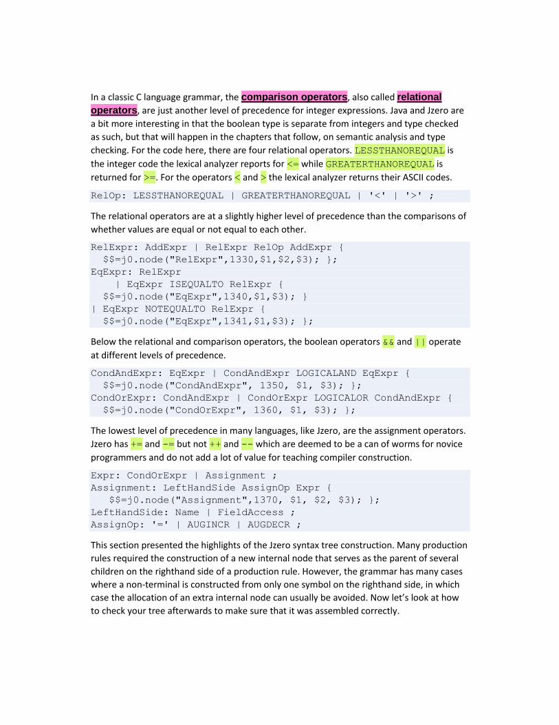
In a classic C language grammar, the comparison operators, also called relational

operators, are just another level of precedence for integer expressions. Java and Jzero are

a bit more interesting in that the boolean type is separate from integers and type checked

as such, but that will happen in the chapters that follow, on semantic analysis and type

checking. For the code here, there are four relational operators. LESSTHANOREQUAL is

the integer code the lexical analyzer reports for <= while GREATERTHANOREQUAL is

returned for >=. For the operators < and > the lexical analyzer returns their ASCII codes.

RelOp: LESSTHANOREQUAL | GREATERTHANOREQUAL | '<' | '>' ;

The relational operators are at a slightly higher level of precedence than the comparisons of

whether values are equal or not equal to each other.

RelExpr: AddExpr | RelExpr RelOp AddExpr {

$$=j0.node("RelExpr",1330,$1,$2,$3); };

EqExpr: RelExpr

| EqExpr ISEQUALTO RelExpr {

$$=j0.node("EqExpr",1340,$1,$3); }

| EqExpr NOTEQUALTO RelExpr {

$$=j0.node("EqExpr",1341,$1,$3); };

Below the relational and comparison operators, the boolean operators && and || operate

at different levels of precedence.

CondAndExpr: EqExpr | CondAndExpr LOGICALAND EqExpr {

$$=j0.node("CondAndExpr", 1350, $1, $3); };

CondOrExpr: CondAndExpr | CondOrExpr LOGICALOR CondAndExpr {

$$=j0.node("CondOrExpr", 1360, $1, $3); };

The lowest level of precedence in many languages, like Jzero, are the assignment operators.

Jzero has += and -= but not ++ and -- which are deemed to be a can of worms for novice

programmers and do not add a lot of value for teaching compiler construction.

Expr: CondOrExpr | Assignment ;

Assignment: LeftHandSide AssignOp Expr {

$$=j0.node("Assignment",1370, $1, $2, $3); };

LeftHandSide: Name | FieldAccess ;

AssignOp: '=' | AUGINCR | AUGDECR ;

This section presented the highlights of the Jzero syntax tree construction. Many production

rules required the construction of a new internal node that serves as the parent of several

children on the righthand side of a production rule. However, the grammar has many cases

where a non-terminal is constructed from only one symbol on the righthand side, in which

case the allocation of an extra internal node can usually be avoided. Now let’s look at how

to check your tree afterwards to make sure that it was assembled correctly.

Debugging and testing your syntax tree

The trees that you build must be rock solid. What this spectacular mixed metaphor means

is: if your syntax tree structure is not built correctly, you can’t expect to be able to build the

rest of your programming language. The most direct way of testing that the tree has been

constructed correctly is to walk back through it and look at the tree that you have built. This

section contains two examples of doing that. You will print your tree first in a human

readable (more or less) ASCII text format, then you will learn how to print it out in a format

that is easily rendered graphically using the popular open source Graphviz package,

commonly accessed through PlantUML or the classic command line tool called dot. First,

consider some of the most common causes of problems in syntax trees.

Avoiding common syntax tree bugs

The most common problems with syntax trees result in program crashes when you print the

tree out. Each tree node may hold references (pointers) to other objects, and when these

references are not initialized correctly: boom! Debugging problems with references is

difficult, even in higher level languages.

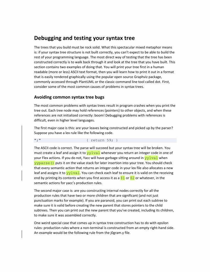
The first major case is this: are your leaves being constructed and picked up by the parser?

Suppose you have a lex rule like the following code.

";" { return 59; }

The ASCII code is correct. The parse will succeed but your syntax tree will be broken. You

must create a leaf and assign it to yylval whenever you return an integer code in one of

your Flex actions. If you do not, Yacc will have garbage sitting around in yylval when

yyparse() puts it on the value stack for later insertion into your tree. You should check

that every semantic action that returns an integer code in your lex file also allocates a new

leaf and assigns it to yylval. You can check each leaf to ensure it is valid on the receiving

end by printing its contents when you first access it as a $1 or $2 or whatever, in the

semantic actions for yacc’s production rules.

The second major case is: are you constructing internal nodes correctly for all the

production rules that have two or more children that are significant (and not just

punctuation marks for example). If you are paranoid, you can print out each subtree to

make sure it is valid before creating the new parent that stores pointers to the child

subtrees. Then you can print out the new parent that you’ve created, including its children,

to make sure it was assembled correctly.

One weird special case that comes up in syntax tree construction has to do with epsilon

rules: production rules where a non-terminal is constructed from an empty right-hand side.

An example would be the following rule from the j0gram.y file.

FormalParmListOpt: FormalParmList | ;

For the second production rule in this example, there are no children. Yacc’s default rule of

$$=$1 does not look good since there is no $1. You may construct a new leaf here, as in the

following solution.

FormalParmListOpt: FormalParmList | { $$=

j0.node("FormalParamListOpt",1095); }

But this leaf is different from normal since it has no associated token. Code that traverses

the tree afterwards had better not assume that all leaves have tokens. In practice, some

people might just use a null pointer to represent an epsilon rule instead. If you use the null

pointer, you may have to add checks for null pointers everywhere in your later tree traversal

code, including the tree printers in the following subsections. If you allocate a leaf for every

epsilon rule, your tree will be bigger without really adding any new information. Memory is

cheap, so if it simplifies your code it is probably OK to do this.

To sum up, and as a final warning: you may not discover fatal flaws in your tree construction

code unless you write test cases that use every single production rule in your grammar!

Such grammar coverage may be required of any serious language implementation project.

Now let’s look at the actual methods to verify tree correctness by printing them.

Printing your tree in a text format

One way to test your syntax tree is to print out the tree structure as ASCII text. This is done

via a tree traversal in which each node results in one or more lines of text output. The

following print() method in class j0 just asks the tree to print itself.

method print(root)

root.print()

end

The equivalent code in Java must unpack the parserVal and cast the Object to a tree in order

to ask it to print itself.

public static void print(parserVal root) {

((tree)root.obj).print();

}

Trees generally print themselves recursively. A leaf just prints itself out, while an internal

node prints itself and then asks its children to print themselves. For a text printout,

indentation is used to indicate the nesting level, or distance of a node from the root. The

indentation level is passed as a parameter and incremented for each level deeper within the

tree. The Unicon version of class tree’s print() method is shown in the following listing.

method print(level:0)

writes(repl(" ",level))

if \tok then

write(id, " ", tok.text, " (",tok.cat, "): ",tok.lineno)

else write(id, " ", sym, " (", rule, "): ", nkids)

every (!kids).print(level+1);

end

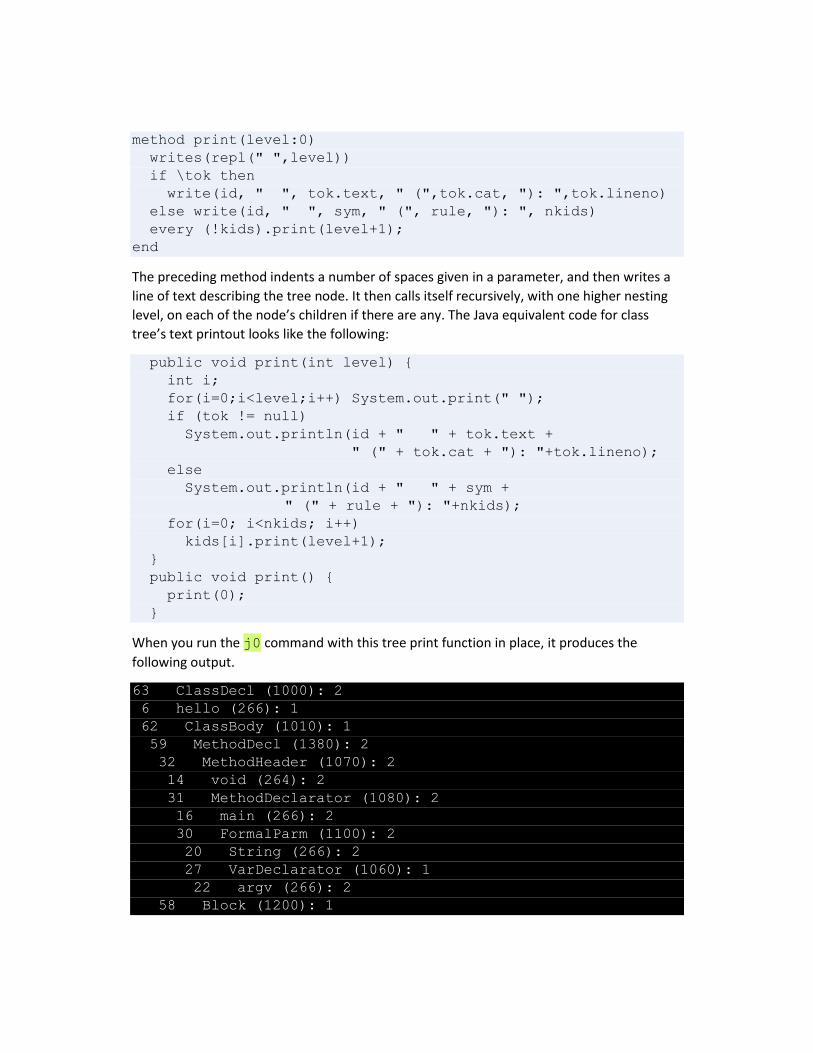
The preceding method indents a number of spaces given in a parameter, and then writes a

line of text describing the tree node. It then calls itself recursively, with one higher nesting

level, on each of the node’s children if there are any. The Java equivalent code for class

tree’s text printout looks like the following:

public void print(int level) {

int i;

for(i=0;i<level;i++) System.out.print(" ");

if (tok != null)

System.out.println(id + " " + tok.text +

" (" + tok.cat + "): "+tok.lineno);

else

System.out.println(id + " " + sym +

" (" + rule + "): "+nkids);

for(i=0; i<nkids; i++)

kids[i].print(level+1);

}

public void print() {

print(0);

}

When you run the j0 command with this tree print function in place, it produces the

following output.

63 ClassDecl (1000): 2

6 hello (266): 1

62 ClassBody (1010): 1

59 MethodDecl (1380): 2

32 MethodHeader (1070): 2

14 void (264): 2

31 MethodDeclarator (1080): 2

16 main (266): 2

30 FormalParm (1100): 2

20 String (266): 2

27 VarDeclarator (1060): 1

22 argv (266): 2

58 Block (1200): 1

53 MethodCall (1290): 2

46 QualifiedName (1040): 2

41 QualifiedName (1040): 2

36 System (266): 3

40 out (266): 3

45 println (266): 3

50 "hello, jzero!" (273): 3

no errors

Although the tree structure can be deciphered from studying this output, it is not exactly

transparent. The next section shows a graphic way to depict the tree.

Printing your tree using dot

The fun way to test your syntax tree is to print out the tree in a graphical form. As

mentioned in the System requirements section, a tool called dot will draw syntax trees for

us. Writing our tree in dot’s input format is done via another tree traversal in which each

node results in one or more lines of text output. To draw a graphic version of the tree,

change the j0.print() method to call the tree class print_graph() method. In

Unicon this is trivial.

method print(root)

root.print_graph(yyfilename || ".dot")

end

The equivalent code in Java must unpack the parserVal and cast the Object to a tree in order

to ask it to print itself.

public static void print(parserVal root) {

((tree)root.obj).print_graph(yyfilename + ".dot");

}

As was true for a text-only printout, trees print themselves recursively. The Unicon version

of class tree’s print_graph() method is shown in the following listing.

method print_graph(fw)

if type(filename) == "string" then {

fw := open(filename, "w") |

stop("can't open ", image(filename), " for writing")

write(fw, "digraph {")

print_graph(fw)

write(fw, "}")

close(fw)

}

else if \tok then print_leaf(fw)

else {

print_branch(fw)

every i := 1 to nkids do

if \kids[i] then {

write(fw, "N",id," -> N",kids[i].id,";")

kids[i].print_graph(fw)

} else {

write(fw, "N",id," -> N",id,"_",j,";")

write(fw, "N", id, "_", j,

" [label=\"Empty rule\"];")

j +:= 1

}

}

end

The Java implementation of print_graph() consists of two methods. The first is a public

method that takes a filename, opens that file for writing, and writes the whole graph to that

file.

void print_graph(String filename){

try {

PrintWriter pw = new PrintWriter(

new BufferedWriter(new FileWriter(filename)));

pw.printf("digraph {\n");

j = 0;

print_graph(pw);

pw.printf("}\n");

pw.close();

}

catch (java.io.IOException ioException) {

System.err.println("printgraph exception");

System.exit(1);

}

}

In Java function overloading allows a public and private parts of print_graph() to have

the same name. The two methods are distinguished by their different parameters. The

public print_graph() passes the file that it opens as a parameter to the following

method. This version of print_graph() prints a line or two about the current node, and

calls itself recursively on each child.

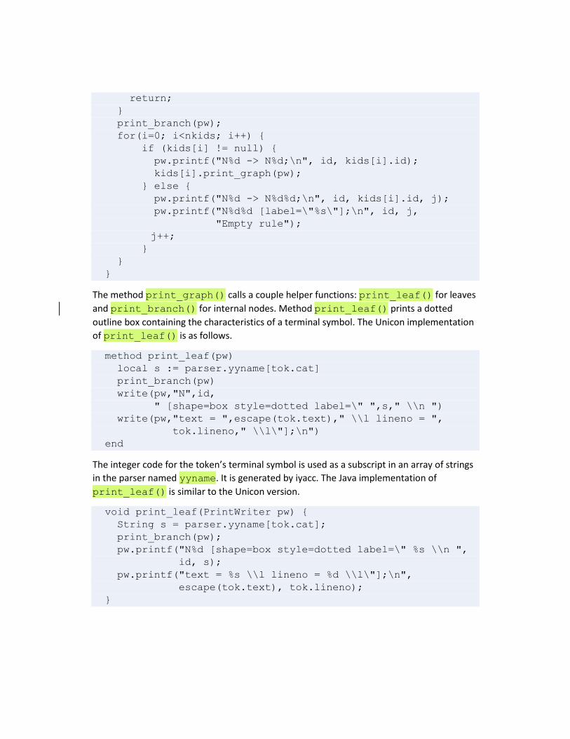
void print_graph(PrintWriter pw) {

int i;

if (tok != null) {

print_leaf(pw);

return;

}

print_branch(pw);

for(i=0; i<nkids; i++) {

if (kids[i] != null) {

pw.printf("N%d -> N%d;\n", id, kids[i].id);

kids[i].print_graph(pw);

} else {

pw.printf("N%d -> N%d%d;\n", id, kids[i].id, j);

pw.printf("N%d%d [label=\"%s\"];\n", id, j,

"Empty rule");

j++;

}

}

}

The method print_graph() calls a couple helper functions: print_leaf() for leaves

and print_branch() for internal nodes. Method print_leaf() prints a dotted

outline box containing the characteristics of a terminal symbol. The Unicon implementation

of print_leaf() is as follows.

method print_leaf(pw)

local s := parser.yyname[tok.cat]

print_branch(pw)

write(pw,"N",id,

" [shape=box style=dotted label=\" ",s," \\n ")

write(pw,"text = ",escape(tok.text)," \\l lineno = ",

tok.lineno," \\l\"];\n")

end

The integer code for the token’s terminal symbol is used as a subscript in an array of strings

in the parser named yyname. It is generated by iyacc. The Java implementation of

print_leaf() is similar to the Unicon version.

void print_leaf(PrintWriter pw) {

String s = parser.yyname[tok.cat];

print_branch(pw);

pw.printf("N%d [shape=box style=dotted label=\" %s \\n ",

id, s);

pw.printf("text = %s \\l lineno = %d \\l\"];\n",

escape(tok.text), tok.lineno);

}

Method print_branch() prints a solid box for internal nodes, including the name of the

non-terminal represented by that node. The Unicon implementation of print_branch()

is the following.

method print_branch(pw)

write(pw, "N",id," [shape=box label=\"",

pretty_print_name(),"\"];\n");

end

The Java implementation of print_branch() is similar to its Unicon counterpart.

void print_branch(PrintWriter pw) {

pw.printf("N%d [shape=box label=\"%s\"];\n",

id, pretty_print_name());

}

Method escape() adds escape characters when needed before double quotes so that dot

will print the double quote marks. The Unicon implementation of escape() consists of the

following.

method escape(s)

if s[1] == "\"" then

return "\\" || s[1:-1] || "\\\""

else return s

end

The Java implementation of escape() is as follows.

public String escape(String s) {

if (s.charAt(0) == '\"')

return "\\"+s.substring(0, s.length()-1)+"\\\"";

else return s;

}

Method pretty_print_name() prints out the best human-readable name for a given

node. For an internal node that is its string label, along with a serial number to distinguish

multiple occurrences of the same label. For a terminal symbol, it includes the lexeme

matched.

method pretty_print_name() {

if /tok then return sym || "#" || (rule%10)

else return escape(tok.text) || ":" || tok.cat

end

The Java implementation of pretty_print_name() looks similar to the preceding

code.

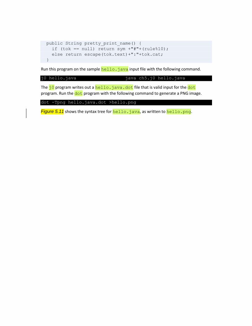
public String pretty_print_name() {

if (tok == null) return sym +"#"+(rule%10);

else return escape(tok.text)+":"+tok.cat;

}

Run this program on the sample hello.java input file with the following command.

j0 hello.java java ch5.j0 hello.java

The j0 program writes out a hello.java.dot file that is valid input for the dot

program. Run the dot program with the following command to generate a PNG image.

dot -Tpng hello.java.dot >hello.png

Figure 5.11 shows the syntax tree for hello.java, as written to hello.png.

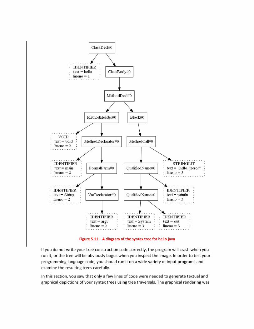
Figure 5.11 – A diagram of the syntax tree for hello.java

If you do not write your tree construction code correctly, the program will crash when you

run it, or the tree will be obviously bogus when you inspect the image. In order to test your

programming language code, you should run it on a wide variety of input programs and

examine the resulting trees carefully.

In this section, you saw that only a few lines of code were needed to generate textual and

graphical depictions of your syntax trees using tree traversals. The graphical rendering was

provided by an external tool called dot. Tree traversals are a simple but powerful

programming technique that will dominate the next several chapters of this book.

Summary

In this chapter, you learned the crucial technical skills and tools used to build a syntax tree

while the input program is being parsed. A syntax tree is the main data structure used to

represent the source code internally to a compiler or interpreter.

You learned how to develop a code that identifies what production rule was used to build

each internal node, so that we can tell what we are looking at later on. You learned how to

add tree node constructors for each rule in the scanner. You learned to connect tree leaves

from the scanner into the tree built in the parser. You learned to check your trees and

debug common tree construction problems.

You are done synthesizing the input source code to a data structure that you can use. Now it

is time to start analyzing the meaning of the program source code so you can determine

what computations it specifies. This is done by walking through the parse tree using tree

traversals to perform semantic analysis.

The next chapter will start us off on that journey by walking the tree to build symbol tables

that will enable you to track all the variables in the program and figure out where they were

declared.