Chapter 5: Marginal Costing - Ibrahim Sameer · Chapter 5: Marginal Costing 2016 ... problems will...
61
Chapter 5: Marginal Costing 2016 1 Ibrahim Sameer Bachelors of Business – Finance (CMA – Cyryx College) Cost & Management Accounting Bachelors of Business (Specialized in Finance) – Study Notes & Tutorial Questions Chapter 5: Marginal Costing
Transcript of Chapter 5: Marginal Costing - Ibrahim Sameer · Chapter 5: Marginal Costing 2016 ... problems will...

Chapter 5: Marginal Costing 2016
1 Ibrahim Sameer Bachelors of Business – Finance (CMA – Cyryx College)
Cost & Management Accounting
Bachelors of Business (Specialized in
Finance) – Study Notes & Tutorial
Questions
Chapter 5: Marginal Costing
Chapter 5: Marginal Costing 2016
2 Ibrahim Sameer Bachelors of Business – Finance (CMA – Cyryx College)
Introduction
Marginal costing is an alternative method of costing to absorption costing. In marginal costing,
only variable costs are charged as a cost of sale and a contribution is calculated (sales revenue
minus variable cost of sales). Closing inventories of work in progress or finished goods are
valued at marginal (variable) production cost. Fixed costs are treated as a period cost, and are
charged in full to the profit and loss account of the accounting period in which they are incurred.
The marginal production cost per unit of an item usually consists of the following.
Direct materials
Variable production overheads
Direct labour
Direct labour costs might be excluded from marginal costs when the work force is a given
number of employees on a fixed wage or salary. Even so, it is not uncommon for direct labour to
be treated as a variable cost, even when employees are paid a basic wage for a fixed working
week. If in doubt, you should treat direct labour as a variable cost unless given clear indications
to the contrary. Direct labour is often a step cost, with sufficiently short steps to make labour
costs act in a variable fashion.
The marginal cost of sales usually consists of the marginal cost of production adjusted for
inventory movements plus the variable selling costs, which would include items such as sales
commission, and possibly some variable distribution costs.
Chapter 5: Marginal Costing 2016
3 Ibrahim Sameer Bachelors of Business – Finance (CMA – Cyryx College)
The principles of Marginal Costing
The principles of marginal costing are as follows.
a) Period fixed costs are the same, for any volume of sales and production (provided that the
level of activity is within the 'relevant range'). Therefore, by selling an extra item of
product or service the following will happen.
(i) Revenue will increase by the sales value of the item sold.
(ii) Costs will increase by the variable cost per unit.
(iii) Profit will increase by the amount of contribution earned from the extra
item.
b) Similarly, if the volume of sales falls by one item, the profit will fall by the amount of
contribution earned from the item.
c) Profit measurement should therefore be based on an analysis of total contribution. Since
fixed costs relate to a period of time, and do not change with increases or decreases in
sales volume, it is misleading to charge units of sale with a share of fixed costs.
Absorption costing is therefore misleading, and it is more appropriate to deduct fixed
costs from total contribution for the period to derive a profit figure.
d) When a unit of product is made, the extra costs incurred in its manufacture are the
variable production costs. Fixed costs are unaffected, and no extra fixed costs are
incurred when output is increased. It is therefore argued that the valuation of closing
inventories should be at variable production cost (direct materials, direct labour, direct
expenses (if any) and variable production overhead) because these are the only costs
properly attributable to the product.
Break Even Point (BEP)
At this point there is neither profit nor loss; that is, the activity breaks even. Where the volume of
activity is below BEP, a loss will be incurred because total cost exceeds total sales revenue.
Where the business operates at a volume of activity above BEP, there will be a profit because
total sales revenue will exceed total cost. The further below BEP, the higher the loss: the further
above BEP, the higher the profit.

Chapter 5: Marginal Costing 2016
4 Ibrahim Sameer Bachelors of Business – Finance (CMA – Cyryx College)
Deducing BEPs by graphical means is a laborious business. Since the relationships in the graph
are all linear (that is, the lines are all straight), however, it is easy to calculate the BEP.
We know that at BEP (but not at any other point):
Total sales revenue = Total cost
If we call the number of units of output at BEP b, then
BEP (unit) = FC / Contribution per unit (SP – VC)
BEP ($) = FC + Target Profit / C.S Ratio
C/S Ratio = (sales revenue - cost of sales) / sales revenue x 100.

Chapter 5: Marginal Costing 2016
5 Ibrahim Sameer Bachelors of Business – Finance (CMA – Cyryx College)
If we look back at the break-even chart above, this formula seems logical. The total cost line
starts off at point F, higher than the starting point for the total sales revenues line (zero) by
amount F (the amount of the fixed cost). Because the sales revenue per unit is greater than the
variable cost per unit, the sales revenue line will gradually catch up with the total cost line. The
rate at which it will catch up is dependent on the relative steepness of the two lines. Bearing in
mind that the slopes of the two lines are the variable cost per unit and the selling price per unit,
the above equation for calculating b looks perfectly logical.
Though the BEP can be calculated quickly and simply without resorting to graphs, this does not
mean that the break-even chart is without value. The chart shows the relationship between cost,
volume and profit over a range of activity and in a form that can easily be understood by non-
financial managers. The break-even chart can therefore be a useful device for explaining this
relationship.
Contribution
Contribution is an important measure in marginal costing, and it is calculated as the difference
between sales value and marginal or variable cost of sales.
Contribution is of fundamental importance in marginal costing, and the term 'contribution' is
really short for 'contribution towards covering fixed overheads and making a profit'.
Chapter 5: Marginal Costing 2016
6 Ibrahim Sameer Bachelors of Business – Finance (CMA – Cyryx College)
Contribution margin ratio
The contribution margin ratio is the contribution from an activity expressed as a percentage of
the sales revenue, thus:
The ratio can provide an impression of the extent to which sales revenue is eaten away by
variable cost.
Profit or contribution information
The main advantage of contribution information (rather than profit information) is that it allows
an easy calculation of profit if sales increase or decrease from a certain level. By comparing total
contribution with fixed overheads, it is possible to determine whether profits or losses will be
made at certain sales levels. Profit information, on the other hand, does not lend itself to easy
manipulation but note how easy it was to calculate profits using contribution information in the
question entitled Marginal costing principles. Contribution information is more useful for
decision making than profit information.
Margin of safety
The margin of safety is the extent to which the planned volume of output or sales lies above the
BEP. The margin of safety can be used as a partial measure of risk.
Achieving a target profit
In the same way as we can derive the number of units of output necessary to break even, we can
calculate the volume of activity required to achieve a particular level of profit.
Chapter 5: Marginal Costing 2016
7 Ibrahim Sameer Bachelors of Business – Finance (CMA – Cyryx College)
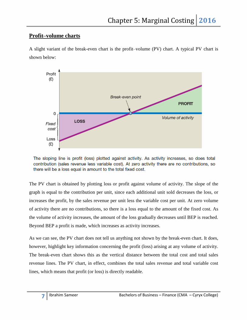
Profit–volume charts
A slight variant of the break-even chart is the profit–volume (PV) chart. A typical PV chart is
shown below:
The PV chart is obtained by plotting loss or profit against volume of activity. The slope of the
graph is equal to the contribution per unit, since each additional unit sold decreases the loss, or
increases the profit, by the sales revenue per unit less the variable cost per unit. At zero volume
of activity there are no contributions, so there is a loss equal to the amount of the fixed cost. As
the volume of activity increases, the amount of the loss gradually decreases until BEP is reached.
Beyond BEP a profit is made, which increases as activity increases.
As we can see, the PV chart does not tell us anything not shown by the break-even chart. It does,
however, highlight key information concerning the profit (loss) arising at any volume of activity.
The break-even chart shows this as the vertical distance between the total cost and total sales
revenue lines. The PV chart, in effect, combines the total sales revenue and total variable cost
lines, which means that profit (or loss) is directly readable.

Chapter 5: Marginal Costing 2016
8 Ibrahim Sameer Bachelors of Business – Finance (CMA – Cyryx College)
The economist’s view of the break-even chart
So far in this chapter we have treated all the relationships as linear – that is, all of the lines in the
graphs have been straight. This is typically the approach taken in management accounting,
though it may not be strictly valid.
Consider, for example, the variable cost line in the break-even chart; accountants would
normally treat this as being a straight line. Strictly, however, the line should probably not be
straight because at high levels of output economies of scale may be available to an extent not
available at lower levels. For example, a raw material (a typical variable cost) may be able to be
used more efficiently with higher volumes of activity. Similarly, buying large quantities of
material and services may enable the business to benefit from bulk discounts and so lower the
cost.
There is also a tendency for sales revenue per unit to reduce as volume is increased. To sell more
of a particular product or service, it will usually be necessary to lower the price per unit.
Economists recognise that, in real life, the relationships portrayed in the break-even chart are
usually non-linear. The typical economist’s view of the chart is shown in Figure below.

Chapter 5: Marginal Costing 2016
9 Ibrahim Sameer Bachelors of Business – Finance (CMA – Cyryx College)
Note, above figure, that the total variable cost line starts to rise quite steeply with volume but,
around point A, economies of scale start to take effect. With further increases in volume, total
variable cost does not rise as steeply because the variable cost for each additional unit of output
is lowered. These economies of scale continue to have a benign effect on cost until a point is
reached where the business is operating towards the end of its efficient range. Beyond this range,
problems will emerge that adversely affect variable cost. For example, the business may be
unable to find cheap supplies of the variable-cost elements or may suffer production difficulties,
such as machine breakdowns. As a result, the total variable cost line starts to rise more steeply.
At low levels of output, sales may be made at a relatively high price per unit. To increase sales
output beyond point B, however, it may be necessary to lower the average sales price per unit.
This will mean that the total revenue line will not rise as steeply, and may even curve
downwards.
Note how this ‘curvilinear’ representation of the break-even chart can easily lead to the existence
of two break-even points.
Chapter 5: Marginal Costing 2016
10 Ibrahim Sameer Bachelors of Business – Finance (CMA – Cyryx College)
Accountants justify their approach to this topic by the fact that, though the lines may not, in
practice, be perfectly straight, this defect is probably not worth taking into account in most cases.
This is partly because all of the information used in the analysis is based on estimates of the
future. As this will inevitably be flawed, it seems pointless to be pedantic about the minor
approximation of treating the total cost and total revenue lines as straight when strictly this is not
so. Only where significant economies or diseconomies of scale are involved should the non-
linearity of the variable cost be taken into account. Also, for most businesses, the range of
possible volumes of activity at which they are capable of operating (the relevant range) is pretty
narrow. Over very short distances, it may be perfectly reasonable to treat a curved line as being
straight.
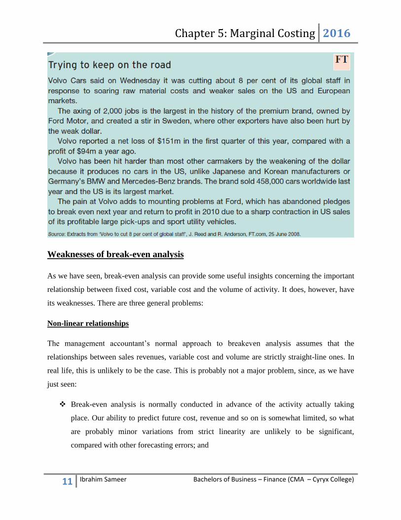
Failing to break even
Where a business fails to reach its BEP, steps must be taken to remedy the problem: there must
be an increase in sales revenue or a reduction in cost, or both of these. Below case discusses how
Ford’s subsidiary Volvo is struggling to reach its BEP. Ford has recently disposed of its three
UK luxury brands (Aston Martin, Jaguar and Land Rover) and is thought to be considering the
possibility of selling off Volvo as well.
Chapter 5: Marginal Costing 2016
11 Ibrahim Sameer Bachelors of Business – Finance (CMA – Cyryx College)
Weaknesses of break-even analysis
As we have seen, break-even analysis can provide some useful insights concerning the important
relationship between fixed cost, variable cost and the volume of activity. It does, however, have
its weaknesses. There are three general problems:
Non-linear relationships
The management accountant’s normal approach to breakeven analysis assumes that the
relationships between sales revenues, variable cost and volume are strictly straight-line ones. In
real life, this is unlikely to be the case. This is probably not a major problem, since, as we have
just seen:
Break-even analysis is normally conducted in advance of the activity actually taking
place. Our ability to predict future cost, revenue and so on is somewhat limited, so what
are probably minor variations from strict linearity are unlikely to be significant,
compared with other forecasting errors; and
Chapter 5: Marginal Costing 2016
12 Ibrahim Sameer Bachelors of Business – Finance (CMA – Cyryx College)
Most businesses operate within a narrow range of volume of activity; over short ranges,
curved lines tend to be relatively straight.
Stepped fixed cost
Most types of fixed cost are not fixed over all volumes of activity. They tend to be ‘stepped’
fixed cost. This means that, in practice, great care must be taken in making assumptions about
fixed cost. The problem is heightened because most activities will probably involve various types
of fixed cost (for example rent, supervisory salaries, administration cost), all of which are likely
to have steps at different points.
Multi-product businesses
Most businesses do not offer just one product or service. This is a problem for break-even
analysis since it raises the question of the effect of additional sales of one product or service on
sales of another of the business’s products or services. There is also the problem of identifying
the fixed cost of one particular activity. Fixed cost tends to relate to more than one activity – for
example, two activities may be carried out in the same rented premises. There are ways of
dividing the fixed cost between activities, but these tend to be arbitrary, which calls into question
the value of the break-even analysis and any conclusions reached.

Chapter 5: Marginal Costing 2016
13 Ibrahim Sameer Bachelors of Business – Finance (CMA – Cyryx College)
Marginal costing and absorption costing and the calculation of Profit
In marginal costing, fixed production costs are treated as period costs and are written off as they
are incurred. In absorption costing, fixed production costs are absorbed into the cost of units and
are carried forward in inventory to be charged against sales for the next period. Inventory values
using absorption costing are therefore greater than those calculated using marginal costing.
Marginal costing as a cost accounting system is significantly different from absorption costing. It
is an alternative method of accounting for costs and profit, which rejects the principles of
absorbing fixed overheads into unit costs.
Note
The share of fixed overheads included in cost of sales are from the previous period (in opening
inventory values). Some of the fixed overheads from the current period will be excluded by
being carried forward in closing inventory values.
In marginal costing, it is necessary to identify the following.
Variable costs
Fixed costs
Contribution
In absorption costing (sometimes known as full costing), it is not necessary to distinguish
variable costs from fixed costs.
Chapter 5: Marginal Costing 2016
14 Ibrahim Sameer Bachelors of Business – Finance (CMA – Cyryx College)
Reconciling profits
Reported profit figures using marginal costing or absorption costing will differ if there is any
change in the level of inventories in the period. If production is equal to sales, there will be no
difference in calculated profits using the costing methods.
If inventory levels increase between the beginning and end of a period, absorption costing will
report the higher profit. This is because some of the fixed production overhead incurred during
the period will be carried forward in closing inventory (which reduces cost of sales) to be set
against sales revenue in the following period instead of being written off in full against profit in
the period concerned.
If inventory levels decrease, absorption costing will report the lower profit because as well as the
fixed overhead incurred, fixed production overhead which had been carried forward in opening
inventory is released and is also included in cost of sales.
Reconciling profits – a shortcut
A quick way to establish the difference in profits without going through the whole process of
drawing up the income statements is as follows.
Difference in profits = change in inventory level x overhead absorption rate per unit
If inventory levels have gone up (that is, closing inventory > opening inventory) then absorption
costing profit will be greater than marginal costing profit.
If inventory levels have gone down (that is, closing inventory < opening inventory) then
absorption costing profit will be less than marginal costing profit.
Marginal costing versus absorption costing
Absorption costing is most often used for routine profit reporting and must be used for financial
accounting purposes. Marginal costing provides better management information for planning and
decision making. There are a number of arguments both for and against each of the costing
systems.
Chapter 5: Marginal Costing 2016
15 Ibrahim Sameer Bachelors of Business – Finance (CMA – Cyryx College)
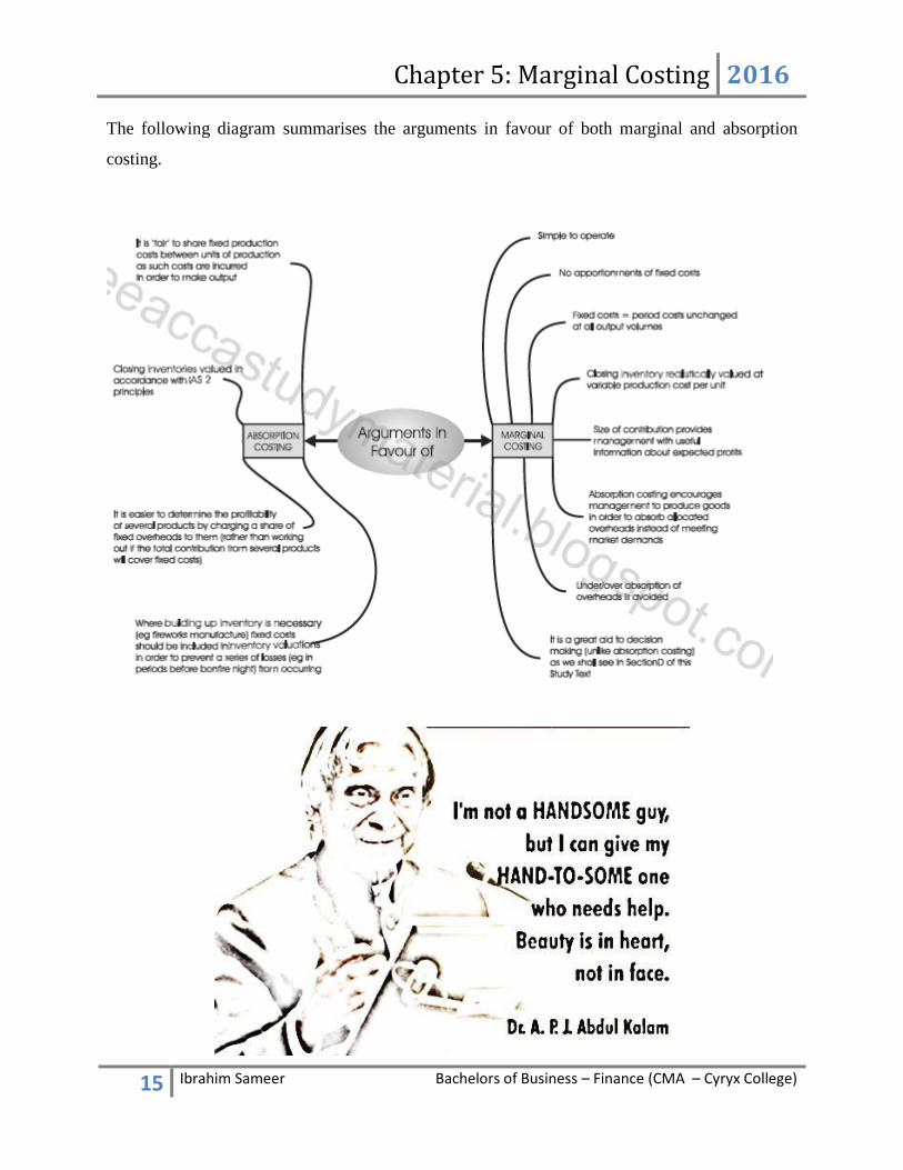
The following diagram summarises the arguments in favour of both marginal and absorption
costing.
Chapter 5: Marginal Costing 2016
16 Ibrahim Sameer Bachelors of Business – Finance (CMA – Cyryx College)
Practice Questions
Question 1
Question 2
Question 3
In practice, relationships between costs, revenues and volumes of activity are not necessarily
straight-line ones. Can you think of at least three reasons, with examples, why this may be the
case?
Chapter 5: Marginal Costing 2016
17 Ibrahim Sameer Bachelors of Business – Finance (CMA – Cyryx College)
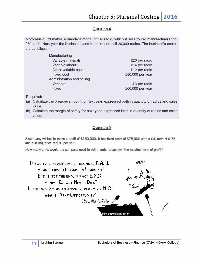
Question 4
Question 5
Chapter 5: Marginal Costing 2016
18 Ibrahim Sameer Bachelors of Business – Finance (CMA – Cyryx College)
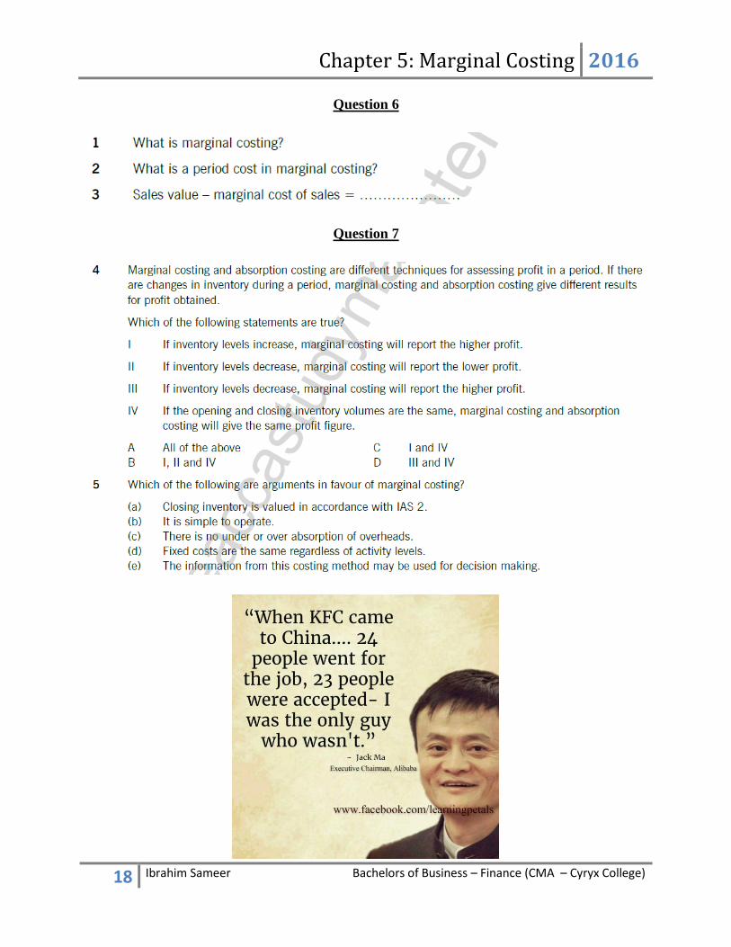
Question 6
Question 7
Chapter 5: Marginal Costing 2016
19 Ibrahim Sameer Bachelors of Business – Finance (CMA – Cyryx College)
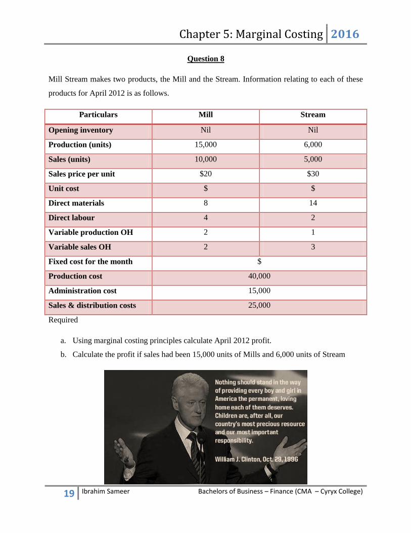
Question 8
Mill Stream makes two products, the Mill and the Stream. Information relating to each of these
products for April 2012 is as follows.
Particulars Mill Stream
Opening inventory Nil Nil
Production (units) 15,000 6,000
Sales (units) 10,000 5,000
Sales price per unit $20 $30
Unit cost $ $
Direct materials 8 14
Direct labour 4 2
Variable production OH 2 1
Variable sales OH 2 3
Fixed cost for the month $
Production cost 40,000
Administration cost 15,000
Sales & distribution costs 25,000
Required
a. Using marginal costing principles calculate April 2012 profit.
b. Calculate the profit if sales had been 15,000 units of Mills and 6,000 units of Stream

Chapter 5: Marginal Costing 2016
20 Ibrahim Sameer Bachelors of Business – Finance (CMA – Cyryx College)
Question 9
Big Woof Co manufactures a single product, the Bark, details of which are as follows.
Per unit $
Selling price 180,000
Direct materials 40,000
Direct labour 16,000
Variable OH 10,000
Annual fixed production OH are budgeted to be $1,600,000 and Big Woof expects to produce
1,280,000 units of the Bark each year. OH are absorbed on a per unit basis. Actual OH are
$1,600,000 for the year.
Budgeted fixed selling costs are $320,000 per quarter.
Actual sales and production units for the first quarter of 2012 are given below.
January – March
Sales 240,000
Production 280,000
There is no opening inventory at the beginning of January.
Prepare income statement for the quarter, using
a. Marginal costing
b. Absorption costing
Question 10
When opening inventories were 8,500 litres and closing inventories 6,750 litres, a firm has a
profit of $62,100 using marginal costing.
Assuming that the fixed OH absorption rate was $3 per litre, what would be the profit using
absorption costing?
Chapter 5: Marginal Costing 2016
21 Ibrahim Sameer Bachelors of Business – Finance (CMA – Cyryx College)
Question 11
Last month a manufacturing company’s profit was $2,000, calculated using absorption costing
principles. If marginal costing principles has been used, a loss of $3,000 would have occurred.
The company’s fixed production cost is $2 per unit. Sales last month were 10,000 units.
What was last month’s production (in units)?
Question 12
In a period where opening inventory were 16,000 units and closing inventories were 21,000
units, a firm had a profit of $140,000 using absorption costing. If the fixed OAR was $8.50 per
unit. Calculate profit using marginal costing method.
Question 13
A company had opening inventory of 49,300 units and closing inventory of 44,900 units. Profit
based on marginal costing were $320,350 and on absorption costing were $298,650. What is the
fixed OAR per unit?

Chapter 5: Marginal Costing 2016
22 Ibrahim Sameer Bachelors of Business – Finance (CMA – Cyryx College)
Question 14
A company produces and sells a single product whose variable cost is $7 per unit.
Fixed costs have been absorbed over the normal level of activity of 250,000 units and have been
calculated as $2.50 per unit.
The current selling price is $11 per unit.
How much profit is made under marginal costing if the company sells 300,000 units?
Question 15
HMF Co produces a single product. The budgeted fixed production OH for the period are
$550,000. The budgeted output for the period is 3,500 units. Opening inventory at the start of the
period consisted of 950 units and closing inventory at the end of the period consisted of 350
units. If absorption costing principles were applied, calculate the profit for the period compared
to the marginal costing profit.
Question 16
Chapter 5: Marginal Costing 2016
23 Ibrahim Sameer Bachelors of Business – Finance (CMA – Cyryx College)
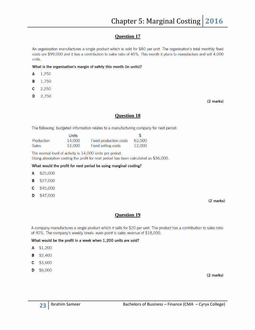
Question 17
Question 18
Question 19
Chapter 5: Marginal Costing 2016
24 Ibrahim Sameer Bachelors of Business – Finance (CMA – Cyryx College)
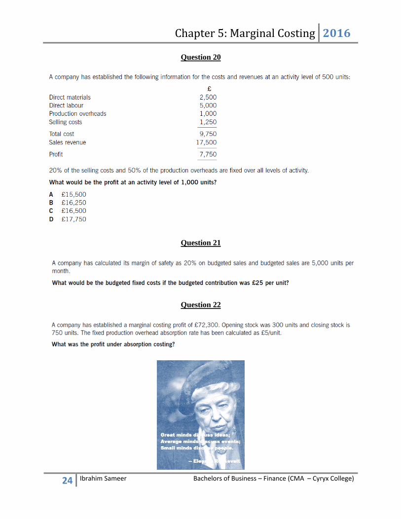
Question 20
Question 21
Question 22

Chapter 5: Marginal Costing 2016
25 Ibrahim Sameer Bachelors of Business – Finance (CMA – Cyryx College)
Question 23
Question 24
Question 25
Question 26
Chapter 5: Marginal Costing 2016
26 Ibrahim Sameer Bachelors of Business – Finance (CMA – Cyryx College)
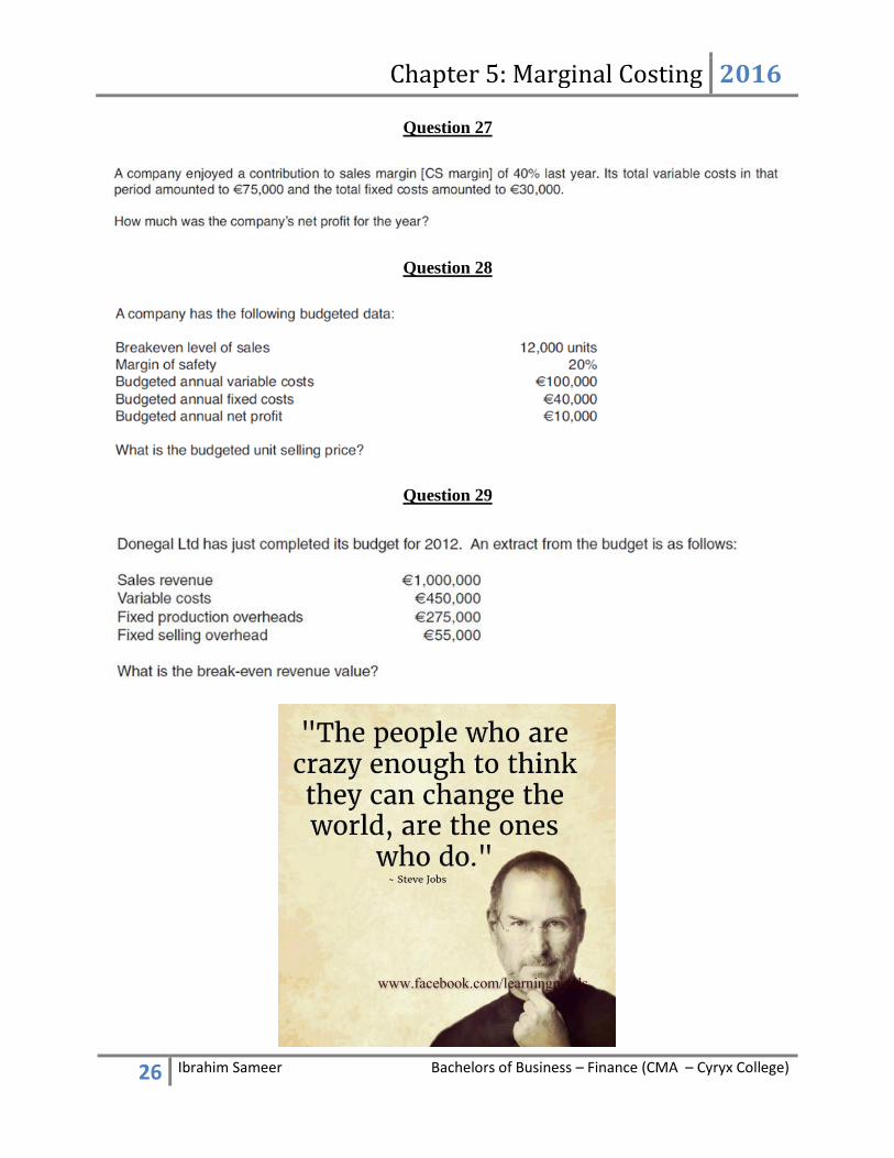
Question 27
Question 28
Question 29
Chapter 5: Marginal Costing 2016
27 Ibrahim Sameer Bachelors of Business – Finance (CMA – Cyryx College)
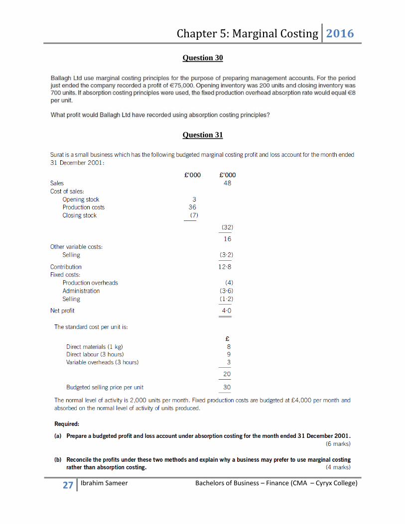
Question 30
Question 31

Chapter 5: Marginal Costing 2016
28 Ibrahim Sameer Bachelors of Business – Finance (CMA – Cyryx College)
Question 32
Chapter 5: Marginal Costing 2016
29 Ibrahim Sameer Bachelors of Business – Finance (CMA – Cyryx College)
Question 33
Chapter 5: Marginal Costing 2016
30 Ibrahim Sameer Bachelors of Business – Finance (CMA – Cyryx College)
Question 34

Chapter 5: Marginal Costing 2016
31 Ibrahim Sameer Bachelors of Business – Finance (CMA – Cyryx College)
Question 35

Chapter 5: Marginal Costing 2016
32 Ibrahim Sameer Bachelors of Business – Finance (CMA – Cyryx College)
Question 36
Question 37
Question 38
Chapter 5: Marginal Costing 2016
33 Ibrahim Sameer Bachelors of Business – Finance (CMA – Cyryx College)
Question 39
Question 40
Question 41
Question 42
Chapter 5: Marginal Costing 2016
34 Ibrahim Sameer Bachelors of Business – Finance (CMA – Cyryx College)
Question 43
Question 44
Question 45

Chapter 5: Marginal Costing 2016
35 Ibrahim Sameer Bachelors of Business – Finance (CMA – Cyryx College)
Question 46
Question 47
Question 48
Chapter 5: Marginal Costing 2016
36 Ibrahim Sameer Bachelors of Business – Finance (CMA – Cyryx College)
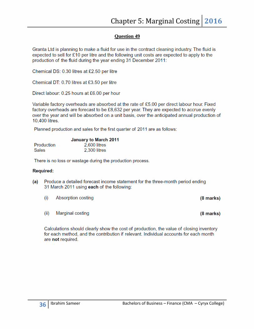
Question 49
Chapter 5: Marginal Costing 2016
37 Ibrahim Sameer Bachelors of Business – Finance (CMA – Cyryx College)
Chapter 5: Marginal Costing 2016
38 Ibrahim Sameer Bachelors of Business – Finance (CMA – Cyryx College)
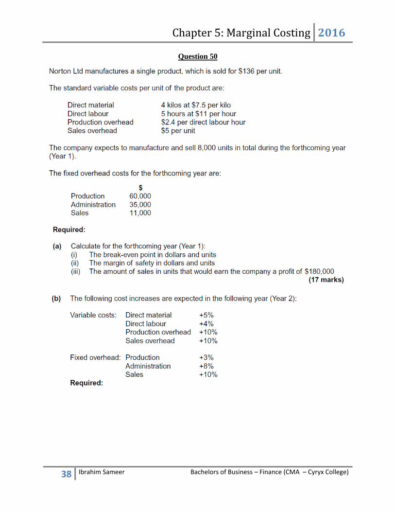
Question 50
Chapter 5: Marginal Costing 2016
39 Ibrahim Sameer Bachelors of Business – Finance (CMA – Cyryx College)

Chapter 5: Marginal Costing 2016
40 Ibrahim Sameer Bachelors of Business – Finance (CMA – Cyryx College)
Question 51

Chapter 5: Marginal Costing 2016
41 Ibrahim Sameer Bachelors of Business – Finance (CMA – Cyryx College)
Question 52

Chapter 5: Marginal Costing 2016
42 Ibrahim Sameer Bachelors of Business – Finance (CMA – Cyryx College)
Question 53
Chapter 5: Marginal Costing 2016
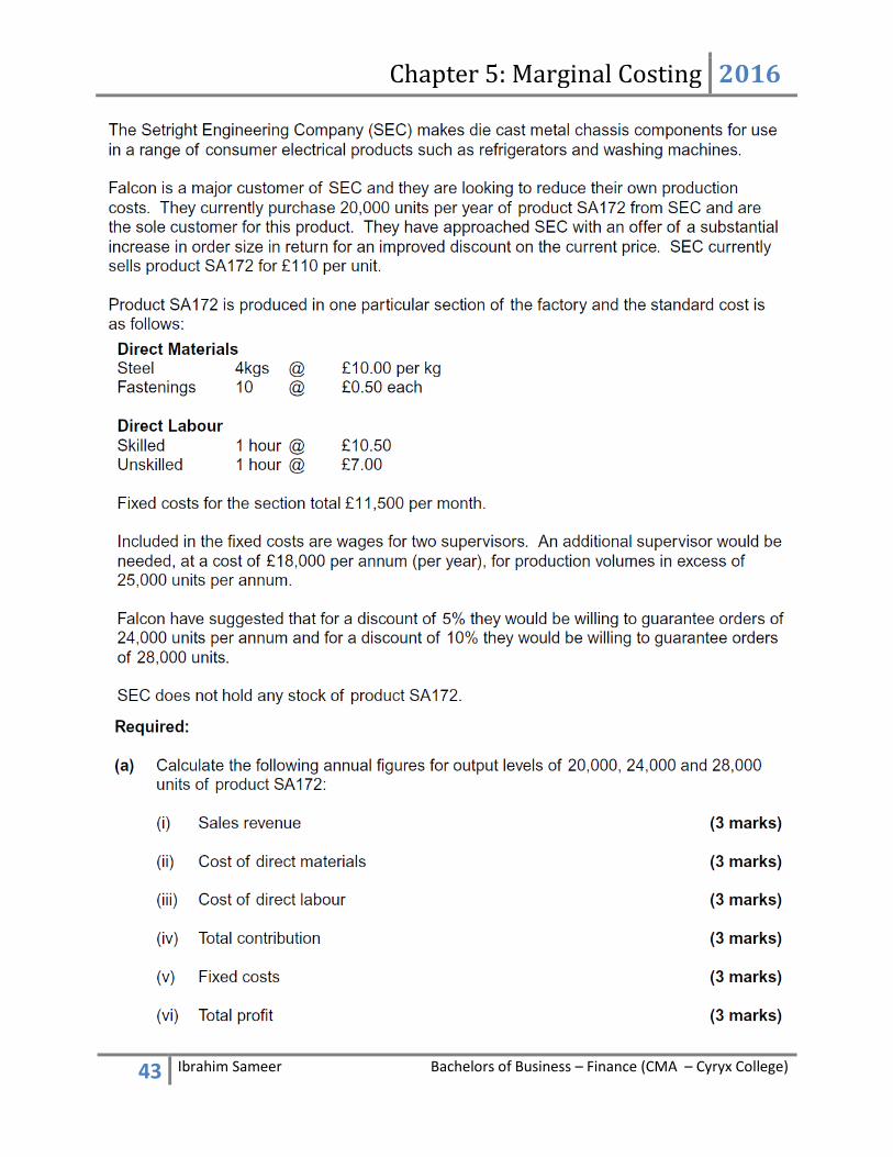
43 Ibrahim Sameer Bachelors of Business – Finance (CMA – Cyryx College)
Chapter 5: Marginal Costing 2016
44 Ibrahim Sameer Bachelors of Business – Finance (CMA – Cyryx College)
Chapter 5: Marginal Costing 2016
45 Ibrahim Sameer Bachelors of Business – Finance (CMA – Cyryx College)
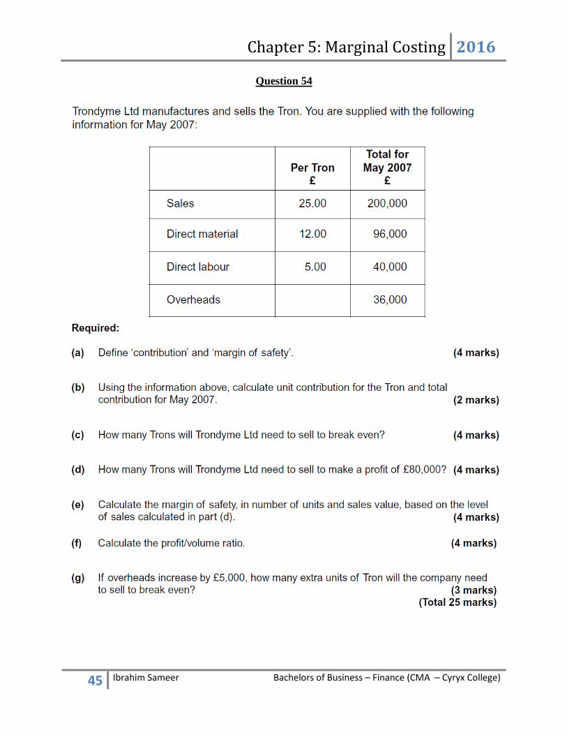
Question 54

Chapter 5: Marginal Costing 2016
46 Ibrahim Sameer Bachelors of Business – Finance (CMA – Cyryx College)
Question 55

Chapter 5: Marginal Costing 2016
47 Ibrahim Sameer Bachelors of Business – Finance (CMA – Cyryx College)
Question 56
Chapter 5: Marginal Costing 2016
48 Ibrahim Sameer Bachelors of Business – Finance (CMA – Cyryx College)
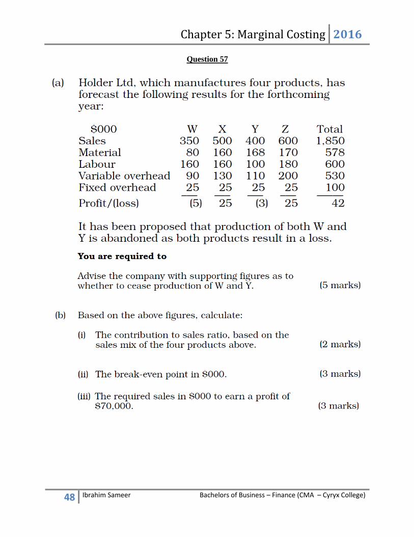
Question 57
Chapter 5: Marginal Costing 2016
49 Ibrahim Sameer Bachelors of Business – Finance (CMA – Cyryx College)
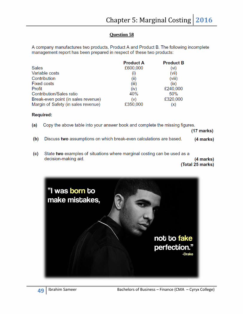
Question 58

Chapter 5: Marginal Costing 2016
50 Ibrahim Sameer Bachelors of Business – Finance (CMA – Cyryx College)
Question 59
Chapter 5: Marginal Costing 2016
51 Ibrahim Sameer Bachelors of Business – Finance (CMA – Cyryx College)
Chapter 5: Marginal Costing 2016
52 Ibrahim Sameer Bachelors of Business – Finance (CMA – Cyryx College)
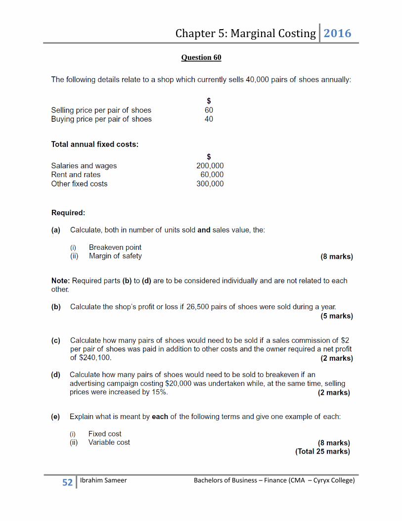
Question 60

Chapter 5: Marginal Costing 2016
53 Ibrahim Sameer Bachelors of Business – Finance (CMA – Cyryx College)
Question 61
Question 62
Question 63
Question 64

Chapter 5: Marginal Costing 2016
54 Ibrahim Sameer Bachelors of Business – Finance (CMA – Cyryx College)
Question 65
Question 66
Question 67
Question 68
Chapter 5: Marginal Costing 2016
55 Ibrahim Sameer Bachelors of Business – Finance (CMA – Cyryx College)
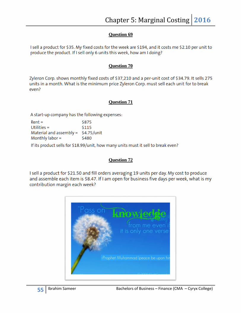
Question 69
Question 70
Question 71
Question 72
Chapter 5: Marginal Costing 2016
56 Ibrahim Sameer Bachelors of Business – Finance (CMA – Cyryx College)
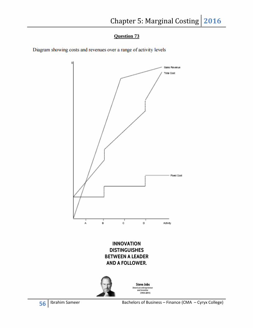
Question 73

Chapter 5: Marginal Costing 2016
57 Ibrahim Sameer Bachelors of Business – Finance (CMA – Cyryx College)
Question 74

Chapter 5: Marginal Costing 2016
58 Ibrahim Sameer Bachelors of Business – Finance (CMA – Cyryx College)
Question 75
Question 76

Chapter 5: Marginal Costing 2016
59 Ibrahim Sameer Bachelors of Business – Finance (CMA – Cyryx College)
Question 77
Question 78

Chapter 5: Marginal Costing 2016
60 Ibrahim Sameer Bachelors of Business – Finance (CMA – Cyryx College)
Question 79
Chapter 5: Marginal Costing 2016
61 Ibrahim Sameer Bachelors of Business – Finance (CMA – Cyryx College)
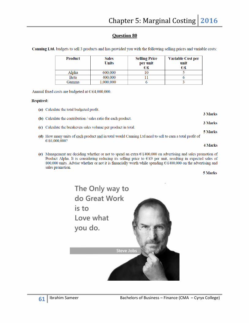
Question 80